SISSA 54/2009/EP

Gravity duals of 2d supersymmetric gauge theories

Daniel Areán ^†, Eduardo Conde ^∗, and Alfonso V. Ramallo^∗

^∗ Departamento de Física de Partículas, Universidade de Santiago de Compostela
and
Instituto Galego de Física de Altas Enerxías (IGFAE)
E-15782, Santiago de Compostela, Spain
^† SISSA and INFN-Sezione di Trieste
Via Beirut 2; I-34014
Trieste, Italy

Abstract

We find new supergravity solutions generated by D5-branes wrapping a four-cycle and preserving four and two supersymmetries. We first consider the configuration in which the fivebranes wrap a four-cycle in a Calabi-Yau threefold, which preserves four supersymmetries and is a gravity dual to the Coulomb branch of two-dimensional gauge theories with ${\cal N}=(2,2)$ supersymmetry. We also study the case of fivebranes wrapping a co-associative four-cycle in a manifold of $G_{2}$-holonomy, which provides a gravity dual of ${\cal N}=(1,1)$ supersymmetric Yang-Mills theory in two dimensions. We also discuss the addition of unquenched fundamental matter fields to these backgrounds and find the corresponding gravity solutions with flavor brane sources.

1 Introduction

The construction of supergravity solutions with a reduced number of supersymmetries has been one of the main research directions in the continuous effort to make the gauge/gravity correspondence [1, 2] closer to more realistic theories of Nature.

An approach that has been very fruitful in recent years is the analysis of supergravity solutions that correspond to branes wrapping supersymmetric cycles inside a non-compact manifold of special holonomy [3]. These solutions have various background fluxes turned on and provide us with gravity duals of supersymmetric Yang-Mills (SYM) theories living on the unwrapped part of the brane. As notable examples of these backgrounds, let us mention the one obtained in [4], and interpreted in [5] as the gravity dual of ${\cal N}=1$ SYM theory in four dimensions. This background corresponds to fivebranes wrapping a two-cycle. Similarly, in refs. [6, 7] the supergravity dual of ${\cal N}=2$ SYM in $d=4$ was found, also from fivebranes wrapping a two-cycle. Moreover, by wrapping a fivebrane in a three-cycle we can generate the supergravity dual of SYM in three space-time dimensions with different amounts of supersymmetry. This program was carried out in refs. [8, 9, 10] for ${\cal N}=1$ 3d SYM theory, whereas the background dual to ${\cal N}=2$ SYM in $d=3$ was found in refs. [11, 12].

In this paper we will continue with this line of research by considering D5-branes wrapping four-cycles and preserving different amounts of supersymmetry, whose corresponding dual field theories are two-dimensional. We will consider first the case in which the branes wrap a four-cycle of a Calabi-Yau threefold and four supersymmetries are preserved. The supersymmetry of the corresponding two-dimensional dual field theory is ${\cal N}=(2,2)$. We will then analyze the configuration in which the special holonomy manifold has $G_{2}$ holonomy and the number of supersymmetries preserved is two, which leads to ${\cal N}=(1,1)$ supersymmetry in the dual field theory. We will argue that these backgrounds are the gravitational duals of a slice of the Coulomb branch of the corresponding gauge theories. Moreover, we will also analyze the addition of unquenched flavor to both setups.

When dealing with backgrounds generated by wrapped branes a useful tool is the use of an appropriate lower-dimensional gauged supergravity [3], in which the brane worldvolume is a domain wall object of codimension one in the lower dimensional space-time. Thus, to obtain fivebrane solutions the appropriate gauged supergravity must be seven-dimensional. Moreover, in order to find supersymmetric solutions of wrapped branes in this approach one has to identify the spin connection along the wrapped cycle with some particular gauge fields of the gauged supergravity. This is an implementation of the so-called “topological twist”, needed to realize supersymmetry in the D-brane worldvolume [13]. In this paper we will use $SO(4)$ gauged supergravity [14, 15], which turns out to be the one needed to accommodate the twistings required for our solutions.

Once the metric and gauge fields in seven dimensions are known, one can obtain the metric and RR three-form of the ten-dimensional background by using the corresponding uplifting formulae [16]. In general, the results obtained by this procedure for our systems are rather complicated and the corresponding expressions for the metric and three-form that we will get involve coordinates that are non-trivially fibered. However, there is a change of variables, generalizing the one in [17] for the gravity dual of ${\cal N}=2$, $d=4$ SYM, which makes the results more transparent and neat. In this new system of coordinates the directions parallel and transverse to the special holonomy manifold are clearly distinguished. The price that one has to pay for this extra clarity is that all functions of the ansatz depend on two non-compact variables. Despite this fact, we will formulate our setup in terms of the ten-dimensional variables and we will impose the preservation of supersymmetry directly in ten-dimensions. This condition will lead us to a system of first-order BPS equations in partial derivatives for the functions entering our ansatz. After performing the corresponding uplifting and change of variables, the gauged supergravity approach provides a particular non-trivial analytic solution for this system of BPS equations. Other analytic solutions of the BPS system, not derived from gauged supergravity, will also be obtained.

The addition of matter degrees of freedom in the fundamental representation of the gauge group is another generalization of the gauge/gravity correspondence of obvious interest. The (by now) standard method to add this new matter sector in the correspondence consists of the inclusion of flavor branes, which should extend along all the gauge theory directions and wrap a non-compact cycle in the special holonomy manifold in order to make its worldvolume symmetry a global symmetry from the gauge theory point of view [18]. If the number of flavors, $N_{f}$, is small compared with the number of colors $N_{c}$, the flavor branes can be treated as probes in the background created by the color branes. On the contrary, when the number of flavors is of the order of the number of colors ($N_{f}\sim N_{c}$) one necessarily has to include the backreaction of the flavor branes on the geometry. In this case the flavor branes should be considered as dynamical sources of the different supergravity fields.

In this paper we will try to add flavor to the two types of wrapped fivebrane backgrounds studied. We will include the backreaction following the approach of ref. [19], in which the localized brane sources are substituted by a continuous distribution (see also [20]). This approach has been successfully applied in several brane setups ([21]-[36]). Here, we will be able to find a satisfactory implementation of this flavoring procedure for our background with four supersymmetries. However, in the case of the background dual to ${\cal N}=(1,1)$ supersymmetric field theory we will face new difficulties to determine the appropriate deformation introduced by the flavor branes. Nevertheless, we will be able to find the general structure of this deformation and we will find the corresponding backreacted background in terms of an unknown function satisfying a set of conditions.

The rest of this paper is organized as follows. In section 2 we will present our brane setup for the case in which four supersymmetries are preserved and we will specify our ansatz for the ten-dimensional metric and RR three-form. We will obtain a system of BPS differential equations and we will study the solution obtained from seven-dimensional gauged supergravity. The steps followed to find this solution will be detailed in appendix A. We will end section 2 by presenting the flavored version of the dual to the ${\cal N}=(2,2)$ theory. In section 3 we analyze the background preserving two supersymmetries. After an initial motivation, we will formulate our ansatz and we will find the corresponding system of BPS equations. Again, gauged supergravity provides a non-trivial solution of these equations, which will be explored from the ten-dimensional point of view in section 3, leaving the details of the gauged supergravity analysis to appendix A. We will finish section 3 by presenting our approach to add flavor to the ${\cal N}=(1,1)$ gravity dual. Section 4 contains our conclusions and summarizes our main results.

The paper ends with three appendices containing technical details which can be skipped in a first reading. In appendix A the gauged supergravity approach is presented, while in appendix B we study additional solutions of the ten-dimensional unflavored BPS systems. Finally, in appendix C we check that the second order equations of motion for the gravity plus brane sources systems are satisfied by any solution of the first-order BPS equations.

2 The dual of the ${\cal N}=(2,2)$ theory

The first case we will study corresponds to a background of type IIB supergravity generated by a stack of $N_{c}$ D5-branes wrapping a four-cycle ${\cal C}_{4}$ of a Calabi-Yau (CY) cone of complex dimension three. To simplify matters we will restrict to the case in which ${\cal C}_{4}$ is the product ${\cal C}_{2}\times{\cal C}_{2}$ of two two-cycles ${\cal C}_{2}$. The corresponding brane array is:

			$\overbrace{\phantom{\qquad\qquad\qquad\qquad\qquad}}^{\text{CY}_{3}}$
	$\mathbb{R}^{1,1}$		$S^{2}$		$S^{2}$		$N_{2}$		$\mathbb{R}^{2}$
$N_{c}$ D$5$	$-$	$-$	$\bigcirc$	$\bigcirc$	$\bigcirc$	$\bigcirc$	$\cdot$	$\cdot$	$\cdot$	$\cdot$

where the $S^{2}$’s represent the directions of the two-cycles ${\cal C}_{2}$ and $N_{2}$ are the directions of the normal bundle to ${\cal C}_{4}$. Notice that the symbols “$-$” and “$\cdot$” represent unwrapped worldvolume directions and directions transverse to the brane respectively, whereas a circle denotes a wrapped worldvolume direction.

In order to write a concrete ansatz for the metric of this array, let us parametrize the two two-cycles by two angles $(\theta_{i},\phi_{i})$, with $0\leq\theta_{i}\leq\pi$ and $0\leq\phi_{i}<2\pi$ ($i=1,2$), and let $\sigma$ represent the radial coordinate of the CY cone. We will also parametrize the transverse $\mathbb{R}^{2}$ space by another radial coordinate $\rho$, as well as by another angle $\chi$ ($0\leq\chi<2\pi$). Given these coordinates, the ansatz we will adopt for the string frame metric is:

$$ds^{2}\,=\,e^{\Phi}\,\,\Big{[}\,dx_{1,1}^{2}\,+\,{z\over m^{2}}\,\,\Big{(}\,d\theta_{1}^{2}\,+\,\sin^{2}\theta_{1}\,d\phi_{1}^{2}\,+\,d\theta_{2}^{2}\,+\,\sin^{2}\theta_{2}\,d\phi_{2}^{2}\,\Big{)}\,\Big{]}\,+\,$$

$$\,\,\,\,\,+\,{e^{-\Phi}\over m^{2}z^{2}}\,\Big{[}\,d\sigma^{2}\,+\,\sigma^{2}\,\Big{(}\,d\psi+\cos\theta_{1}d\phi_{1}\,+\,\cos\theta_{2}d\phi_{2}\,\Big{)}^{2}\,\Big{]}+{e^{-\Phi}\over m^{2}}\,\Big{(}\,d\rho^{2}\,+\,\rho^{2}\,d\chi^{2}\,\Big{)}\,\,,\qquad\qquad$$ (2.1)

where $m$ is a constant with units of mass which, for convenience, we will take as:

$$m^{2}\,=\,{1\over g_{s}\alpha^{\prime}N_{c}}\,\,,$$ (2.2)

with $g_{s}$ and $\alpha^{\prime}$ being respectively the string coupling constant and the Regge slope of superstring theory. Notice that $\psi$ ($0\leq\psi<2\pi$) is an angular coordinate along $N_{2}$, which is fibered over ${\cal C}_{2}\times{\cal C}_{2}$ as in the metric of the conifold. In (2.1) $dx_{1,1}^{2}$ is the Minkowski metric in 1+1 dimensions, $\Phi$ is the dilaton of the type IIB theory and $z$ is a function that controls the size of the cycle. The dilaton $\Phi$ and the function $z$ should be considered as functions of the two radial variables $(\rho,\sigma)$:

$$\Phi\,=\,\Phi(\rho,\sigma)\,\,,\qquad\qquad z\,=\,z(\rho,\sigma)\,\,.$$ (2.3)

We shall adopt an ansatz for the RR three-form $F_{3}$ in which it is represented in terms of a two-form potential $C_{2}$ as:

$$F_{3}=dC_{2}\,\,,$$ (2.4)

where $C_{2}$ will be taken as:

$$C_{2}\,=\,g\,d\chi\wedge(\,d\psi+\cos\theta_{1}d\phi_{1}+\cos\theta_{2}d\phi_{2}\,)\,\,,$$ (2.5)

with $g$ being also a function of the variables $(\rho,\sigma)$. The RR field strength corresponding to the potential (2.5) is given by:

$$F_{3}\,=\,g\,d\chi\wedge(\,\sin\theta_{1}d\theta_{1}\wedge d\phi_{1}\,+\,\sin\theta_{2}d\theta_{2}\wedge d\phi_{2}\,)\,+\,dg\wedge d\chi\wedge(\,d\psi+\cos\theta_{1}d\phi_{1}+\cos\theta_{2}d\phi_{2}\,)\,\,.$$ (2.6)

We will determine the functions $z(\rho,\sigma)$, $\Phi(\rho,\sigma)$ and $g(\rho,\sigma)$ of our ansatz by requiring that the background preserves four supersymmetries. This condition can be fulfilled by imposing the vanishing of the supersymmetric variations of the dilatino $\lambda$ and gravitino $\psi_{M}$ of type IIB supergravity which, for the type of background we intend to study here, are given by:

$$\delta\lambda\,=\,{1\over 2}\,\Big{[}\,\Gamma^{M}\,\partial_{M}\,\Phi\,-\,{e^{\Phi}\over 12}\,\,F_{M_{1}M_{2}M_{3}}\,\Gamma^{M_{1}M_{2}M_{3}}\,\tau_{1}\,\Big{]}\,\epsilon\,\,,$$

$$\delta\psi_{M}\,=\,\Big{[}\,D_{M}\,+\,{e^{\Phi}\over 48}\,\,F_{M_{1}M_{2}M_{3}}\,\Gamma^{M_{1}M_{2}M_{3}}\,\Gamma_{M}\,\tau_{1}\,\Big{]}\,\epsilon\,\,,$$ (2.7)

where $\epsilon$ is a doublet of Majorana-Weyl spinors of fixed ten-dimensional chirality and $\tau_{1}$ is the first Pauli matrix (which acts on the doublet $\epsilon$). It turns out that the supersymmetry preserving conditions $\delta\lambda=\delta\psi_{M}=0$ can be solved for the Killing spinors $\epsilon$ if we impose on them a certain set of projections. In order to specify these projections, let us choose the following vielbein basis for the metric (2.1):

$$e^{0,1}\,=\,e^{{\Phi\over 2}}\,dx^{0,1}\,\,,\qquad e^{2}\,=\,{e^{{\Phi\over 2}}\over m}\,\sqrt{z}\,d\theta_{1}\,\,,\qquad\qquad e^{3}\,=\,{e^{{\Phi\over 2}}\over m}\,\sqrt{z}\,\sin\theta_{1}\,d\phi_{1}\,\,,$$

$$e^{4}\,=\,{e^{{\Phi\over 2}}\over m}\,\sqrt{z}\,d\theta_{2}\,\,,\qquad e^{5}\,=\,{e^{{\Phi\over 2}}\over m}\,\sqrt{z}\,\sin\theta_{2}\,d\phi_{2}\,\,,\qquad e^{6}\,=\,{e^{-{\Phi\over 2}}\over mz}\,d\sigma\,\,,$$

$$e^{7}\,=\,{e^{-{\Phi\over 2}}\sigma\over mz}\,\Big{(}\,d\psi+\cos\theta_{1}d\phi_{1}+\cos\theta_{2}d\phi_{2}\,\Big{)}\,\,,$$

$$e^{8}\,=\,{e^{-{\Phi\over 2}}\over m}\,d\rho\,\,,\qquad\qquad e^{9}\,=\,{e^{-{\Phi\over 2}}\rho\over m}\,d\chi\,\,.$$ (2.8)

Let us now impose to $\epsilon$ that:

$$\Gamma_{2345}\,\epsilon\,=\,-\epsilon\,\,,\qquad\qquad\Gamma_{4567}\,\epsilon\,=\,\epsilon\,\,,\qquad\qquad\Gamma_{6789}\,\tau_{1}\,\epsilon\,=\,\epsilon\,\,,$$ (2.9)

where $\Gamma_{a_{1}a_{2}\cdots}$ are antisymmetrized products of constant Dirac matrices in the frame (2.8). Then, one can show that the Killing spinors of the system are of the form:

$$\epsilon\,=\,e^{{\Phi\over 4}}\,e^{-{\psi\over 2}\,\Gamma_{23}\,+\,{\chi\over 2}\,\Gamma_{89}}\,\,\eta\,\,,$$ (2.10)

where $\eta$ are constant spinors satisfying the same set of projections as in (2.9). Moreover, the three unknown functions $z$, $\Phi$ and $g$ must satisfy a set of first-order differential equations. If the prime (dot) denotes the partial derivative with respect to $\rho$ ($\sigma$), this system of equations is:

$$m^{2}\,g\,=\,\rho\,z^{\prime}\,\,,$$

$$e^{2\Phi}\,=\,{\sigma\over z^{2}\dot{z}}\,\,,$$

$$m^{2}\,g^{\prime}\,=\,2\,e^{-2\Phi}\,\rho\,\sigma\,\dot{\Phi}\,\,,$$

$$m^{2}\,\dot{g}\,=\,-2m^{2}\,{\sigma\over z^{3}}\,e^{-2\Phi}\,g\,-\,2\,{\rho\sigma\over z^{2}}\,e^{-2\Phi}\,\Phi^{\prime}\,\,.$$ (2.11)

Notice the similarity to the equations found in refs. [23, 30, 31]. As in these other cases, the four equations in (2.11) are not independent. Indeed, one can easily verify that the last equation can be derived from the other equations of the system. One can also check that, if the system (2.11) holds, the second order equations of motion of type IIB supergravity for our ansatz are also satisfied (see appendix C). Moreover, the system (2.11) can be reduced to the following PDE for the function $z(\rho,\sigma)$:

$$\rho\,z^{2}\,(\dot{z}\,-\,\sigma\,\ddot{z}\,)\,=\,\sigma\,(\,2\rho\,z\,\dot{z}^{2}\,+\,z^{\prime}\,+\,\rho\,z^{\prime\prime}\,)\,\,.$$ (2.12)

Notice that, if $z(\rho,\sigma)$ is known, the other function $g$ of the ansatz, as well as the dilaton $\Phi$, can be obtained from the first two equations of the BPS system (2.11). Moreover, since the Killing spinors $\epsilon$ satisfy the three conditions (2.9), our background preserves four supersymmetries and, in fact, one can easily verify that there are two supercharges of each two-dimensional chirality, as it should for the case of an ${\cal N}=(2,2)$ gauge theory in two dimensions. Actually, one can recognize the first two projections in (2.9) as the ones required to preserve the Kähler structure of the underlying $CY_{3}$ manifold, while the projection involving the Pauli matrix $\tau_{1}$ is the one associated to the color D5-branes.

There is an alternative way to obtain the BPS system that makes manifest its geometric nature. This method uses the so-called (generalized) calibration form which, in our case, is a six-form ${\cal K}$ obtained from fermionic bilinears. Let us represent it in terms of the frame basis as:

$${\cal K}\,=\,{1\over 6!}\,{\cal K}_{a_{1}\cdots a_{6}}\,e^{a_{1}\,\cdots a_{6}}\,\,,$$ (2.13)

where $e^{a_{1}\,\cdots a_{6}}=e^{a_{1}}\wedge e^{a_{2}}\wedge\cdots\wedge e^{a_{6}}$. The different components of ${\cal K}$ are given by:

$${\cal K}_{a_{1}\cdots a_{6}}\,\equiv\,-e^{-{\Phi\over 2}}\,\,\epsilon^{\dagger}\,\tau_{1}\,\Gamma_{a_{1}\,\cdots a_{6}}\,\epsilon\,\,,$$ (2.14)

where $\epsilon$ is a Killing spinor of the background, normalized as $e^{-{\Phi\over 2}}\,\,\epsilon^{\dagger}\,\epsilon\,=\,1$, and the minus sign in the definition (2.14) has been introduced for convenience. By using the SUSY projections satisfied by our solutions (eq. (2.9)), we get the actual components of ${\cal K}$ in the frame basis (2.8), namely:

$${\cal K}\,=\,e^{01}\,\wedge\,\big{(}\,e^{2345}\,-\,e^{2367}\,-\,e^{4567}\,\big{)}\,\,.$$ (2.15)

The Kähler form $J$ of the internal manifold can be simply written as:

$$J\,=\,e^{23}\,+\,e^{45}\,-\,e^{67}\,\,.$$ (2.16)

In terms of $J$, the calibration form ${\cal K}$ in (2.15) can be written as:

$${\cal K}\,=\,{\rm Vol}({\rm Min}_{1,1})\,\wedge\,J\wedge J\,\,,$$ (2.17)

where ${\rm Vol}({\rm Min}_{1,1})=e^{\Phi}\,dx^{0}\wedge dx^{1}$ is the volume form of the Minkowski part of the metric. The calibration conditions are:

$${}^{*}\,F_{3}\,=\,-d\big{(}\,e^{-\Phi}\,{\cal K}\,\big{)}\,\,,\qquad\qquad d\big{(}{}^{*}\,{\cal K})\,=\,0\,\,.$$ (2.18)

By computing the exterior derivatives in (2.18) one can check, component by component, that the resulting equations coincide with those of the BPS system (2.11). Thus, (2.18) is equivalent to the supersymmetry preserving conditions $\delta\lambda=\delta\psi_{M}=0$.

2.1 Integration of the BPS system

Let us now obtain a solution of the BPS system (2.11). First of all we notice that, when $\sigma=0$ and $\rho$ varies, $g^{\prime}$ is zero (see the third equation in (2.11)). Thus, we can take $g(\rho,\sigma=0)=g_{0}$, where $g_{0}$ is a constant. Actually, by using a flux quantization condition we can fix this constant to be:

$$m^{2}\,g(\rho,\sigma=0)\,=\,1\,\,.$$ (2.19)

By using this value of $g$ at $\sigma=0$ one can easily integrate $z(\rho,\sigma=0)$ from the first equation in (2.11), namely:

$$z(\rho,\sigma=0)\,=\,\log\rho\,\,,$$ (2.20)

where we have fixed the integration constant by requiring that $z(\rho,\sigma=0)$ vanishes when the (dimensionless) variable $\rho$ is equal to one. To extend this solution to other values of $\sigma$, and to get the other functions of our ansatz, it is useful to look at the realization of our brane setup in seven dimensional gauged supergravity [37]. In this setup, the particular fibering of the $\psi$ coordinate in the metric (2.1) comes up very naturally when the solution is uplifted to ten dimensions, and a solution of type IIB supergravity with metric and three-form as in our ansatz is generated (see appendix A for a detailed account). Actually, the functions of the gauge supergravity ansatz depend only on one radial variable and the corresponding BPS equations can be integrated in analytic form. After a suitable change of variables this solution provides a solution of the PDE equations (2.11) and (2.12). Let us present this solution here, leaving the details for appendix A. First of all, we define the function $x(z)$ as:

$$e^{2x}\,=\,{1-2z+2z^{2}+ce^{-2z}\over 2z^{2}}\,\,,$$ (2.21)

where $c$ is a constant. Then, $z(\rho,\sigma)$ is given in implicit form as:

$$\sigma^{2}\,-\,z^{2}\,e^{2x}\,(\,e^{2z}\,-\,\rho^{2}\,)\,=\,0\,\,,$$ (2.22)

while $g(\rho,\sigma)$ and the dilaton $\Phi(\rho,\sigma)$ are:

$$m^{2}\,g\,=\,{\rho^{2}\over\rho^{2}+e^{-2x}(e^{2z}-\rho^{2})}\,\,,\qquad\qquad e^{2\Phi}\,=\,\rho^{2}\,(\,e^{2x}\,-\,1)\,+e^{2z}\,\,.$$ (2.23)

From these expressions it is easy to prove that $z$, $g$ and $\Phi$ do indeed satisfy the differential equations in (2.11) and (2.12).

The detailed analysis of this solution depends on the value of the integration constant $c$ in (2.21). In general, the metric is singular. However, it is argued in appendix A that only for $c<-1$ the singularity is “good” in the sense of ref. [3]. For this reason we will restrict ourselves to analyzing this case. One can straightforwardly verify that, when $c<-1$, the function $e^{2x(z)}$ defined in (2.21) has a zero for some positive value of the variable $z$, i.e. that there exists a $z_{0}$ such that:

$$e^{2x(z_{0})}\,=\,0\,\,.$$ (2.24)

Let us denote by $\rho_{m}$ the value of $\rho$ obtained by taking $z=z_{0}$ in (2.20), namely:

$$\rho_{m}\equiv e^{z_{0}}\,\,.$$ (2.25)

It is now clear that the implicit relation (2.22) can be solved for $\sigma=0$ as:

$$z(\rho,\sigma=0)\,=\,\begin{cases}\log\rho\,\,,&{\rm if}\,\,\,\,\rho\geq\rho_{m}\,\,,\cr\cr z_{0}\,\,,&{\rm if}\,\,\,\,0\leq\rho\leq\rho_{m}\,\,.\end{cases}$$ (2.26)

Thus, the expression (2.20) for $z(\rho,\sigma=0)$ is only valid for $\rho\geq\rho_{m}$. A clue to understand this result is obtained by looking at the behavior of the function $g(\rho,\sigma=0)$ near $\rho=\rho_{m}$ in (2.23). For $\rho>\rho_{m}$ the value (2.19) is reproduced, while $g(\rho,\sigma=0)$ vanishes for $\rho<\rho_{m}$. This discontinuous change of $g$ at $\rho=\rho_{m}$, $\sigma=0$ seems to indicate that this is the location of the D5-branes. A confirmation of this fact can be obtained by studying the form of the dilaton. From (2.23) and (2.26) one gets:

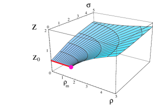
Figure 1: On the left we plot $z(\rho,\sigma)$ as given by the implicit equation (2.22). The line in this plot is the segment $z=z_{0}$ at $\sigma=0$ and $0\leq\rho\leq\rho_{m}$. On the right we plot $e^{2\Phi}$ from (2.23). In both cases we are taking $c=-1.5$.

$$e^{2\Phi(\rho,\sigma=0)}\,=\,\begin{cases}\rho^{2}\,\Big{[}\,1\,-\,{1\over\log\rho}\,+\,{1\over 2(\log\rho)^{2}}\,\Big{]}\,+\,{c\over 2(\log\rho)^{2}}\,\,,&{\rm if}\,\,\,\,\rho\geq\rho_{m}\,\,,\cr\cr e^{2z_{0}}-\rho^{2}\,\,,&{\rm if}\,\,\,\,0\leq\rho\leq\rho_{m}\,\,,\end{cases}$$ (2.27)

which, in particular means that $e^{\Phi}$ vanishes for $\sigma=0,\rho=\rho_{m}$, making the dilaton singular at that point. All these features of our solution are displayed in figure 1, which in particular shows the constant $z=z_{0}$ segment along the $\sigma=0$ axis. Taken together, all these results mean that our ${\cal N}=(2,2)$ solution can be interpreted as generated by a distribution of D5-branes smeared along the ring $\rho=\rho_{m}$, $0\leq\chi<2\pi$ and located at the $\sigma=0$ point of the $CY_{3}$. Accordingly, our solution can be regarded as the supergravity dual of a slice of the Coulomb branch of ${\cal N}=(2,2)$ two-dimensional SYM. We will confirm this interpretation in appendix A by looking at the UV and the IR behavior of our solution. Moreover, in the next subsection we will verify that $\sigma=0$ defines the SUSY locus of a D5-brane probe in our geometry.

2.2 Probe analysis

Let us now study the dynamics of a color D5-brane probe in our background. The action of such a probe is determined by the DBI+WZ action, given by:

$$S\,=\,-T_{5}\,\int d^{6}\zeta\,e^{-\Phi}\,\,\sqrt{-\det(\,\hat{G}_{6}\,+\,2\pi\alpha^{\prime}\,F)}\,+\,T_{5}\,\int\hat{C}_{6}\,\,,$$ (2.28)

where $\zeta^{a}$ ($a=0,\cdots,5$) is a set of worldvolume coordinates, $F$ is the field strength of the worldvolume gauge field, $\hat{G}_{6}$ is the induced metric and a hat over $C_{6}$ denotes its pullback to the worldvolume. The D5-brane probe we will analyze is extended along the Minkowski directions, wraps the $S^{2}\times S^{2}$ four-cycle and is located at a fixed value of the remaining coordinates. Accordingly, we shall choose our worldvolume coordinates as $\zeta^{a}\,=\,(x^{0},x^{1},\theta_{1},\phi_{1},\theta_{2},\phi_{2})$ and embed our brane at a constant value of $(\sigma,\psi,\rho,\chi)$. We will consider first the case in which the worldvolume gauge field vanishes. The induced metric for such a configuration is:

$$\hat{G}_{ab}^{(6)}\,d\zeta^{a}\,d\zeta^{b}\,=\,e^{\Phi}\,\,\Big{[}\,dx_{1,1}^{2}\,+\,{z\over m^{2}}\,\big{(}\,d\theta_{1}^{2}\,+\,\sin^{2}\theta_{1}\,d\phi_{1}^{2}\,+\,d\theta_{2}^{2}\,+\,\sin^{2}\theta_{2}\,d\phi_{2}^{2}\,\big{)}\,\Big{]}\,+\,$$

$$\qquad\qquad\qquad\qquad\qquad+\,{e^{-\Phi}\,\sigma^{2}\over m^{2}z^{2}}\,\big{[}\,\cos\theta_{1}\,d\phi_{1}\,+\,\cos\theta_{2}\,d\phi_{2}\,\big{]}^{2}\,\,.$$ (2.29)

The RR six-form potential is related to the Hodge dual of $F_{3}$ as $F_{7}=-{}^{*}F_{3}\,=\,dC_{6}$. From the first calibration condition in (2.18) one concludes that $C_{6}$ can be chosen as:

$$C_{6}\,=\,e^{-\Phi}\,{\cal K}\,\,.$$ (2.30)

By using the explicit expression of the calibration form ${\cal K}$ given in (2.15) one immediately obtains the pullback of $C_{6}$, namely:

$$\hat{C}_{6}\,=\,{e^{2\Phi}z^{2}\over m^{4}}\,\sin\theta_{1}\,\sin\theta_{2}\,d^{6}\zeta\,\,.$$ (2.31)

Plugging these results into the DBI+WZ action (2.28) one gets the value of the action for the static configuration we are considering:

$$S\,=\,-T_{5}\,\int\,d^{6}\zeta\,{z^{2}\,e^{2\Phi}\over m^{4}}\,\,\sin\theta_{1}\,\sin\theta_{2}\,\Big{[}\,\sqrt{1+\,{\sigma^{2}e^{-2\Phi}\over z^{3}}\,\big{(}\,\cot^{2}\theta_{1}\,+\,\cot^{2}\theta_{2})}\,-\,1\,\Big{]}\,\,,$$ (2.32)

which is nothing but minus the static potential between the stack of $N_{c}$ color branes that created the background and the additional probe. It is clear from (2.32) that this potential is non-vanishing except when $\sigma=0$, which confirms that this point is a zero-force supersymmetric locus inside the Calabi-Yau space. This fact can also be verified directly by means of kappa symmetry.

Let us now assume that our probe is located at $\sigma=0$ and that we switch on a worldvolume gauge field $F_{\mu\nu}$ whose only non-vanishing components are those along the Minkowski directions $x^{\mu}$. Recall that our branes can be at any point of the transverse $\mathbb{R}^{2}$ space. We will parametrize these flat directions in terms of a complex coordinate ${\cal Z}$, related to $(\rho,\chi)$ as follows:

$${\cal Z}\,=\,{1\over m}\,\rho\,e^{i\chi}\,\,,$$ (2.33)

where we have included the $1/m$ factor to absorb the one we introduced in (2.1) with our notation (notice that ${\cal Z}$ has dimensions of length). We will assume that ${\cal Z}$ only depends on $(x^{0},x^{1})$. By expanding the DBI action up to quadratic terms, we get:

$$\int_{S^{2}\times S^{2}}{\cal L}_{DBI}\Big{|}_{quadratic}=-{2(2\pi)^{4}\,(\alpha^{\prime})^{2}\,T_{5}\over m^{4}}\,z^{2}\Bigg{[}\,{1\over 2}\,{\rm Tr}\,\Big{[}F_{\mu\nu}\,F^{\mu\nu}\Big{]}+{1\over(2\pi\alpha^{\prime})^{2}}\,{\rm Tr}\,\big{[}\partial_{\mu}\,{\cal Z}^{\dagger}\,\partial^{\mu}\,{\cal Z}\,\big{]}\,\Bigg{]}\,\,,\qquad\qquad\qquad$$ (2.34)

where $z$ is evaluated at $\sigma=0$ and, in order to pass from the abelian to the non-abelian theory, we have substituted $F_{\mu\nu}\,F^{\mu\nu}\,\rightarrow\,{\rm Tr}\,\big{[}F_{\mu\nu}\,F^{\mu\nu}\big{]}$ (and similarly for ${\cal Z}$). Let us now define the complex scalar field $\Psi$ as follows:

$$\Psi\,=\,{{\cal Z}\over 2\pi\alpha^{\prime}}\,\,.$$ (2.35)

Then, the action (2.34) can be written as:

$$-{1\over 2g^{2}_{YM}}\,{\rm Tr}\,\Big{[}F_{\mu\nu}\,F^{\mu\nu}\Big{]}\,-\,{1\over g^{2}_{YM}}\,{\rm Tr}\,\big{[}\partial_{\mu}\,{\Psi}^{\dagger}\,\partial^{\mu}\,{\Psi}\,\big{]}\,\,.$$ (2.36)

where the gauge fields have the canonical normalization and the Yang-Mills coupling takes the form:

$${1\over g^{2}_{YM}}\,=\,{g_{s}\alpha^{\prime}N_{c}^{2}\over\pi}\,\,z^{2}(\rho,\sigma=0)\,\,.$$ (2.37)

From the explicit value of $z(\rho,\sigma=0)$ in (2.26) we conclude that $g_{YM}$ decreases as we move towards the UV region (large $\rho$), as expected in a non-abelian Yang-Mills theory. However, we cannot extract more specific information from (2.37) due to the fact that we do not know the precise holographic radius-energy relation. Moreover, one also has to take into account the growing of the dilaton as $\rho\rightarrow\infty$ (see (2.27)), which invalidates the supergravity approximation. This is actually a generic problem of all backgrounds generated by D5-branes (see section 4 for an alternative brane setup).

2.3 The dual of the (2,2) theory with flavor

Let us now try to extend the results of the previous subsection to the construction of a supergravity background which could encode the effects of adding flavor degrees of freedom, i.e. of fields in the fundamental representation of the gauge group. In order to perform this task we should add new (flavor) branes that introduce a new open string sector to the theory on the gravity side. These flavor branes are D5-branes that fill the Minkowski space-time and in addition are extended along a non-compact four-cycle of the Calabi-Yau threefold and sit at a fixed point in the transverse $\mathbb{R}^{2}$. Actually, the value $\rho_{Q}$ of the radial $\mathbb{R}^{2}$ coordinate $\rho$ at which the flavor branes sit in $\mathbb{R}^{2}$ parametrizes the mass $m_{Q}$ of the matter fields we are adding ($m_{Q}\sim\rho_{Q}/\sqrt{\alpha^{\prime}}$).

In order to characterize the four-dimensional submanifolds of the Calabi-Yau threefold that could be suitable to wrap a flavor brane, one should determine the embeddings of the D5-brane that preserve the four supersymmetries of the unflavored background. This analysis can be done systematically by using kappa symmetry and it is very similar to the one performed in [39] for the embeddings of D7-branes in the conifold Klebanov-Witten model (see also refs. [40, 41]). Let us skip the details of this analysis and just give the final result. Let us suppose that we have a D5-brane extended in $x^{0},x^{1}$ as well as along a four-dimensional submanifold ${\cal M}_{4}$ of the $CY_{3}$. It is quite convenient to define three complex variables $\zeta_{i}$ ($i=1,2,3$) as:

$$\zeta_{1}\,=\,\tan\Big{(}{\theta_{1}\over 2}\Big{)}\,e^{i\phi_{1}}\,\,,\qquad\zeta_{2}\,=\,\tan\Big{(}{\theta_{2}\over 2}\Big{)}\,e^{i\phi_{2}}\,\,,\qquad\zeta_{3}\,=\,\sigma\,\sin\theta_{1}\,\sin\theta_{2}\,e^{-i\psi}\,\,.$$ (2.38)

Then, the ${\cal M}_{4}$’s that correspond to a supersymmetric embedding of a D5-brane are those in which $\zeta_{1}$, $\zeta_{2}$ and $\zeta_{3}$ are constrained by a holomorphic relation. Actually, we will restrict ourselves to the case in which this relation is polynomial and ${\cal M}_{4}$ is the geometric locus of the equation:

$$\zeta_{1}^{m_{1}}\,\zeta_{2}^{m_{2}}\,\zeta_{3}^{m_{3}}\,=\,{\rm constant}\,\,,\qquad\qquad$$ (2.39)

with $m_{1}$, $m_{2}$ and $m_{3}$ being some constant exponents. When the number of flavor branes is much lower than the number $N_{c}$ of color branes, one can neglect the backreaction of the former in the geometry and treat them as probes. On the field theory side this approximation corresponds to neglecting quark loops in the ’t Hooft large $N_{c}$ expansion, i.e. to the so-called quenched approximation. In this paper we will concentrate on studying the opposite (unquenched) limit, in which the number $N_{f}$ of flavor branes is of the same order as the number $N_{c}$ of color branes. This limit is the gravity counterpart of the one considered by Veneziano [42] in gauge theories.

When $N_{f}\sim N_{c}$ the backreaction cannot be ignored and one has to consider the full coupled gravity plus branes system. Finding the general solution of the equations of motion of this coupled system for any embedding of the family (2.39) is, of course, a formidable task. For this reason we will try to find a particular class of embeddings for which the problem becomes simpler and tractable. Notice that the radial coordinate $\sigma$ and the fibered angle $\psi$ only enter in (2.39) through $\zeta_{3}$. Thus, if $m_{3}=0$, then $\sigma$ and $\psi$ are not constrained by (2.39) and they can take all possible values which, in particular, means that the cycle is non-compact as desired. If, in addition, $m_{1}$ or $m_{2}$ also vanish, the description of ${\cal M}_{4}$ in terms of the other coordinates $(\theta_{i},\phi_{i})$ greatly simplifies. Indeed, if $m_{1}=m_{3}=0$, eq. (2.39) tells us that $(\theta_{2},\phi_{2})$ are constant and $(\theta_{1},\phi_{1})$ are unconstrained. Thus, in this case, if $\xi^{\alpha}$ are a set of worldvolume coordinates, the embedding is characterized by:

$$\xi^{\alpha}\,=\,(x^{0},x^{1},\theta_{1},\phi_{1},\sigma,\psi)\,\,,\qquad\qquad(\theta_{2},\phi_{2},\rho,\chi\,\,{\rm constant})\,\,.$$ (2.40)

Similarly, when $m_{2}=m_{3}=0$ the embedding is:

$$\xi^{\alpha}\,=\,(x^{0},x^{1},\theta_{2},\phi_{2},\sigma,\psi)\,\,,\qquad\qquad(\theta_{1},\phi_{1},\rho,\chi\,\,{\rm constant})\,\,.$$ (2.41)

It is easy to check directly that superposing any number of flavor branes extended as in (2.40) and (2.41) does not break any of the supersymmetries preserved by the unflavored system. Indeed, using the fact that the total ten-dimensional chirality of the type IIB theory is fixed:

$$\Gamma^{01\cdots 9}\,\epsilon\,=\,-\Gamma_{01\cdots 9}\,\epsilon\,=\,\epsilon\,\,,$$ (2.42)

one can straightforwardly demonstrate that the projections (2.9) imply:

$$\Gamma_{012367}\tau_{1}\,\epsilon\,=\,\epsilon\,\,,\qquad\qquad\qquad\Gamma_{014567}\tau_{1}\,\epsilon\,=\,\epsilon\,\,,$$ (2.43)

which are just the conditions required by kappa symmetry to ensure that the embeddings (2.40) and (2.41) are supersymmetric.

We want to find the backreacted geometry in which the metric is still given by the ansatz (2.1). Notice that this ansatz is symmetric under the exchange of the two-spheres parametrized by $(\theta_{1},\phi_{1})$ and $(\theta_{2},\phi_{2})$. Accordingly, we will consider a configuration in which an equal number $N_{f}$ of D5-branes are extended along the two “branches” (2.40) and (2.41). Thus, the brane setup that we will consider preserves this symmetry and can be represented by means of the array:

			$\overbrace{\phantom{\qquad\qquad\qquad\qquad\qquad}}^{\text{CY}_{3}}$
	$\mathbb{R}^{1,1}$		$S^{2}$		$S^{2}$		$N_{2}$		$\mathbb{R}^{2}$
$N_{c}$ D$5$ (color)	$-$	$-$	$\bigcirc$	$\bigcirc$	$\bigcirc$	$\bigcirc$	$\cdot$	$\cdot$	$\cdot$	$\cdot$
$N_{f}$ D$5$ (flavor)	$-$	$-$	$\bigcirc$	$\bigcirc$	$\cdot$	$\cdot$	$-$	$-$	$\cdot$	$\cdot$
$N_{f}$ D$5$(flavor)	$-$	$-$	$\cdot$	$\cdot$	$\bigcirc$	$\bigcirc$	$-$	$-$	$\cdot$	$\cdot$

Contrary to what happens with the metric, in the presence of flavor branes one necessarily has to modify the ansatz of the RR three-form $F_{3}$. This is due to the fact that the branes couple to the RR fields by means of their Wess-Zumino term in the action, which leads to a modification of the Bianchi identity for $F_{3}$. To get the precise form of this modification, let us look at the WZ term of one of each flavor branes:

$$S_{WZ}^{flavor,i}\,=\,T_{5}\,\sum^{N_{f}}\,\int_{{\cal M}_{6}^{(i)}}\,\,\hat{C}_{6}\,\,,$$ (2.44)

where the index $i=1,2$ labels the two branches (2.40) and (2.41). As the embeddings are mutually supersymmetric for any value of the coordinates transverse to the flavor brane, we can homogeneously distribute the branes in some of their transverse directions. Actually, we shall locate the branes at a fixed value $\rho=\rho_{Q}$ of the radial coordinate $\rho$ (which corresponds to a fixed value of the quark mass) and we will distribute them homogeneously along their transverse angular coordinates. Moreover, when $N_{f}\rightarrow\infty$ we can substitute the discrete distribution of branes by a continuous distribution with the appropriate normalization. This approach of smearing the branes was pioneered in [19] (see also [20]) and has been applied successfully to construct several flavored backgrounds [21]-[36]. In our case, the smearing in the $i^{th}$ branch amounts to performing the substitution:

$$T_{5}\,\sum^{N_{f}}\,\int_{{\cal M}_{6}^{(i)}}\,\,\hat{C}_{6}\,\,\Rightarrow\,\,-T_{5}\,\int_{{\cal M}_{10}}\,{\rm Vol}\big{(}\,{\cal Y}_{4}^{(i)}\,\big{)}\,\wedge C_{6}\,\,,$$ (2.45)

where ${\rm Vol}\big{(}{\cal Y}_{4}^{(i)}\,\big{)}$ is the volume form of the space transverse to the $i^{th}$ branch, normalized as:

$$\int_{{\cal M}_{4}^{(i)}}\,\,{\rm Vol}\big{(}{\cal Y}_{4}^{(i)}\,\big{)}\,=\,N_{f}\,\,,$$ (2.46)

with ${\cal M}_{4}^{(i)}$ being the four-volume orthogonal to the six-dimensional worldvolume ${\cal M}_{6}^{(i)}$ of the $i^{th}$ branch. The minus sign on the right-hand side of (2.45) is due to the orientation of the worldvolume of the flavor branes. As we place the flavor branes at a fixed value $\rho_{Q}$ of the $\rho$ variable and we smear them along the other compact dimensions, one can check as in [23] that:

$${\rm Vol}\big{(}{\cal Y}_{4}^{(1)}\,\big{)}\,=\,{N_{f}\over 8\pi^{2}}\,\delta(\rho-\rho_{Q})\,d\rho\wedge d\chi\wedge\omega_{2}\,\,,\qquad{\rm Vol}\big{(}{\cal Y}_{4}^{(2)}\,\big{)}\,=\,{N_{f}\over 8\pi^{2}}\,\delta(\rho-\rho_{Q})\,d\rho\wedge d\chi\wedge\omega_{1}\,\,,$$ (2.47)

where $\omega_{1}$ and $\omega_{2}$ are the volume forms of the $(\theta_{1},\phi_{1})$ and $(\theta_{2},\phi_{2})$ two-spheres, namely:

$$\omega_{1}\,=\,\sin\theta_{1}\,d\theta_{1}\wedge d\phi_{1}\,\,,\qquad\qquad\omega_{2}\,=\,\sin\theta_{2}\,d\theta_{2}\wedge d\phi_{2}\,\,.$$ (2.48)

Given the coupling of the WZ term of the flavor branes to the $C_{6}$ potential (see (2.45)), one has the following modification of the Bianchi identity for $F_{3}$:

$$dF_{3}\,=\,2\kappa_{10}^{2}\,T_{5}\,\Omega\,\,,$$ (2.49)

where the four-form $\Omega$ is the so-called smearing form, which encodes the distribution of D5-brane charge of our setup and is given by:

$$\Omega\,=\,-{\rm Vol}\big{(}{\cal Y}_{4}^{(1)}\,\big{)}\,-\,{\rm Vol}\big{(}{\cal Y}_{4}^{(2)}\,\big{)}\,=\,-{N_{f}\over 8\pi^{2}}\,\delta(\rho-\rho_{Q})\,d\rho\wedge d\chi\wedge\,\big{(}\,\omega_{1}\,+\,\omega_{2}\,)\,\,.$$ (2.50)

Moreover, taking into account that $1/T_{5}\,=\,(2\pi)^{5}\,g_{s}\,(\alpha^{\prime})^{3}$ and $2\kappa_{(10)}^{2}\,=\,(2\pi)^{7}\,g_{s}^{2}\,(\alpha^{\prime})^{4}$, one gets:

$$dF_{3}\,=\,-{g_{s}\alpha^{\prime}N_{f}\over 2}\,\delta(\rho-\rho_{Q})\,d\rho\wedge d\chi\wedge\,\big{(}\,\omega_{1}\,+\,\omega_{2}\,\big{)}\,\,.$$ (2.51)

It is now easy to modify the ansatz for $F_{3}$ in (2.6) in such a way that (2.51) is satisfied. Indeed, one can readily verify that $F_{3}$ can be taken to be:

$$F_{3}\,=\,\Big{[}\,g\,-\,{g_{s}\alpha^{\prime}N_{f}\over 2}\,\Theta(\rho-\rho_{Q})\,\Big{]}\,d\chi\wedge(\,\omega_{1}\,+\,\omega_{2})\,+\,dg\wedge d\chi\wedge(\,d\psi+\cos\theta_{1}d\phi_{1}+\cos\theta_{2}d\phi_{2}\,)\,\,,$$ (2.52)

with $\Theta$ being the Heaviside function. As stated above, we will continue to assume that the backreacted metric has the form written in (2.1). Using for this modified ansatz the same projections as in (2.9) and the same form of the Killing spinor as in (2.10), we now get the following system of first-order BPS equations:

$$m^{2}\,\Big{[}\,g\,-\,{g_{s}\alpha^{\prime}N_{f}\over 2}\,\Theta(\rho-\rho_{Q}\,)\Big{]}\,=\,\rho\,z^{\prime}\,\,,$$

$$e^{2\Phi}\,=\,{\sigma\over z^{2}\dot{z}}\,\,,$$

$$m^{2}\,g^{\prime}\,=\,2\,e^{-2\Phi}\,\rho\,\sigma\,\dot{\Phi}\,\,,$$

$$m^{2}\,\dot{g}\,=\,-2m^{2}\,{\sigma\over z^{3}}\,e^{-2\Phi}\,\Big{[}\,g\,-\,{g_{s}\alpha^{\prime}N_{f}\over 2}\,\,\Theta(\rho-\rho_{Q}\,)\Big{]}\,\,-\,2\,{\rho\sigma\over z^{2}}\,e^{-2\Phi}\,\Phi^{\prime}\,\,.$$ (2.53)

As the set of projections imposed on the Killing spinors in this flavored case is just the same as in (2.9), any solution of the system (2.53) gives rise to a background that preserves the same four supersymmetries of the unflavored theory. Clearly, when $N_{f}=0$ or $\rho<\rho_{Q}$ the system (2.53) reduces to the one written in (2.11) for the unflavored system. Moreover, as explained in detail in appendix C, any solution of (2.53) also solves the equations of motion with source terms from the smeared flavor branes. Furthermore, as it happens for the unflavored case, we can reduce this system to the following PDE for $z(\rho,\sigma)$:

$${N_{f}\over 2N_{c}}\,\sigma\delta(\rho-\rho_{Q})\,+\,\rho\,z^{2}\,(\dot{z}\,-\,\sigma\,\ddot{z}\,)\,=\,\sigma\,(\,2\rho\,z\,\dot{z}^{2}\,+\,z^{\prime}\,+\,\rho\,z^{\prime\prime}\,)\,\,.$$ (2.54)

Notice that the effect of the flavor in (2.54) is a delta-function source located at $\rho=\rho_{Q}$.

Notice that the third equation in (2.53) implies that $g(\rho,\sigma=0)$ is also constant in this flavored case. Actually, as argued in [23] the solution should be the same as in the unflavored case for $\rho<\rho_{Q}$. Taking this into account we conclude that (2.19) also holds when $N_{f}\not=0$. Using this information it is straightforward to integrate the first equation in (2.53) and get $z(\rho,\sigma=0)$. Imposing that the solution matches the unflavored one for $\rho<\rho_{Q}$ and that is continuous at $\rho=\rho_{Q}$ one gets:

$$z(\rho,\sigma=0)\,=\,\Big{[}\,1\,-\,{N_{f}\over 2N_{c}}\,\Theta(\rho-\rho_{Q})\,\Big{]}\,\log\rho\,+\,{N_{f}\over 2N_{c}}\,\Theta(\rho-\rho_{Q})\,\log\rho_{Q}\,\,,\qquad(\rho\geq\rho_{m})\,\,.$$ (2.55)

When $N_{f}<2N_{c}$ we see from (2.55) that the addition of flavor makes $z(\rho,\sigma=0)$ grow slower with $\rho$ which, in view of (2.37) makes the UV decreasing of $g_{YM}$ smaller. Actually, this is what is expected to happen to the Yang-Mills coupling when matter degrees of freedom are added to a gauge theory. When $N_{f}>2N_{c}$ the function $z$ starts to decrease at $\rho=\rho_{Q}$ and becomes negative at some large value of $\rho$, where the solution ceases to be valid.

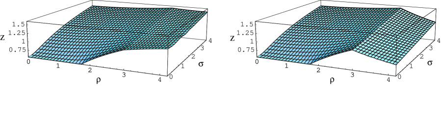
Figure 2: Plot of $z(\rho,\sigma)$ obtained by the numerical integration of (2.54) for $\rho_{Q}=3$ and $N_{f}=N_{c}$ (left) and $N_{f}=3N_{c}$ (right).

In order to evaluate $z$ for arbitrary values of $\rho$ and $\sigma$ we must integrate numerically the BPS system (2.53). In this integration we assume that the solution reduces to the unflavored one one for $\rho\leq\rho_{Q}$ and that the function $g$ is continuous at $\rho=\rho_{Q}$. Then, it follows from the first equation in (2.53) that $z^{\prime}(\rho,\sigma)$ has a discontinuity at $\rho=\rho_{Q}$ which is independent of $\sigma$ and given by:

$$z^{\prime}(\rho_{Q}+\epsilon,\sigma)\,-\,z^{\prime}(\rho_{Q}-\epsilon,\sigma)\,=\,-{N_{f}\over 2N_{c}}\,\,{1\over\rho_{Q}}\,\,.$$ (2.56)

The result of the numerical integration is shown in figure 2. Notice the characteristic wedge shape of $z(\rho,\sigma)$ near $\rho=\rho_{Q}$.

3 The dual of ${\cal N}=(1,1)$ theories

We shall now try to find a background representing D5-branes wrapped on a four-cycle with reduced supersymmetry. In particular we shall concentrate on the case in which the number of supersymmetries is two. By a simple counting argument one readily concludes that the four-cycle that the D5-branes wrap must belong to a manifold of $G_{2}$ holonomy. We are thus led to consider the following brane setup:

		$\overbrace{\phantom{\qquad\qquad\qquad\qquad\qquad}}^{\text{G}_{2}}$
	$\mathbb{R}^{1,1}$		$S^{4}$				$N_{3}$			$\mathbb{R}$
D$5$	$-$	$-$	$\bigcirc$	$\bigcirc$	$\bigcirc$	$\bigcirc$	$\cdot$	$\cdot$	$\cdot$	$\cdot$

In order to formulate a specific ansatz for the metric and the three-form of this brane arrangement, let us recall that a geometry of a non-compact manifold with $G_{2}$ holonomy with a co-associative four-cycle was found in refs. [43, 44]. Let us explicitly write this metric. We start by representing the line element of a four-sphere as:

$$d\Omega_{4}^{2}\,=\,{4\over(1+\xi^{2})^{2}}\left[d\xi^{2}+{\xi^{2}\over 4}\left((\omega^{1})^{2}+(\omega^{2})^{2}+(\omega^{3})^{2}\right)\right]\,\,,$$ (3.1)

where $-\infty<\xi<+\infty$ is a non-compact coordinate and $\omega^{i}$ ($i=1,2,3$) is a set of $SU(2)$ left-invariant one-forms satisfying $d\omega^{i}={1\over 2}\epsilon_{ijk}\,\omega^{j}\wedge\omega^{k}$. Let us in addition introduce two angular coordinates $\theta$ and $\phi$ ($0\leq\theta\leq\pi$, $0\leq\phi<2\pi$) parametrizing a two-sphere and let $E^{1}$ and $E^{2}$ be the following one forms:

$$E^{1}=d\theta+{\xi^{2}\over 1+\xi^{2}}\left(\sin\phi\,\omega^{1}-\cos\phi\,\omega^{2}\right)\,\,,$$

$$E^{2}=\sin\theta\left(d\phi-{\xi^{2}\over 1+\xi^{2}}\,\omega^{3}\right)+{\xi^{2}\over 1+\xi^{2}}\,\cos\theta\left(\cos\phi\,\omega^{1}+\sin\phi\,\omega^{2}\right)\,\,.$$ (3.2)

Then, the metric of $G_{2}$ holonomy of refs. [43, 44] can be written as:

$$ds^{2}_{7}\,=\,{(d\sigma)^{2}\over 1\,-\,{a^{4}\over\sigma^{4}}}+{\sigma^{2}\over 2}\,d\Omega_{4}^{2}+\,{\sigma^{2}\over 4}\,\,\Big{(}\,1\,-\,{a^{4}\over\sigma^{4}}\,\Big{)}\Big{[}\,(E^{1})^{2}\,+\,(E^{2})^{2}\Big{]}\,\,,$$ (3.3)

where $a$ is a real constant and the variable $\sigma$ is defined in the range $a\leq\sigma<\infty$. The geometry (3.3) is a resolved $G_{2}$ cone with a blown-up four-cycle at the tip of size $a$. Notice that the $(\theta,\phi)$ two-sphere is fibered over the four-cycle.

We will take the metric (3.3) as the starting point to formulate our ansatz for the ten-dimensional metric. First of all we add two Minkowski coordinates $x^{0,1}$ and a new non-compact coordinate $\rho$ transverse to the special holonomy manifold. Moreover, we will parametrize the size of the cycle by a function $z$, which depends on both $\sigma$ and $\rho$. The deformation of the manifold induced by the D5-brane produces a squashing between the four-cycle and the fibered $S^{2}$. We will adopt a particular ansatz for this squashing, which is just the one that is obtained when the metric is generated by uplifting from seven-dimensional gauged supergravity (see appendix A). Accordingly, let us consider a string frame metric of the form:

$$ds^{2}\,=\,e^{\Phi}\,\Big{[}\,dx^{2}_{1,1}\,+\,{z\over m^{2}}\,d\Omega_{4}^{2}\,\Big{]}\,+\,{e^{-\Phi}\over m^{2}z^{{4\over 3}}}\,\Big{[}\,d\sigma^{2}\,+\,\sigma^{2}\,\big{(}\,(E^{1})^{2}+(E^{2})^{2}\,\big{)}\,\Big{]}\,+\,{e^{-\Phi}\over m^{2}}\,(d\rho)^{2}\,\,,$$ (3.4)

where $\Phi(\rho,\sigma)$ is the dilaton and $m$ is the constant with dimension of mass written in (2.2). As in any other supergravity solution representing D5-branes, the background is endowed with a non-trivial RR three-form $F_{3}$. In order to write its expression in a compact form, let us define the one-forms ${\cal S}^{\xi}$ and ${\cal S}^{i}$ $(i=1,2,3)$ as:

$${\cal S}^{\xi}\,=\,{2\over 1+\xi^{2}}\,d\xi\,\,,$$

$${\cal S}^{1}\,=\,{\xi\over 1+\xi^{2}}\,\Big{(}\sin\phi\,\omega^{1}-\cos\phi\,\omega^{2}\Big{)}\,,$$

$${\cal S}^{2}\,=\,{\xi\over 1+\xi^{2}}\,\Big{(}\sin\theta\,\omega^{3}-\cos\theta\left(\cos\phi\,\omega^{1}+\sin\phi\,\omega^{2}\right)\Big{)}\,,$$

$${\cal S}^{3}\,=\,{\xi\over 1+\xi^{2}}\,\Big{(}-\cos\theta\,\omega^{3}-\sin\theta\left(\cos\phi\,\omega^{1}+\sin\phi\,\omega^{2}\right)\Big{)}\,.$$ (3.5)

Notice that the metric of the four-sphere can be simply written as:

$$d\Omega^{2}_{4}\,=\,\big{(}{\cal S}^{\xi}\big{)}^{2}\,+\,\big{(}{\cal S}^{1}\big{)}^{2}\,+\,\big{(}{\cal S}^{2}\big{)}^{2}\,+\,\big{(}{\cal S}^{3}\big{)}^{2}\,\,.$$ (3.6)

Let us represent $F_{3}$ in terms of a two-form potential $C_{2}$ as:

$$F_{3}\,=\,dC_{2}\,\,.$$ (3.7)

Then, we shall adopt the following ansatz for $C_{2}$:

$$C_{2}\,=\,g_{1}\,\,E^{1}\wedge E^{2}\,+\,g_{2}\,\big{(}{\cal S}^{\xi}\wedge{\cal S}^{3}\,+\,{\cal S}^{1}\wedge{\cal S}^{2}\big{)}\,\,,$$ (3.8)

where $g_{1}$ and $g_{2}$ are functions of the variables $\rho$ and $\sigma$. By using:

$$d\big{(}E^{1}\wedge E^{2}\big{)}\,=\,d\big{(}{\cal S}^{\xi}\wedge{\cal S}^{3}\,+\,{\cal S}^{1}\wedge{\cal S}^{2}\big{)}\,=\,$$

$$=\,E^{1}\wedge({\cal S}^{\xi}\wedge{\cal S}^{2}\,-\,{\cal S}^{1}\wedge{\cal S}^{3}\big{)}\,+\,E^{2}\wedge({\cal S}^{\xi}\wedge{\cal S}^{1}\,+\,{\cal S}^{2}\wedge{\cal S}^{3}\big{)}\,\,,$$ (3.9)

one finds that the field strength $F_{3}$ is given by:

$$F_{3}\,=\,\big{(}g_{1}^{\prime}\,d\rho+\,\dot{g}_{1}\,d\sigma\big{)}\wedge E^{1}\wedge E^{2}\,+\,\big{(}g_{2}^{\prime}\,d\rho+\,\dot{g}_{2}\,d\sigma\big{)}\wedge\big{(}{\cal S}^{\xi}\wedge{\cal S}^{3}\,+\,{\cal S}^{1}\wedge{\cal S}^{2}\big{)}\,+\,\qquad\qquad$$

$$\qquad\qquad\,+\,\big{(}g_{1}+g_{2}\big{)}\,\Big{[}\,E^{1}\wedge({\cal S}^{\xi}\wedge{\cal S}^{2}\,-\,{\cal S}^{1}\wedge{\cal S}^{3}\big{)}\,+\,E^{2}\wedge({\cal S}^{\xi}\wedge{\cal S}^{1}\,+\,{\cal S}^{2}\wedge{\cal S}^{3}\big{)}\,\Big{]}\,\,.\qquad\qquad$$ (3.10)

Let us now impose that our ansatz preserves two supersymmetries. As in section 2 we have to require the vanishing of the supersymmetric variations (2.7) of the dilatino and gravitino, once a certain set of projections are imposed to the Killing spinors. Specifically, let us choose the following vielbein frame basis for the metric (3.4):

$$e^{i}\,=\,e^{{\Phi\over 2}}\,dx^{i}\,\,,\qquad(i=0,1)\,\,,\qquad\qquad\qquad\qquad e^{2}\,=\,{e^{{\Phi\over 2}}\over m}\,\,\sqrt{z}\,\,{\cal S}^{\xi}\,\,,$$

$$e^{j}\,=\,{e^{{\Phi\over 2}}\over m}\,\,\sqrt{z}\,\,{\cal S}^{j-2}\,\,,\qquad(j=3,4,5)\,\,,\qquad\qquad e^{6}\,=\,{e^{-{\Phi\over 2}}\over m\,z^{{2\over 3}}}\,\,d\sigma\,\,,$$

$$e^{k}\,=\,{e^{-{\Phi\over 2}}\over m\,z^{{2\over 3}}}\,\,\sigma\,E^{k-6}\,\,,\qquad(k=7,8)\,\,,\qquad\qquad\qquad e^{9}\,=\,{e^{-{\Phi\over 2}}\over m\,}\,\,d\rho\,\,.$$ (3.11)

Then, we shall impose on the Killing spinors $\epsilon$ the following projections along the internal directions:

$$\Gamma_{25}\,\epsilon\,=\,\Gamma_{34}\,\epsilon\,=\,\Gamma_{78}\,\epsilon\,\,,$$

$$\Gamma_{45}\,\epsilon\,=\,\Gamma_{67}\,\epsilon\,\,.$$ (3.12)

In addition, we shall also require the condition that corresponds to color D5-branes extended along the Minkowski directions $x^{0}$, $x^{1}$ and along the four-cycle, namely:

$$\Gamma_{6789}\tau^{1}\,\epsilon\,=\,\epsilon\,\,.$$ (3.13)

Using the fact that the total ten-dimensional chirality is fixed (see (2.42)) this condition is equivalent to:

$$\Gamma_{012345}\tau^{1}\,\epsilon\,=\,-\epsilon\,\,.$$ (3.14)

We will assume that the Killing spinor $\epsilon$ does not depend on the Minkowski and angular coordinates. The set of BPS equations obtained in this way is:

$$\dot{\Phi}\,=\,{m^{2}\over 2}\,{z^{{2\over 3}}\,e^{2\Phi}\,\over\sigma^{2}}\,g_{1}^{\prime}\,-\,{\sigma e^{-2\Phi}\over z^{{7\over 3}}}\,\,,$$

$$\Phi^{\prime}\,=\,-{m^{2}\over 2}\,{z^{2}\,e^{2\Phi}\,\over\sigma^{2}}\,\dot{g}_{1}\,-\,{3m^{2}\over\sigma z^{{1\over 3}}}(g_{1}+g_{2})\,\,,$$

$$\dot{z}\,=\,{3\sigma\over z^{{4\over 3}}}\,e^{-2\Phi}\,\,,$$

$$z^{\prime}\,=\,{3m^{2}\over\sigma}\,z^{{2\over 3}}\,(g_{1}+g_{2})\,\,,$$

$$\dot{g}_{2}\,=\,{1\over\sigma}\,(g_{1}+g_{2})\,\,,$$

$$g_{2}^{\prime}\,=\,-{\sigma\over m^{2}z^{{2\over 3}}}\,e^{-2\Phi}\,\,.$$ (3.15)

In addition, the vanishing of the supersymmetry variation of $\psi_{M}$ implies that the derivatives with respect to $\sigma$ and $\rho$ of the Killing spinor $\epsilon$ are given by:

$$\dot{\epsilon}\,=\,{m^{2}\over 8z^{{5\over 3}}}\,\Big{[}\,2g_{2}^{\prime}\,+\,{e^{2\Phi}\,z^{{7\over 3}}\over\sigma^{2}}\,g_{1}^{\prime}\,\Big{]}\,\epsilon\,\,,$$

$$\epsilon^{\prime}\,=\,-{m^{2}\over 8z^{{1\over 3}}}\,\Big{[}\,2\dot{g}_{2}\,+\,{e^{2\Phi}\,z^{{7\over 3}}\over\sigma^{2}}\,\dot{g}_{1}\,+\,{4(g_{1}+g_{2})\over\sigma}\,\Big{]}\,\epsilon\,\,.$$ (3.16)

By comparing the right-hand sides of the two equations in (3.16) with the system (3.15), one discovers that they can be simply written as derivatives of $\Phi$, namely:

$$\dot{\epsilon}\,=\,{\dot{\Phi}\over 4}\,\epsilon\,\,,\qquad\qquad\epsilon^{\prime}\,=\,{\Phi\,^{\prime}\over 4}\,\epsilon\,\,.$$ (3.17)

It follows that $\epsilon$ must be of the form:

$$\epsilon\,=\,e^{{\Phi\over 4}}\,\epsilon_{0}\,\,,$$ (3.18)

where $\epsilon_{0}$ is a constant spinor satisfying the same projections as $\epsilon$. This means that our background is 1/16-supersymmetric, i.e. it preserves two supersymmetries which, as in the case studied in section 2, have different two-dimensional chirality, as it corresponds to a gravity dual of an ${\cal N}=(1,1)$ supersymmetric gauge theory in two dimensions.

One can verify that any solution of (3.15) solves the second-order equations of motion (see appendix C). It can be also checked that the first two equations in the system (3.15) are a consequence of the last four. Moreover, we can write a single PDE for $z(\rho,\sigma)$:

$$z^{{4\over 3}}\,\big{(}\,z\ddot{z}\,+\,{2\over 3}\,(\dot{z})^{2}\,\big{)}\,=\,{2\over 3}\,(z^{\prime})^{2}-z\,z^{\prime\prime}\,\,.$$ (3.19)

If a solution of (3.19) is known, one can use it in the system (3.15) to get the other functions of the ansatz, namely $\Phi$, $g_{1}$ and $g_{2}$.

As in the case studied in section 2, the BPS system can be recast in terms of a calibration form ${\cal K}$. Indeed, let ${\cal K}$ be defined as in (2.13)-(2.14) in terms of spinor bilinears. By using the projections (3.12)-(3.13) satisfied by the Killing spinor in this case, one gets that ${\cal K}$ can be written:

$${\cal K}\,=\,e^{01}\,\wedge\,\big{(}\,e^{2345}\,+\,e^{2367}\,+\,e^{3478}\,-\,e^{2468}\,+\,e^{3568}\,+\,e^{2578}\,+\,e^{4567}\,\big{)}\,\,,$$ (3.20)

where the $e^{a}$’s are the one-forms of the basis (3.11). Moreover, one can verify that the system (3.15) is equivalent to the calibration conditions written in (2.18) for the six-form written in (3.20).

3.1 Integration of the BPS equations

The gauged supergravity approach provides a particular solution of the PDE equation (3.19) in implicit form. The details of this solution are explained in appendix A. Let us write here the final result. The function $z(\rho,\sigma)$ is the solution of the implicit equation:

$${\rho^{2}\over z^{{1\over 3}}\,\Big{[}\,I_{{1\over 6}}\,({z\over 3})+c\,I_{-{1\over 6}}\,({z\over 3})\,\Big{]}^{2}}\,+\,{\sigma^{2}\over z^{{5\over 3}}\,\Big{[}\,I_{-{5\over 6}}\,({z\over 3})+c\,I_{{5\over 6}}\,({z\over 3})\,\Big{]}^{2}}\,=\,1\,\,,$$ (3.21)

where the $I_{n}$ are modified Bessel functions of the first kind. One can check that, indeed, this implicit function solves the PDE (3.19). In order to write the expression of the dilaton $\Phi$, let us define the function $x(z)$ as:

$$e^{x(z)}\,=\,\Bigg{[}{I_{-{5\over 6}}\,({z\over 3})+c\,I_{{5\over 6}}\,({z\over 3})\over I_{{1\over 6}}\,({z\over 3})+c\,I_{-{1\over 6}}\,({z\over 3})}\Bigg{]}^{{1\over 2}}\,\,.$$ (3.22)

Then, the dilaton $\Phi$ is given by:

$$e^{\Phi}\,=\,\sqrt{e^{6x}\,\rho^{2}\,+\,z^{-{4\over 3}}\,e^{-2x}\,\sigma^{2}}\,\,.$$ (3.23)

Let us next define the angle $\psi$ ($0\leq\psi\leq\pi)$ as:

$$\cot\psi\,=\,z^{{2\over 3}}\,e^{2x}\,\,{\rho\over\sigma}\,\,.$$ (3.24)

Then, the functions $g_{1}$ and $g_{2}$ can be written as:

$$g_{1}\,=\,{1\over m^{2}}\,\,\Big{(}\,z^{-{2\over 3}}\,e^{4x-2\Phi}\,\rho\sigma\,-\,\psi\,\Big{)}\,\,,\qquad\qquad g_{2}\,=\,{\psi\over m^{2}}\,\,.$$ (3.25)

As in the case with four supersymmetries, the interpretation of the ${\cal N}=(1,1)$ solution (3.21)-(3.25) depends crucially on the value of the integration constant $c$. We will argue in detail in appendix A that the physically sensible solution is obtained when $c<-1$. In this case the function $e^{2x(z)}$ defined in (3.22) vanishes for some value $z_{0}$ of its variable $z$, which is the solution of the following transcendental equation:

$$I_{-{5\over 6}}\Big{(}{z_{0}\over 3}\Big{)}+c\,I_{{5\over 6}}\Big{(}{z_{0}\over 3}\Big{)}=0\,\,.$$ (3.26)

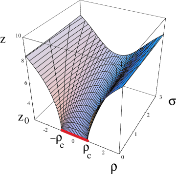
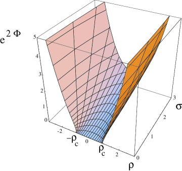
Figure 3: Plots of $z(\rho,\sigma)$ (left) and $e^{2\Phi}$ (right) obtained from (3.21) and (3.23). In both cases we have taken $c=-1.5$. On the left plot we have represented by a line the segment $z=z_{0}$, $-\rho_{c}\leq\rho\leq\rho_{c}$ in the $\sigma=0$ plane.

By inspecting (3.21) we deduce that $\sigma=0$ when $z=z_{0}$. Actually, from the explicit plot of the function $z(\rho,\sigma)$ (see figure (3)) we conclude that $z=z_{0}$ defines a segment in the $\sigma=0$ axis. This segment is characterized by the conditions $\sigma=0,\,\,-\rho_{c}\leq\rho\leq\rho_{c}$, with:

$$\rho_{c}=z_{0}^{{1\over 6}}\,\Big{|}\,I_{{1\over 6}}\,({z_{0}\over 3})+c\,I_{-{1\over 6}}\,({z_{0}\over 3})\,\Big{|}\,\,.$$ (3.27)

One can also verify that $e^{\Phi}$ vanishes along this constant $z=z_{0}$ segment. Thus our solution has a linear distribution of singularities. One can check that these singularities are good in the sense of [3] (see appendix A). Therefore, our solution can naturally be interpreted as being generated by a linear distribution of D5-branes, smeared along a finite segment on the direction of the coordinate $\rho$ orthogonal to the $G_{2}$ holonomy manifold (see appendix A for a more detailed study). Accordingly, the solution (3.21)-(3.25) can be regarded as giving the gravity dual of a slice of the Coulomb branch of ${\cal N}=(1,1)$ SYM. We will further check this statement in the next subsection by means of a probe computation.

3.2 Probe analysis

Let us now consider a D5-brane probe extended along the Minkowski directions and wrapping the four-sphere. The dynamics of such a probe is governed by the action (2.28). In order to select an appropriate set of worldvolume coordinates, let us parametrize the left-invariant one-forms $\omega^{i}$ appearing in $d\Omega_{4}^{2}$ by means of three angles $\tilde{\theta}$, $\tilde{\varphi}$ and $\tilde{\psi}$ as follows:

$$\omega^{1}\,=\,\cos\tilde{\psi}\,d\tilde{\theta}\,-\,\sin\tilde{\psi}\,\sin\tilde{\theta}\,d\tilde{\varphi}\,\,,$$

$$\omega^{2}\,=\,\sin\tilde{\psi}\,d\tilde{\theta}\,+\,\cos\tilde{\psi}\,\sin\tilde{\theta}\,d\tilde{\varphi}\,\,,$$

$$\omega^{3}\,=\,d\tilde{\psi}\,-\,\cos\tilde{\theta}\,d\tilde{\varphi}\,\,,$$ (3.28)

with $0\leq\tilde{\theta}\leq\pi$, $0\leq\tilde{\varphi}<2\pi$, $0\leq\tilde{\psi}<4\pi$. Given this parametrization, we will choose $\zeta^{a}\,=\,(x^{0},x^{1},\xi,\tilde{\theta},\tilde{\varphi},\tilde{\psi})$ as our set of worldvolume coordinates and we will assume that the remaining ten-dimensional coordinates ($\sigma$, $\theta$, $\phi$ and $\rho$) are constant. In order to write the induced metric for this embedding, let us point out that, as follows from their definition, the one-forms $E^{1}$ and $E^{2}$ can be written as:

$$E^{1}\,=\,d\theta\,+\,\xi\,{\cal S}^{1}\,\,,\qquad\qquad E^{2}\,=\,\sin\theta\,d\phi\,-\,\xi\,{\cal S}^{2}\,\,,$$ (3.29)

where ${\cal S}^{1}$ and ${\cal S}^{2}$ are the one-forms defined in (3.5). Then, the pullback of $E^{1,2}$ to the worldvolume for our particular embedding is related to those of ${\cal S}^{1}$ and ${\cal S}^{2}$, namely $\hat{E}^{1}=\xi\,\hat{\cal S}^{1}$, $\hat{E}^{2}=-\xi\,\hat{\cal S}^{2}$. Hence, it follows that the induced metric, in string frame, becomes:

$$\hat{G}^{(6)}_{ab}\,d\zeta^{a}\,d\zeta^{b}\,=\,e^{\Phi}\,dx^{2}_{1,1}\,+\,{e^{\Phi}\,z\over m^{2}}\,\Big{(}\,1\,+\,{\sigma^{2}\over z^{{7\over 3}}\,e^{2\Phi}}\,\,\xi^{2}\,\Big{)}\,\Big{(}\,\big{(}\hat{\cal S}^{1}\big{)}^{2}\,+\,\big{(}\hat{\cal S}^{2}\big{)}^{2}\,\Big{)}\,+\,{e^{\Phi}\,z\over m^{2}}\,\Big{(}\,\big{(}\hat{\cal S}^{3}\big{)}^{2}\,+\,\big{(}\hat{\cal S}^{\xi}\big{)}^{2}\,\Big{)}\,\,.$$ (3.30)

We will first consider the configuration in which the worldvolume gauge field $F$ vanishes. The determinant of the induced metric entering the DBI action in this case is just:

$$\sqrt{-\det\hat{G}_{6}}\,=\,{2z^{2}\,e^{3\Phi}\over m^{4}}\,\,\Big{(}\,1\,+\,{\sigma^{2}\over z^{{7\over 3}}\,e^{2\Phi}}\,\,\xi^{2}\,\Big{)}\,{\xi^{3}\sin\tilde{\theta}\over(1+\xi^{2})^{4}}\,\,.$$ (3.31)

Therefore, the DBI term in the action is:

$$S_{DBI}\,=\,-{2T_{5}\over m^{4}}\,\int d^{6}\zeta\,\,z^{2}\,e^{2\Phi}\,\Big{(}\,1\,+\,{\sigma^{2}\over z^{{7\over 3}}\,e^{2\Phi}}\,\,\xi^{2}\,\Big{)}\,{\xi^{3}\sin\tilde{\theta}\over(1+\xi^{2})^{4}}\,\,.$$ (3.32)

In the Wess-Zumino term of the action $\hat{C}_{6}$ is the pullback of the RR six-form potential which can be chosen in terms of the calibration form as in (2.30). From the explicit expression of ${\cal K}$ in (3.20), we get the pullback of $C_{6}$, namely:

$$\hat{C}_{6}\,=\,{2z^{2}\,e^{2\Phi}\,\xi^{3}\sin\tilde{\theta}\over m^{4}\,(1+\xi^{2})^{4}}\,\Big{(}\,1\,-\,{\sigma^{2}\xi^{2}\over z^{{7\over 3}}\,e^{2\Phi}}\,\Big{)}\,d^{6}\zeta\,\,.$$ (3.33)

By adding the DBI and WZ contributions we get:

$$S\,=\,-{4T_{5}\over m^{4}}\,\,\int d^{6}\zeta\,\,\sigma^{2}\,{\xi^{5}\sin\tilde{\theta}\over(1+\xi^{2})^{4}\,z^{{1\over 3}}}\,\,,$$ (3.34)

which is just minus the static potential between the stack of color branes and the additional probe. This potential is vanishing for $\sigma=0$, which is the no-force locus of the branes in the internal manifold. It can easily be checked by using kappa symmetry that this $\sigma=0$ configuration is also supersymmetric.

Let us next assume that we are at the $\sigma=0$ point and that we switch on a worldvolume gauge field $F$ such that its only non-vanishing components are directed along the unwrapped Minkowski directions $x^{0,1}$. Following the same steps as in subsection 2.2 one can expand the DBI action up to quadratic order and find the expression of the Yang-Mills coupling. One gets:

$${1\over g_{YM}^{2}}\,=\,{g_{s}\,\alpha^{\prime}\,N_{c}^{2}\over 6\pi}\,z^{2}(\rho,\sigma=0)\,\,.$$ (3.35)

The function $z(\rho,\sigma=0)$ can be obtained from the implicit relation (3.21). As is clear from the plot in figure 3, $z(\rho,\sigma=0)$ grows when $\rho$ is large which, according to (3.35), makes $g_{YM}$ decrease in the UV, as expected. However, as in the case with four supersymmetries, the dilaton blows up at $\rho\rightarrow\infty$ and the behavior of the solution in the deep UV region is not trustable.

3.3 Addition of flavor

Let us now consider the addition of backreacting flavor D5-branes to the previous ${\cal N}=(1,1)$ background. These flavor branes should be non-compact (extended along the $\sigma$ direction) and should be extended in such a way that they do not further break the supersymmetry. Actually, we will be able to find a set of suitable deformations of the unflavored background without determining previously the family of supersymmetric embeddings of the flavor branes. In principle one should use kappa symmetry to find the precise shape of these D5-branes in the ${\cal N}=(1,1)$ background. However, this analysis is quite involved and we will not attempt to perform it directly. Instead, we will try to find directly the four-form charge density distribution for the system of extended calibrated sources, $\Omega$, which is compatible with our metric ansatz (3.4) and preserves all the supersymmetries of the unflavored system. We will find a general expression of $\Omega$ which we will subsequently restrict to a particular case with interesting properties. The corresponding background metric for this $\Omega$ can be computed by numerical integration of the system of BPS equations. In subsection 3.3.1 we will find a set of supersymmetric embeddings for the flavor branes and we will argue that the $\Omega$ found previously by studying the compatibility of SUSY with our ansatz contains the density distribution which results after averaging over these embeddings in a suitable way.

Recall that, due to the WZ term of the action for the smeared brane system, $T_{5}\int\Omega\wedge C_{6}$, the Bianchi identity is violated as:

$$dF_{3}\,=\,2\kappa_{10}^{2}\,T_{5}\,\Omega\,\,.$$ (3.36)

As in the ${\cal N}=(2,2)$ case, we will place our flavor branes at a fixed value $\rho_{Q}$ in the $\rho$ coordinate ($\rho_{Q}$ being proportional to the quark mass). Thus, the smearing form $\Omega$ should contain $\delta(\rho-\rho_{Q})$ in its expression. Moreover, it is clear from (3.36) that $d\Omega=0$. These last two conditions are satisfied if $\Omega$ is of the form:

$$2\kappa_{10}^{2}\,T_{5}\,\Omega\,=\,\delta(\rho-\rho_{Q})\,d\rho\,\wedge\,d\Lambda\,\,,$$ (3.37)

where $\Lambda$ is a two-form depending on $\sigma$ and on the angular coordinates. Notice that we can represent $F_{3}$ satisfying (3.36) as:

$$F_{3}\,=\,dC_{2}\,+\,f_{3}\,\,,$$ (3.38)

where $df_{3}=2\kappa_{10}^{2}\,T_{5}\,\Omega$. Clearly, one can take $f_{3}$ to be given by:

$$f_{3}\,=\,\Theta(\rho-\rho_{Q})\,d\Lambda\,\,.$$ (3.39)

Thus, the total RR three-form field strength is just:

$$F_{3}\,=\,dC_{2}\,+\,\Theta(\rho-\rho_{Q})\,d\Lambda\,\,.$$ (3.40)

From the expression (3.40) of $F_{3}$ the similarity between the two-form $\Lambda$ and the RR potential $C_{2}$ is quite evident. We will assume in this flavored case that $C_{2}$ is still given by the ansatz (3.8). It is thus natural to adopt a similar ansatz for $\Omega$, namely:

$$\Lambda\,=\,L_{1}(\sigma)\,E^{1}\wedge E^{2}\,+\,L_{2}(\sigma)\,\Big{[}\,{\cal S}^{\xi}\wedge{\cal S}^{3}\,+\,{\cal S}^{1}\wedge{\cal S}^{2}\,\Big{]}\,\,,$$ (3.41)

where $L_{1}$ and $L_{2}$ are functions of the coordinate $\sigma$ to be determined. Notice that the resulting value of the smearing form $\Omega$ is given by:

$$\Omega\,=\,{\delta(\rho-\rho_{Q})\over 2\kappa_{10}^{2}\,T_{5}}\,d\rho\wedge\,\Bigg{[}(L_{1}+L_{2})\,\Big{[}\,E^{1}\wedge({\cal S}^{\xi}\wedge{\cal S}^{2}\,-\,{\cal S}^{1}\wedge{\cal S}^{3}\big{)}\,+\,E^{2}\wedge({\cal S}^{\xi}\wedge{\cal S}^{1}\,+\,{\cal S}^{2}\wedge{\cal S}^{3}\big{)}\,\Big{]}\,+\,$$

$$\qquad\qquad\qquad\qquad\qquad+\dot{L}_{1}\,d\sigma\,\wedge\,E^{1}\wedge E^{2}\,+\,\dot{L}_{2}\,d\sigma\wedge\Big{[}\,{\cal S}^{\xi}\wedge{\cal S}^{3}\,+\,{\cal S}^{1}\wedge{\cal S}^{2}\,\Big{]}\,\Bigg{]}\,\,.$$ (3.42)

Moreover, if $C_{2}$ is parametrized in terms of the functions $g_{1}$ and $g_{2}$ as in (3.8), the total RR three-form $F_{3}$ for the flavored background can be written as:

$$F_{3}\,=\,\big{[}g_{1}^{\prime}\,d\rho+\,\big{(}\dot{g}_{1}\,+\,\dot{L}_{1}\,\Theta(\rho-\rho_{q})\big{)}d\sigma\big{]}\,\wedge E^{1}\wedge E^{2}\,+\,$$

$$+\big{[}g_{2}^{\prime}\,d\rho+\,\big{(}\dot{g}_{2}\,+\,\dot{L}_{2}\,\Theta(\rho-\rho_{q})\,\big{)}d\sigma\big{]}\wedge\big{(}{\cal S}^{\xi}\wedge{\cal S}^{3}\,+\,{\cal S}^{1}\wedge{\cal S}^{2}\big{)}\,+\,$$ (3.43)

$$\,+\,\big{(}g_{1}+g_{2}+(L_{1}+L_{2})\Theta(\rho-\rho_{q})\big{)}\,\Big{[}\,E^{1}\wedge({\cal S}^{\xi}\wedge{\cal S}^{2}\,-\,{\cal S}^{1}\wedge{\cal S}^{3}\big{)}\,+\,E^{2}\wedge({\cal S}^{\xi}\wedge{\cal S}^{1}\,+\,{\cal S}^{2}\wedge{\cal S}^{3}\big{)}\,\Big{]}\,\,.$$

It is clear from this expression that the flavored BPS system can be obtained from the unflavored one in (3.15) by means of the substitution:

$$\dot{g}_{i}\rightarrow\dot{g}_{i}\,+\,\dot{L}_{i}\,\Theta(\rho-\rho_{Q})\,\,,\qquad(i=1,2)\,\,,$$

$$g_{1}+g_{2}\rightarrow g_{1}+g_{2}\,+\,(L_{1}+L_{2})\,\Theta(\rho-\rho_{Q})\,\,.$$ (3.44)

One gets:

$$\dot{\Phi}\,=\,{m^{2}\over 2}\,{z^{{2\over 3}}\,e^{2\Phi}\,\over\sigma^{2}}\,g_{1}^{\prime}\,-\,{\sigma e^{-2\Phi}\over z^{{7\over 3}}}\,\,,$$

$$\Phi^{\prime}\,=\,-{m^{2}\over 2}\,{z^{2}\,e^{2\Phi}\,\over\sigma^{2}}\,\big{[}\,\dot{g}_{1}\,+\,\dot{L}_{1}\,\Theta(\rho-\rho_{Q})\,\big{]}\,-\,{3m^{2}\over\sigma z^{{1\over 3}}}\big{[}\,g_{1}+g_{2}+(L_{1}+L_{2})\Theta(\rho-\rho_{Q})\,\big{]}\,\,,$$

$$\dot{z}\,=\,{3\sigma\over z^{{4\over 3}}}\,e^{-2\Phi}\,\,,$$

$$z^{\prime}\,=\,{3m^{2}\over\sigma}\,z^{{2\over 3}}\,\big{[}\,g_{1}+g_{2}+(L_{1}+L_{2})\Theta(\rho-\rho_{Q})\,\big{]}\,\,,$$

$$\dot{g}_{2}\,=\,{1\over\sigma}\,\big{[}\,g_{1}+g_{2}+(L_{1}+L_{2})\Theta(\rho-\rho_{Q})\,\big{]}\,-\,\dot{L}_{2}\,\Theta(\rho-\rho_{Q})\,,$$

$$g_{2}^{\prime}\,=\,-{\sigma\over m^{2}z^{{2\over 3}}}\,e^{-2\Phi}\,\,.$$ (3.45)

By analyzing the system (3.45) one easily discovers that the $(\rho,\sigma)$ crossed derivatives of the functions $g_{1}$ and $g_{2}$ are not equal. Indeed, one can prove that:

$$\partial_{\rho}\,\dot{g}_{1}\,-\,\partial_{\sigma}\,g_{1}^{\prime}\,=\,\partial_{\sigma}\,g_{2}^{\prime}\,-\,\partial_{\rho}\,\dot{g}_{2}\,=\,-{1\over\sigma}\,\big{[}\,L_{1}\,+\,L_{2}\,-\,\sigma\dot{L}_{2}\,\big{]}\,\delta(\rho-\rho_{Q})\,\,,$$ (3.46)

which, after all, is not surprising since the first derivatives of $g_{1}$ and $g_{2}$ are potentially singular at $\rho=\rho_{Q}$ according to the system (3.45). Notice that this would make $d^{2}C_{2}\not=0$ and our stating point equation (3.36) would not be satisfied for the $\Omega$ written in (3.42). In order to avoid dealing with this unwanted singularity, we will require the vanishing of the right-hand side of (3.46), which is equivalent to imposing that $L_{1}$ and $L_{2}$ satisfy the differential equation:

$$\dot{L}_{2}\,=\,{1\over\sigma}\,\big{(}\,L_{1}\,+\,L_{2}\,\big{)}\,\,.$$ (3.47)

Notice also that, if equation (3.47) holds, the equation for $\dot{g}_{2}$ becomes:

$$\dot{g}_{2}\,=\,{1\over\sigma}\,\big{[}\,g_{1}+g_{2}\,\big{]}\,\,,$$ (3.48)

and the potentially singular term for $\dot{g}_{2}$ at $\rho=\rho_{Q}$ disappears. Furthermore, as shown in appendix C, any solution of (3.45) with $L_{1}$ and $L_{2}$ satisfying (3.47) also solves the equations of motion of the gravity plus (smeared) branes system. Moreover, as in the unflavored system, one can write a single PDE for the function $z(\rho,\sigma)$, which now has a source term parametrized by $L_{1}\,+\,L_{2}$, namely:

$$z^{{4\over 3}}\,\big{(}\,z\ddot{z}\,+\,{2\over 3}\,(\dot{z})^{2}\,\big{)}\,=\,{2\over 3}\,(z^{\prime})^{2}-z\,z^{\prime\prime}\,-\,{3m^{2}(L_{1}(\sigma)\,+\,L_{2}(\sigma))\over\sigma}\,z^{{5\over 3}}\,\delta(\rho-\rho_{Q})\,\,.$$ (3.49)

Furthermore, one can verify that the calibration conditions (2.18) reduce to the system (3.45) when the new ansatz (3.43) for $F_{3}$ is adopted.

Notice that one can use the compatibility condition (3.47) to obtain the function $L_{2}(\sigma)$ in terms of $L_{1}(\sigma)$. Indeed, one can easily integrate (3.47) by applying the method of variation of constants, with the result:

$$L_{2}(\sigma)\,=\,\Big{[}\,A\,+\,\int_{\sigma_{0}}^{\sigma}\,\,d\zeta\,\,{L_{1}(\zeta)\over\zeta^{2}}\,\,\,\Big{]}\,\sigma\,\,,$$ (3.50)

where $A$ and $\sigma_{0}$ are constants. Eq. (3.50) is not enough to determine $L_{1}$ and $L_{2}$. For this reason one has to find some other physical conditions that could be used to constrain these functions. Recall that $\Omega$ parametrizes the volume transverse to the flavor branes, on which we smear them to produce a continuous distribution. Its Hodge dual ${}^{*}\Omega$ is a six-form with components parallel to the worldvolume of the flavor branes. Color and flavor branes should not overlap in the internal space. It is thus natural to require the vanishing of the pullback of ${}^{*}\Omega$ to the worldvolume of the color branes, namely:

$${}^{*}\,\Omega{|_{color\,wv}}\,=\,0\,\,.$$ (3.51)

Recall from the analysis of subsection 3.2 that the color branes are located at $\sigma={\rm constant}=0$ and their angular embedding is such that the pullback of the forms $E^{1}$ and $E^{2}$ is such that $\hat{E}^{1}=\xi\,\hat{\cal S}^{1}$ and $\hat{E}^{2}=-\xi\,\hat{\cal S}^{2}$. By computing explicitly the pullback of ${}^{*}\Omega$ to this submanifold, we get:

$${}^{*}\,\Omega{|_{color\,wv}}\,=\,{m^{4}\over 2\kappa_{10}^{2}\,T_{5}}\,\,\delta(\rho-\rho_{Q})\,\Big{[}\,e^{3\Phi}\,z^{4}\,\,{\dot{L}_{1}\over\sigma^{2}}\,-\,{e^{\Phi}\over z^{{2\over 3}}}\,\xi^{2}\,\sigma^{2}\,\dot{L}_{2}\,\Big{]}_{\sigma=0}\,\,dx^{0}\wedge dx^{1}\wedge{\rm Vol}(S^{4})\,\,.$$ (3.52)

Thus, to impose the condition (3.51) one has to require:

$${\dot{L}_{1}\over\sigma^{2}}{\Big{|}_{\sigma=0}}\,=\,\sigma^{2}\,\dot{L}_{2}\big{|}_{\sigma=0}\,=\,0\,\,,$$ (3.53)

which constrain the behavior of $L_{1}$ and $L_{2}$ near $\sigma=0$. Actually, the condition on $L_{1}$ just means that, if we assume that $L_{1}\sim\sigma^{\beta}$ near $\sigma=0$, then necessarily $\beta>3$. In fact, assuming this power behavior of $L_{1}$, it is straightforward to use (3.50) to get $L_{1}$ and $L_{2}$, namely:

$$L_{1}\,=\,B\,\sigma^{\beta}\,\,,\qquad L_{2}\,=\,A\sigma\,+\,{B\over\beta-1}\,\,\sigma^{\beta-1}\,\,,\qquad(\beta>3)\,\,.$$ (3.54)

Another test that the smearing form $\Omega$ must pass can be obtained by looking at the the DBI term of the action of the system of smeared branes. Taking into account that, for a SUSY configuration, the induced volume form is just the pullback of the calibration form ${\cal K}$ and that the smearing is performed just by taking the wedge product with $\Omega$, this action takes the form:

$$S^{flavor}_{DBI}\,=\,-T_{5}\,\int_{{\cal M}_{10}}\,e^{-{\Phi}}\,\Omega\wedge{\cal K}\,\,.$$ (3.55)

The ten-form $\Omega\wedge{\cal K}$ can be explicitly computed from (3.42) and (3.20), with the result:

$$\Omega\wedge{\cal K}\,=\,-{m^{4}\over 2\kappa_{10}^{2}\,T_{5}}\,\,z^{-{1\over 3}}\,\,\Big{[}\,6\dot{L}_{2}\,+\,z^{{7\over 3}}\,e^{2\Phi}\,\,{\dot{L}_{1}\over\sigma^{2}}\,\Big{]}\,\delta(\rho-\rho_{Q})\,\,{\rm Vol}\,({\cal M}_{10})\,\,.$$ (3.56)

Notice that $\Omega\wedge{\cal K}$ can be interpreted as the mass distribution of the system of flavor branes which, being a ten-form in a ten-dimensional space, is proportional to the volume form ${\rm Vol}\,({\cal M}_{10})$ of the ten-dimensional manifold. The function multiplying ${\rm Vol}\,({\cal M}_{10})$ in (3.56) represents the mass density of the $\rho=\rho_{Q}$ slice of the space in which we are smearing the flavor branes. Notice also that our conditions (3.53) ensure the regularity of $\Omega\wedge{\cal K}$ at $\sigma=0$. Moreover, from a physical point of view one should require that the mass distribution $\Omega\wedge{\cal K}$ integrated over any portion of ${\cal M}_{10}$ always gives a positive number. This positivity condition is fulfilled if the function multiplying ${\rm Vol}\,({\cal M}_{10})$ is everywhere positive. One can check that this is the case when $L_{1}$ and $L_{2}$ are given by (3.54) if both constants $A$ and $B$ are negative. Actually, there is a solution of those written in (3.54) that is particularly simple and appealing, namely:

$$L_{1}=0\,\,,\qquad\,\,L_{2}\,=\,A\,\,\sigma\,\,.$$ (3.57)

In order to explore the properties of this solution, let us parametrize the constant $A$ as:

$$A\,=\,-2\kappa_{10}^{2}\,T_{5}\,\,{3n_{f}\over 2\pi}\,\,,$$ (3.58)

where we introduced the factor $2\kappa_{10}^{2}\,T_{5}$ to absorb the one we have introduced in the definition of $L_{1}$ and $L_{2}$ in (3.42) and the remaining factors have been introduced for convenience. The constant $n_{f}$ characterizes the density of flavor branes of our setup (see subsection 3.3.1). Notice that, in this case, $\Omega$ can be neatly written in terms of the one-forms of the frame basis (3.11) as:

$$\Omega\,=\,-{3n_{f}\over 2\pi}\,\,{m^{4}\over z^{{1\over 3}}}\,\delta(\rho-\rho_{Q})\,\,e^{9}\wedge\,\Big{[}\,e^{7}\wedge(e^{2}\wedge e^{4}-e^{3}\wedge e^{5})\,+\,e^{8}\wedge(e^{2}\wedge e^{3}+e^{4}\wedge e^{5})\,+\,$$

$$\qquad\qquad\qquad\qquad\qquad\qquad\qquad+\,e^{6}\wedge(e^{2}\wedge e^{5}+e^{3}\wedge e^{4})\,\Big{]}\,\,.$$ (3.59)

Moreover, the mass distribution is just given by:

$$\Omega\wedge{\cal K}\,=\,{9n_{f}\over\pi}\,m^{4}\,\,\,z^{-{1\over 3}}\,\delta(\rho-\rho_{Q})\,\,{\rm Vol}\,({\cal M}_{10})\,\,,$$ (3.60)

and the PDE equation (3.49) takes the form:

$$z^{{4\over 3}}\,\big{(}\,z\ddot{z}\,+\,{2\over 3}\,(\dot{z})^{2}\,\big{)}\,=\,{2\over 3}\,(z^{\prime})^{2}-z\,z^{\prime\prime}\,+\,{9\pi n_{f}\over N_{c}}\,z^{{5\over 3}}\,\delta(\rho-\rho_{Q})\,\,.$$ (3.61)

Notice that the source term in (3.61) is not singular at $\sigma=0$. Moreover, from the fourth equation in the flavored BPS system (3.45), we get that:

$$z^{\prime}\,=\,3m^{2}\,z^{{3\over 3}}\,\Big{[}\,{g_{1}+g_{2}\over\sigma}\,-\,6\pi g_{s}\alpha^{\prime}n_{f}\,\Theta(\rho-\rho_{Q})\,\Big{]}\,\,.$$ (3.62)

In order to integrate (3.61) we assume that $z(\rho,\sigma)$ is given by the unflavored solution (3.21) for $\rho\leq\rho_{Q}$, while at $\rho=\rho_{Q}$ the derivative of $z$ with respect to $\rho$ jumps in the form dictated by (3.62), namely:

$$z^{\prime}(\rho_{Q}+\epsilon,\sigma)\,-\,z^{\prime}(\rho_{Q}-\epsilon,\sigma)\,=\,-{18\pi n_{f}\over N_{c}}\,\,z^{{3\over 3}}(\rho_{Q},\sigma)\,\,.$$ (3.63)

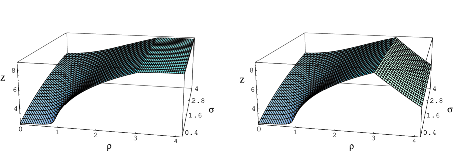
Figure 4: Plot of $z(\rho,\sigma)$ obtained by the numerical integration of (3.61) for $\rho_{Q}=3$ and $x\equiv{18\pi n_{f}\over N_{c}}=0.2$ (left) and $x=1$ (right).

In figure 4 we have plotted the function $z(\rho,\sigma)$, resulting from the numerical integration of the PDE (3.61), for two different values of $n_{f}$. Notice the similarity with the results obtained for the flavored system with four supersymmetries (see figure 2).

3.3.1 Microscopic analysis of the smearing

The smearing form $\Omega$ is the flavor density distribution that should be obtained after averaging over a continuous set of supersymmetric brane embeddings. For the case at hand we have not been able to find the most general embedding of a flavor brane that preserves all the supersymmetries of the unflavored background. However, we have been able to find a set of such embeddings and we will argue that, after performing a suitable average, they give rise to some of the components of the smearing density (3.59). In order to illustrate this fact let us consider a D5-brane whose worldvolume is parametrized by the following set of coordinates:

$$\zeta^{a}\,=\,(x^{0},x^{1},\xi,\tilde{\psi},\sigma,\phi)\,\,.$$ (3.64)

Moreover, we will assume that the embedding of the brane in the ten-dimensional spacetime is given by:

$$\theta=\theta(\sigma)\,\,,\qquad\qquad\tilde{\theta}\,,\,\tilde{\varphi}={\rm constant}\,\,,\qquad\rho=\rho_{Q}\,\,,$$ (3.65)

where $\theta(\sigma)$ is a function to be determined and $\tilde{\theta}$, $\tilde{\varphi}$ and $\tilde{\psi}$ are the three angles which parametrize the $SU(2)$ left-invariant one-forms $\omega^{1}$, $\omega^{2}$ and $\omega^{3}$ (see (3.28)). By using the kappa symmetry condition $\Gamma_{\kappa}\,\epsilon\,=\,\epsilon$ one can easily prove that, in order to preserve the two supersymmetries of the background, the function $\theta(\sigma)$ must satisfy the following differential equation:

$$\sigma\partial_{\sigma}\theta\,=\,\cot\theta\,\,.$$ (3.66)

The integration of this equation yields:

$$\cos\theta\,=\,{\sigma_{*}\over\sigma}\,\,,$$ (3.67)

with $\sigma^{*}$ being a constant. Notice that in (3.67) $\sigma\geq|\sigma_{*}|$, i.e. $|\sigma_{*}|$ is the minimal value of the coordinate $\sigma$ along the brane (for which $\theta=0,\pi$). Notice that, for the ansatz (3.65), the brane is embedded in the $S^{4}$ in such a way that the pullback of the one-forms $\omega^{1}$ and $\omega^{2}$ vanish, while $\hat{\omega}^{3}=d\tilde{\psi}$. Therefore, the induced metric on the brane worldvolume takes the form:

$$e^{\Phi}\,dx^{2}_{1,1}\,+\,{ze^{\Phi}\over m^{2}}\,\,{1\over(1+\xi^{2})^{2}}\,\,\Big{[}4\,d\xi^{2}+\xi^{2}\,d\tilde{\psi}^{2}\,\Big{]}+{e^{-\Phi}\over m^{2}z^{{4\over 3}}}\,\Big{[}{d\sigma^{2}\over\sin^{2}\theta}\,+\,\sigma^{2}\,\sin^{2}\theta\big{(}d\phi\,-\,{\xi^{2}\over 1+\xi^{2}}\,d\tilde{\psi}\big{)}^{2}\,\Bigg{]}\,\,.\qquad\qquad$$ (3.68)

As a check of the supersymmetric nature of these embeddings one can verify that the induced volume form corresponding to the metric (3.68) is equal to the pullback of the calibration form (3.20). Notice also that these embeddings determine a two-sphere inside the $S^{4}$.

The configuration of the flavor brane just found has a neat interpretation when one looks in detail at the structure of the normal bundle $N_{3}$ spanned by the coordinates $(\sigma,\theta,\phi)$. By inspecting the metric (3.4) one realizes that $N_{3}$ is a three-dimensional flat space $\mathbb{R}^{3}$ fibered over the four-cycle. Accordingly, let us introduce the following set of cartesian coordinates for $N_{3}$:

$$z^{1}\,=\,\sigma\sin\theta\cos\phi\,\,,\qquad z^{2}\,=\,\sigma\sin\theta\sin\phi\,\,,\qquad z^{3}\,=\,\sigma\cos\theta\,\,.$$ (3.69)

In terms of these coordinates, the embeddings just found correspond to the plane:

$$z^{3}\,=\,\sigma_{*}\,\,.$$ (3.70)

Notice that we have found a family of configurations parametrized by the constant values of $\tilde{\theta}$, $\tilde{\varphi}$ and $\sigma_{*}$ at $\rho=\rho_{Q}$. By changing $\tilde{\theta}$, $\tilde{\varphi}$ we select a different $S^{2}$ inside the $S^{4}$. Moreover, it is clear from (3.70) that changing $\sigma_{*}$ corresponds to choosing a plane $z^{3}\,=\,$constant in $N_{3}$. Let us suppose that we consider a set of branes embedded in this way that are homogeneously distributed within the $S^{4}$ and $N_{3}$. The resulting distribution form $\Gamma$ should be proportional to the volume element of the space transverse to the branes, which is two-dimensional within the $S^{4}$ and one-dimensional inside the $N_{3}$. Accordingly, let us write $\Gamma$ in factorized form as:

$$\Gamma\,=\,\delta(\rho-\rho_{Q})\,d\rho\wedge\Gamma_{1}\wedge\Gamma_{2}\,\,,$$ (3.71)

with $\Gamma_{1}$ and $\Gamma_{2}$ being the contributions of the $S^{4}$ and $N_{3}$ respectively. For the embeddings (3.65) the transverse directions inside the $S^{4}$ are those spanned by the one-forms $\omega^{1}$ and $\omega^{2}$. By looking at the line element of $S^{4}$ it is easy to get the corresponding transverse volume form, namely:

$$\Gamma_{1}\,=\,{3\over 2\pi}\,\,{\xi^{2}\over(1+\xi^{2})^{2}}\,\omega^{1}\wedge\omega^{2}\,\,.$$ (3.72)

The numerical coefficient included in (3.72) is just the ratio between the volume occupied by the brane within the $S^{4}$ ($4\pi$) and the total volume of the $S^{4}$ ($8\pi^{2}/3$).

Let us now obtain $\Gamma_{2}$. First of all we define the function $f$ as:

$$f\equiv\sigma\cos\theta-\sigma_{*}\,\,.$$ (3.73)

If we distribute the embeddings homogeneously in $\sigma_{*}$ with constant density $n_{f}$ the corresponding distribution is given by:

$$\Gamma_{2}\,=\,\int\delta(f)\,df\,\,n_{f}\,d\sigma_{*}\,\,.$$ (3.74)

The integral over $\sigma_{*}$ can be immediately computed with the help of the $\delta$-function and the result is:

$$\Gamma_{2}\,=\,n_{f}\,\big{[}\,\cos\theta d\sigma\,-\,\sigma\,\sin\theta\,d\theta\,\big{]}\,\,.$$ (3.75)

Using (3.72) and (3.75) in (3.71) we get the following expression for $\Gamma$:

$$\Gamma\,=\,-{3n_{f}\over 2\pi}\,\,{\xi^{2}\over(1+\xi^{2})^{2}}\,\,\delta(\rho-\rho_{Q})\,d\rho\wedge\omega^{1}\wedge\omega^{2}\wedge\big{[}\,\sigma\,\sin\theta\,d\theta\,-\,\cos\theta d\sigma]\,\,.$$ (3.76)

Let us now compare this result with the one given by $\Omega$ in (3.42) when the functions $L_{1}$ and $L_{2}$ are given by (3.57). With this purpose let us consider the terms in $\Omega$ whose components along the $S^{4}$ are of the form $\omega^{1}\wedge\omega^{2}$. By inspecting (3.42) one readily concludes that there are only two such terms, namely:

$$\Omega\big{|}_{\omega^{1}\wedge\omega^{2}}\,=\,-{A\over 2\kappa^{2}_{10}\,T_{5}}\,\delta(\rho-\rho_{Q})\,d\rho\wedge\Big{[}\,\sigma\,E^{1}\wedge{\cal S}^{1}\wedge{\cal S}^{3}\,-\,d\sigma\wedge{\cal S}^{1}\wedge{\cal S}^{2}\,\Big{]}_{\big{|}_{\omega^{1}\wedge\omega^{2}}}\,\,.$$ (3.77)

After using the expression of $E^{1}$ and of the ${\cal S}^{i}$’s (eqs. (3.2) and (3.5)), one gets:

$$E^{1}\wedge{\cal S}^{1}\wedge{\cal S}^{3}\big{|}_{\omega^{1}\wedge\omega^{2}}\,=\,-{\xi^{2}\over(1+\xi^{2})^{2}}\,\,\sin\theta d\theta\wedge\omega^{1}\wedge\omega^{2}\,\,,$$

$$d\sigma\wedge{\cal S}^{1}\wedge{\cal S}^{2}\big{|}_{\omega^{1}\wedge\omega^{2}}\,=\,-{\xi^{2}\over(1+\xi^{2})^{2}}\,\,\cos\theta\,d\sigma\wedge\omega^{1}\wedge\omega^{2}\,\,.$$ (3.78)

Plugging this result in (3.77) we immediately verify that, indeed, $\Omega\big{|}_{\omega^{1}\wedge\omega^{2}}$ coincides with $\Gamma$ if the constant $A$ is related to $n_{f}$ as in (3.58). Notice that this relation between $A$ and $n_{f}$ depends on the prescription we have adopted in (3.72) for the global constant. If we modify this prescription nothing essential changes in our results.

The embeddings just studied can be easily generalized by changing the plane that the branes occupy in $N_{3}$. Due to the fibration of $N_{3}$, in order to preserve supersymmetry, the change of the plane should be accompanied by the change of the $S^{2}$ that the branes wrap inside the $S^{4}$. For example one could consider the plane $z^{1}={\rm constant}$ and embed the branes along the $S^{2}$ with $\omega^{2}=\omega^{3}=0$. By repeating the previous calculation one can verify that the distribution form coincides with the components along $\omega^{2}\wedge\omega^{3}$ of $\Omega$. Similarly, placing the brane at $z^{2}={\rm constant}$ and $\omega^{1}=\omega^{3}=0$ reproduces the components of $\Omega$ along $\omega^{1}\wedge\omega^{3}$. Actually, one can consider a generic plane in $N_{3}$ and, after performing an average over all its possible directions as in the approach of [28], one can see that the components of $\Omega$ along $\omega^{i}\wedge\omega^{j}$ are obtained. Presumably, all the contributions to $\Omega$ are obtained as the result of the homogeneous smearing of a more general class of embeddings, a calculation that we will not attempt to do here. Notice also that, in our calculation we are distributing the branes in a non-compact space (the transverse directions to the plane in $N_{3}$) which, as we argued, seems to give rise to the smearing form with the special values of $L_{1}$ and $L_{2}$ of (3.57). It seems reasonable to think that the general $\Omega$ could be obtained by a different (non-homogeneous) distribution. If this is the case, the density (3.59) could be regarded as describing the distribution of branes in a region where they homogeneously fill the $\rho=\rho_{Q}$ slice of the ten-dimensional space-time.

4 Conclusions

In this paper we have found solutions of type IIB supergravity which correspond to D5-branes wrapped along a four-cycle and which preserve four and two supersymmetries. After adopting an ansatz for the metric and three form, we found a system of BPS equations which are obtained by requiring the vanishing of the supersymmetric variations of the dilatino and gravitino. In our ansatz the different functions depend on the two variables $\rho$ and $\sigma$ and, as a consequence, the resulting BPS system involves partial derivatives and it is difficult to solve.

Quite remarkably, it turns out that an analytic solution can be found by using seven-dimensional gauged supergravity. Indeed, in seven dimensions the solution is simpler since it involves functions that depend on one radial variable. Upon uplifting to ten dimensions the expressions of the metric and RR three-form become rather complicated, with coordinates which are non-trivially fibered due to the topological twist needed to realize the supersymmetry. However, by introducing the new coordinates $\rho$ and $\sigma$ the form of the solutions simplifies greatly and their interpretation in terms of branes wrapping a cycle in a non-trivial manifold becomes more transparent. Actually, this form of the uplifted metric inspired our ten-dimensional ansätze.

We have argued that, if the integration constants are chosen appropriately, our wrapped brane solutions are dual to a slice of the Coulomb branch of SYM with ${\cal N}=(2,2)$ or ${\cal N}=(1,1)$ supersymmetry. Moreover, we have studied the deformation induced by the addition of unquenched flavor in the limit in which $N_{f}$ is large and $N_{c}/N_{f}$ remains finite. In this case it is justified to consider a continuous distribution of flavor branes smeared over their transverse angular directions. This brane distribution induces a violation of the Bianchi identity of the RR three-form, which can be accounted for by modifying the ansatz of $F_{3}$. This modification of $F_{3}$ changes the BPS equations in such a way that they imply the equations of motion with extended sources.

In our study of the ${\cal N}=(1,1)$ case with flavor we have developed a formalism which does not require the precise knowledge of the family of flavor brane embeddings that make up the smeared distribution. Clearly, this formalism could be used in other backgrounds, such as the one in [11, 12] (see [34] for an attempt to add backreacting flavor to this case). Moreover, this approach could also be useful to study the unquenched background in the Higgs branch of the setups analyzed in refs. [23, 30, 31].

We have studied some implications of our gravity solutions in the dual gauge theories. However, notice that this study is limited, among other things, by the bad UV behavior of the background, a problem that is common to all gravity solutions corresponding to D5-branes. The situation would clearly improve if one considers, instead, duals of two-dimensional gauge theories constructed from D3-branes wrapped on a two-cycle. The corresponding background with eight supersymmetries was obtained and analyzed in ref. [30]. The solution with four supersymmetries can be obtained by wrapping the D3-branes along a two-cycle of a Calabi-Yau threefold [3].

Another interesting problem for future work would be trying to find a supergravity solution dual to a two-dimensional gauge theory with just one supersymmetry. This background would be the two-dimensional analogue of the one of refs. [4, 5] for $d=4$ or that of refs. [8, 9, 10] for $d=3$. The natural setup that would lead to a supergravity solution of this sort would be a configuration of D5-branes wrapping a Cayley four-cycle of a manifold of $Spin(7)$ holonomy.

The understanding of the deformation introduced by backreacting flavor to the gravity solutions is a very important step in order to approach the gauge/gravity correspondence to phenomenology. Two-dimensional field theories have been always considered as a good theoretical laboratory where one can develop and test new techniques which could eventually shed light on the study of realistic four-dimensional theories. We hope that this will be also the case for the formalism developed here.

Appendix A Wrapped D5-branes from gauged supergravity

We shall begin by writing the bosonic part of the lagrangian of the $SO(4)$ gauged supergravity [14, 15] where we will be looking for SUSY configurations. The field content of this theory includes the seven-dimensional metric $g_{\mu\nu}$, a gauge field $A^{ij}$ in the adjoint representation of $SO(4)$ (the corresponding field strength will be denoted by $F^{ij}$) and ten scalar fields arranged in a symmetric $4\times 4$ matrix $V_{ij}$ (in the following we will not distinguish between upper and lower latin indices). From [14, 15], one can read the lagrangian for these bosonic fields:

$${\cal L}=\sqrt{-g}\left[R-P_{\mu\;ij}\,P^{\mu}_{ij}-P_{\mu\,ii}\,P^{\mu}_{jj}-{1\over 2}(V_{ik}\,V_{jl}\,F_{\mu\nu}^{kl})^{2}+{m^{2}\over 2}\left(T^{2}-2T_{ij}\,T_{ij}\right)\right]\,,$$ (A.1)

where the kinetic term for the scalars $P_{\mu}$ can be read from:

$$V^{-1}_{ik}\,\partial_{\mu}\,V_{kj}+2m\,V^{-1}_{ik}\,A^{kl}_{\mu}\,V_{lj}=P_{\mu\;(ij)}+Q_{\mu\;[ij]}\,,$$ (A.2)

while $T_{ij}$ is constructed as:

$$T_{ij}=V^{-1}_{ik}\,V^{-1}_{kj}\,,$$ (A.3)

and $T=T_{ij}\delta^{ij}$. The covariant derivative acting on the spinors takes the form:

$${\cal D}_{\mu}\,\psi=\left(\partial_{\mu}+{1\over 4}Q_{\mu}^{ij}\,\Gamma_{ij}+{1\over 4}\,\omega^{ab}\,\gamma_{ab}\right)\psi\,.$$ (A.4)

The SUSY variations can be written as:

$$\delta\hat{\psi}_{\mu} = \left[{\cal D}_{\mu}-{1\over 4}\,\gamma_{\mu}\,\gamma^{\nu}\,V^{-1}_{ij}\,\partial_{\nu}\,V_{ji}+{1\over 4}\hat{F}^{ij}_{\mu\nu}\,\Gamma^{ij}\,\gamma^{\nu}\right]\,\epsilon=0\,,$$

$$\delta\left(\Gamma^{k}\,\lambda_{k}\right) = \bigg{[}{m\over 2}\left(T_{kj}-{1\over 5}T\,\delta_{kj}\right)\Gamma^{k}\,\Gamma^{j}+{1\over 2}\gamma_{\mu}\,P^{\mu}_{kj}\,\Gamma^{k}\,\Gamma^{j}+$$ (A.5)

$$+{1\over 16}\gamma^{\mu\nu}\left(\Gamma^{k}\Gamma^{ij}\Gamma^{k}-{1\over 5}\Gamma^{ij}\right)\hat{F}_{\mu\nu}^{ij}\bigg{]}\,\epsilon\,,\quad({\rm no\;sum\;in\;}k)\,,$$

where we have defined:

$$\hat{F}^{ij}_{\mu\nu}=V_{ik}\,V_{jl}\,F_{\mu\nu}^{kl}\,.$$ (A.6)

In order to obtain a ten-dimensional solution corresponding to an NS5-brane one must perform the uplift developed in [16]. Let us first write the expression for the uplifted metric and the dilaton in string frame:

$$e^{\Phi}=\Delta^{-{1\over 2}}\,Y^{3\over 4}\,\,,$$

$$ds^{2}=Y^{1\over 2}\left[ds^{2}_{7}+{1\over m^{2}}\,\Delta^{-1}\,T^{-1}_{ij}\,D\mu^{i}\,D\mu^{j}\right]\,,$$ (A.8)

where the $\mu^{i}$ ($i=1,\cdots 4$) are coordinates of the external $S^{3}$ that must satisfy the constraint:

$$\sum_{i=1}^{4}\,(\mu^{i})^{2}\,=\,1\,\,.$$ (A.9)

In eq. (A.8) the quantities $\Delta$ and $Y$ are given by:

$$\Delta=T_{ij}\,\mu^{i}\,\mu^{j}\,,\quad Y=\det(T_{ij})\,,$$ (A.10)

and the gauge-covariant exterior derivative $D$ is defined as:

$$D\mu^{i}=d\mu^{i}+{2m}\,A^{ij}\,\mu^{j}\,,\quad D\,T_{ij}=dT_{ij}+2m\left(A^{ik}\,T_{kj}+A^{jk}\,T_{ki}\right)\,.$$ (A.11)

The corresponding NSNS three-form $H_{3}$ of the ten-dimensional supergravity is given by:

$$H_{3}={1\over 6}\,\epsilon_{i_{1}i_{2}i_{3}i_{4}}\Big{[}m^{-2}\,U\,\Delta^{-2}\,D\mu^{i_{1}}\wedge D\mu^{i_{2}}\wedge D\mu^{i_{3}}\,\mu^{i_{4}}-$$

$$-3m^{-2}\Delta^{-2}\,D\mu^{i_{1}}\wedge D\mu^{i_{2}}\wedge DT_{i_{3}j}\,T_{i_{4}k}\,\mu^{j}\,\mu^{k}-3m^{-1}\Delta^{-1}F_{(2)}^{i_{1}i_{2}}\wedge D\mu^{i_{3}}\,T_{i_{4}j}\,\mu^{j}\Big{]}\,\,,\qquad\qquad$$ (A.12)

where $U$ is defined as:

$$U=2\,T_{ik}\,T_{jk}\,\mu^{i}\,\mu^{j}-\Delta\,T_{ii}\,.$$ (A.13)

Finally, in order to get a solution corresponding to a D5-brane one has to perform an $S$-duality which, for the type of backgrounds we are considering corresponds to just flipping the sign of the dilaton, $\Phi\rightarrow-\Phi$, and relabeling the NSNS three-form $H_{3}$ as the RR three-form $F_{3}$, while the Einstein frame metric is not changed.

A.1 Branes wrapping $S^{2}\times S^{2}$

Let us consider the following ansatz for the seven-dimensional metric:

$$ds_{7}^{2}=e^{2f}\left(dx_{1,1}^{2}+dr^{2}\right)+{e^{2g}\over m^{2}}\left(d\theta_{1}^{2}+\sin^{2}\theta_{1}\,d\phi_{1}^{2}+d\theta_{2}^{2}+\sin^{2}\theta_{2}\,d\phi_{2}^{2}\right)\,,$$ (A.14)

where $f$ and $g$ are functions of the radial coordinate $r$. In order to implement the topological twist in our setup, we will adopt the following ansatz for the one-form gauge field:

$$A^{12}={1\over 2m}\,\left(\cos\theta_{1}\,d\phi_{1}+\cos\theta_{2}\,d\phi_{2}\right)\,,$$ (A.15)

while we will assume that the matrix $V_{ij}$ can be represented in terms of the scalar fields $\lambda=\lambda(r)$ and $x=x(r)$ as:

$$V_{ij}=e^{\lambda\over 8}\,(e^{x\over 2},e^{x\over 2},e^{-{x\over 2}},e^{-{x\over 2}})\,.$$ (A.16)

Then, from the definition (A.3) we get that $T_{ij}$ is:

$$T_{ij}=V^{-1}_{ik}\,V^{-1}_{kj}=e^{-{\lambda\over 4}}\,(e^{-x},e^{-x},e^{x},e^{x})\,.$$ (A.17)

Finally, $P_{\mu\;ij}$ and $Q_{\mu\;ij}$ take the form:

$$P_{\mu\;ij}=\delta_{\mu\,r}\left[{\lambda^{\prime}\over 8}(1,1,1,1)+{x^{\prime}\over 2}(1,1,-1,-1)\right]\,,$$

$$Q_{\mu\;ij}=2m\,A^{ij}_{\mu}\,.$$ (A.18)

In (A.18) the prime denotes derivative with respect to the radial coordinate $r$.

A.1.1 SUSY variations

Let us now impose that our ansatz corresponds to a supersymmetric solution, which is equivalent to demanding that the right-hand side of the supersymmetry variations (A.5) vanish for some Killing spinors satisfying certain projections. These projections are:

$$\gamma_{\theta_{1}\phi_{1}}\,\epsilon=\gamma_{\theta_{2}\phi_{2}}\,\epsilon\,=\,\Gamma_{12}\,\epsilon\,,\qquad\qquad\gamma_{r}\,\epsilon=\epsilon\,,$$ (A.19)

where $\gamma_{\theta_{i}}$, $\gamma_{\phi_{i}}$ and $\gamma_{r}$ are constant Dirac matrices along the corresponding frame directions of the seven-dimensional metric (A.14). By analyzing the vanishing of the supersymmetric variations one readily proves that one can take:

$$\lambda\,=\,4f\,\,.$$ (A.20)

Moreover, if we define $h$ as:

$$h\,=\,g-f\,\,,$$ (A.21)

one arrives, after some algebra, at the following system of first-order differential equations:

$$h^{\prime}+{m\over 2}\,e^{-2h+x}=0\,,$$

$$x^{\prime}-2m\sinh{x}-m\,e^{-2h+x}=0\,,$$

$$f^{\prime}+{2m\over 5}\cosh{x}-{m\over 5}\,e^{-2h+x}=0\,,$$ (A.22)

where, as before, the prime denotes derivative with respect to $r$. Let us now define a new radial variable $z$ as:

$$z\,=\,e^{2h}\,\,.$$ (A.23)

From the first equation in (A.22), one gets that the two radial variables $r$ and $z$ are related as:

$$dz=-m\,e^{x}\,dr\,.$$ (A.24)

Moreover, if the dot denotes derivatives with respect to $z$, one arrives at the following BPS system:

$$\dot{x}-e^{-2x}+1+{1\over z}=0\,,$$

$$\dot{f}-{1\over 5}e^{-2x}+{1\over 5z}-{1\over 5}=0\,.$$ (A.25)

The first equation in (A.25) can easily be integrated yielding:

$$e^{2x}={1-2z+2z^{2}+c\,e^{-2z}\over 2z^{2}}\,,$$ (A.26)

with $c$ being an integration constant. Notice that $e^{2x}$ is just the function that was defined in section 2.1 (see eq. (2.21)). Moreover, from the second equation in (A.25) one gets:

$$e^{5f}=e^{2z}\,e^{x(z)}=e^{2z}\left({1-2z+2z^{2}+c\,e^{-2z}\over 2z^{2}}\right)^{1\over 2}\,.$$ (A.27)

A.1.2 Uplift to ten dimensions

Let us now write the metric in ten dimensions by using the uplifting formula (A.8). With this purpose let us first parametrize the coordinates $\mu^{i}$ $(i=1,\dots,4)$ that span the external $S^{3}$. They must satisfy the constraint written in (A.9), which can be solved as:

$$\mu^{1}=\cos\tilde{\theta}\cos\tilde{\phi}_{1}\,,\quad\mu^{2}=\cos\tilde{\theta}\sin\tilde{\phi}_{1}\,,$$

$$\mu^{3}=\sin\tilde{\theta}\cos\tilde{\phi}_{2}\,,\quad\mu^{4}=\sin\tilde{\theta}\sin\tilde{\phi}_{2}\,,$$ (A.28)

where $0\leq\tilde{\theta}\leq\pi/2\,$, $0\leq\tilde{\phi}_{1,2}\leq 2\pi\,$ . Let us write the ten-dimensional metric in these angular coordinates for the D5-brane in the string frame. In order to find this result, we will have to rewrite the metric (A.8) in the Einstein frame and then we must apply an S-duality transformation. After this process, the final result for the string frame metric is:

$$ds^{2} = e^{\Phi}\,\Big{[}\,dx_{1,1}^{2}+{e^{-2x}\over m^{2}}\,dz^{2}+{z\over m^{2}}\left(d\theta_{1}^{2}+\sin^{2}\theta_{1}\,d\phi_{1}^{2}+d\theta_{2}^{2}+\sin^{2}\theta_{2}\,d\phi_{2}^{2}\right)+{1\over m^{2}}\,d\tilde{\theta}^{2}+$$ (A.29)

$$+{e^{x}\over m^{2}\,\Sigma}\,\cos^{2}\tilde{\theta}\left(d\tilde{\phi}_{1}-\cos\theta_{1}d\phi_{1}-\cos\theta_{2}d\phi_{2}\right)^{2}+{e^{-x}\over m^{2}\,\Sigma}\,\sin^{2}\tilde{\theta}\,d\tilde{\phi}_{2}^{2}\,\Big{]}\,,$$

with the quantity $\Sigma$ being given by:

$$\Sigma=e^{-x}\,\cos^{2}\tilde{\theta}+e^{x}\,\sin^{2}\tilde{\theta}\,.$$ (A.30)

In (A.29) $\Phi$ is the dilaton of the D5-brane solution, whose explicit solution is:

$$e^{2\Phi}\,=\,e^{2z+x}\,\,\Sigma\,=\,e^{2z}\,\,\big{(}\cos^{2}\tilde{\theta}\,+\,e^{2x}\,\sin^{2}\,\tilde{\theta}\,\big{)}\,\,.$$ (A.31)

Similarly, by using the uplifting formula (A.12) for the three-form, we can write the corresponding RR field strength, namely:

$$F_{3}= -{2\sin\tilde{\theta}\cos\tilde{\theta}\over m^{2}\,\Sigma^{2}}\left(d\tilde{\theta}+\sin\tilde{\theta}\cos\tilde{\theta}\,\dot{x}\,dz\right)\wedge\left(d\tilde{\phi}_{1}-\cos\theta_{1}\,d\phi_{1}-\cos\theta_{2}\,d\phi_{2}\right)\wedge d\tilde{\phi}_{2}-$$ (A.32)

$$-{e^{x}\sin^{2}\tilde{\theta}\over m^{2}\,\Sigma}\left(\sin\theta_{1}\,d\theta_{1}\wedge d\phi_{1}+\sin\theta_{2}\,d\theta_{2}\wedge d\phi_{2}\right)\wedge d\tilde{\phi}_{2}\,.$$

In order to match the ten-dimensional ansatz (2.1), let us introduce two new radial variables $\rho$ and $\sigma$, defined as:

$$\rho\,=\,\sin\tilde{\theta}\,e^{z}\,\,,\qquad\qquad\sigma\,=\,z\,\cos\tilde{\theta}\,e^{z+x}\,\,.$$ (A.33)

It is now straightforward to verify that the metric (A.29) can be written in the form (2.1) if we identify the angles $(\tilde{\phi}_{1},\tilde{\phi}_{2})$ of the gauged supergravity approach with the $(\psi,\chi)$ variables used in the ten-dimensional analysis of section 2 by means of the relation:

$$\tilde{\phi}_{1}\,=\,2\pi-\psi\,\,,\qquad\qquad\tilde{\phi}_{2}\,=\,2\pi-\chi\,\,.$$ (A.34)

Notice also that the implicit solution (2.22) is obtained from the definition (A.33) just by using that $\sin^{2}\tilde{\theta}+\cos^{2}\tilde{\theta}\,=\,1$. Moreover, the dilaton $\Phi$ written in (A.31) reduces to the one in (2.23) once it is expressed in the new coordinates. One can also check that $F_{3}$, as given by (A.32), can be written as in (2.6), with the function $g$ being identified with:

$$m^{2}\,g\,=\,{e^{x}\sin^{2}\tilde{\theta}\over\Sigma}\,=\,{e^{2x}\sin^{2}\tilde{\theta}\over\cos^{2}\tilde{\theta}+e^{2x}\sin^{2}\tilde{\theta}}\,\,.$$ (A.35)

After using the change of variables (A.33), the expression of $g$ written in (A.35) becomes the one displayed in (2.23).

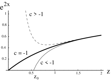
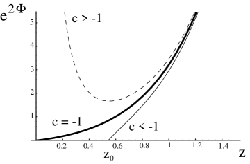
Figure 5: On the left we plot $e^{2x}$, as given by (A.26), for the three ranges of $c$. On the right we represent the corresponding values of $e^{2\Phi}$ for $\tilde{\theta}=\pi/2$ and different values of $c$.

The behavior and interpretation of the solution changes significantly with the value of the integration constant $c$ in (A.26) (see figure 5). On the one hand, $e^{2x}$ tends to one at $z\rightarrow\infty$ for any $c$, while for $z\rightarrow 0$, $e^{2x}$ diverges for $c>-1$ and vanishes for $c=-1$. In contrast, when $c<-1$, $e^{2x}$ vanishes at some finite value $z_{0}>0$ and becomes negative for $z<z_{0}$. We would like to argue, following closely a similar analysis in ref. [6], that this last $c<-1$ case is the one that has a cleaner physical interpretation. With this purpose, let us look at the form of the dilaton (A.31) for $\tilde{\theta}=\pi/2$. As shown in figure 5, the dilaton either diverges or vanishes at some some value of $z$, making the ten-dimensional metric (A.29) singular at that point (see also (2.1)). According to the criteria of ref. [3] a singularity is “good” if the norm of the time-like Killing vector field in the Einstein frame is decreasing as one approaches the singularity. This norm is given by the $G_{tt}$ component of the Einstein frame metric, which in our case is simply $e^{\Phi/2}$. Looking at the behavior of the dilaton in figure 5 we immediately conclude that the singularity is good only for $c<-1$, as claimed in the main text.

A.1.3 UV and IR limits

Let us now discuss in detail the behavior of the solution in the UV and IR regions. The UV limit of the metric and dilaton is obtained by taking $z\rightarrow\infty$. In this limit one readily verifies that $e^{2x},\Sigma\rightarrow 1$ and, therefore, the metric (A.29) and the dilaton (A.31) become:

$$ds^{2}\,\approx\,e^{\Phi}\,\Bigg{[}dx_{1,1}^{2}+{z\over m^{2}}\left(d\theta_{1}^{2}+\sin^{2}\theta_{1}\,d\phi_{1}^{2}+d\theta_{2}^{2}+\sin^{2}\theta_{2}\,d\phi_{2}^{2}\right)+{dz^{2}\over m^{2}}\,+\qquad\qquad\qquad\qquad$$

$$\qquad\qquad+{1\over m^{2}}\,\Big{[}\,\,d\tilde{\theta}^{2}\,+\,\sin^{2}\tilde{\theta}\,d\tilde{\phi}_{2}^{2}\,+\,\cos^{2}\tilde{\theta}\left(d\tilde{\phi}_{1}-\cos\theta_{1}d\phi_{1}-\cos\theta_{2}d\phi_{2}\right)^{2}\,\Big{]}\Bigg{]}\,\,,$$

$$e^{2\Phi}\,\approx\,e^{2z}\,\,.$$ (A.36)

This form of the metric and dilaton do indeed correspond to a stack of D5-branes with worldvolume $\mathbb{R}^{1,1}\times S^{2}\times S^{2}$, with the appropriate twisting.

Let us next consider the IR limit. As explained in the previous subsection, the IR behavior of the solution strongly depends on the value of the integration constant $c$. From now on we will concentrate on the case $c<-1$. In this case the space ends at $z=z_{0}$, where $z_{0}$ is such that $e^{2x(z)}$ vanishes and is given by the solution of the equation:

$$e^{-2z_{0}}\,=\,-{1\over c}\,\big{[}\,1\,-\,2z_{0}\,+2z_{0}^{2}\,\big{]}\,\,.$$ (A.37)

Near $z=z_{0}$ the function $e^{2x(z)}$ can be expanded as:

$$e^{2z}\,\approx 2(z-z_{0})\,\,.$$ (A.38)

Notice that, in the plane of the ten-dimensional coordinates $(\rho,\sigma)$, $z=z_{0}$ is not a point but rather the line $(\sigma=0,0\leq\rho\leq e^{z_{0}})$, parametrized by the angle $\tilde{\theta}$ (see (A.33)). The dilaton becomes singular for $z=z_{0}$ and $\tilde{\theta}={\pi\over 2}$. Let us expand the solution near this point. For this purpose we introduce new coordinates $(\zeta,\psi)$, defined as:

$$\sqrt{2(z-z_{0})}\,=\,\sqrt{\zeta}\,\sin\Big{(}{\psi\over 2}\Big{)}\,\,,\qquad\qquad{\pi\over 2}\,-\,\tilde{\theta}\,=\,\sqrt{\zeta}\,\cos\Big{(}{\psi\over 2}\Big{)}\,\,.$$ (A.39)

Notice that in these coordinates the singularity is just located at $\zeta=0$. One can check that, at first order in $\zeta$:

$$\Sigma\,\approx\,{\sqrt{\zeta}\over\sin\big{(}{\psi\over 2}\big{)}}\,\,.$$ (A.40)

Using this result one can readily verify that, near the singularity, the metric and dilaton can be written as:

$$ds^{2}\,\approx\,e^{\Phi}\,\Bigg{[}dx_{1,1}^{2}+{z_{0}\over m^{2}}\left(d\theta_{1}^{2}+\sin^{2}\theta_{1}\,d\phi_{1}^{2}+d\theta_{2}^{2}+\sin^{2}\theta_{2}\,d\phi_{2}^{2}\right)+\qquad\qquad\qquad\qquad$$

$$+{1\over 4m^{2}\zeta}\,\Big{[}d\zeta^{2}\,+\,\zeta^{2}\,d\psi^{2}\,+\,\zeta^{2}\,\sin^{2}\psi\,\left(d\tilde{\phi}_{1}-\cos\theta_{1}d\phi_{1}-\cos\theta_{2}d\phi_{2}\right)^{2}+\,d\tilde{\phi}_{2}^{2}\,\Big{]}\Bigg{]}\,\,,$$

$$e^{2\Phi}\,\approx e^{2z_{0}}\,\zeta\,\,,$$ (A.41)

which is precisely the form of the metric and dilaton for a stack of D5-branes located at $\zeta=0$ (or $z=z_{0}$, $\tilde{\theta}=\pi/2$) and smeared on a circle along the $\tilde{\phi}_{2}$ direction (notice that the space transverse to the branes is (fibered) $\mathbb{R}^{3}\times S^{1}$ and $1/\zeta$ is a harmonic function in this space). This result implies that our solutions can be interpreted as the gravity duals of a particular slice of the Coulomb branch of the ${\cal N}=(2,2)$ SYM theory, namely the one that is generated when the wrapped D5-branes are moved along an angular direction which is transverse both to the $CY_{3}$ and the D5-brane worldvolume.

A.2 Fivebranes wrapping a co-associative four-cycle

Let us now try to find a solution of $SO(4)$ seven-dimensional gauged supergravity corresponding to a fivebrane wrapping a co-associative four-cycle as described in [38]. The ansatz for the 7d metric is:

$$ds^{2}=e^{2f}\left(dx_{1,1}^{2}+dr^{2}\right)+{e^{2g}\over m^{2}}\,d\Omega_{4}^{2}\,,$$ (A.42)

where $d\Omega_{4}^{2}$ is the metric of a four-sphere, which was defined in (3.1) in terms of the $SU(2)$ left-invariant one-forms $\omega^{i}$ and the coordinate $\xi$. We shall then consider the following one-form frame:

$$e^{x^{\mu}}=e^{f}\,dx^{\mu}\;,\qquad e^{r}=e^{f}\,dr\;,\qquad e^{4}={e^{g}\over m}\,{2\over 1+\xi^{2}}\,d\xi\,,$$

$$e^{i}={e^{g}\over m}\,{\xi\over 1+\xi^{2}}\,\omega^{i}\;,\quad(i=1,2,3)\,.$$ (A.43)

Following [38], in order to implement the topological twist, we shall take the one-form gauge field to be proportional to the anti-self dual part of the spin connection along the four-sphere, namely:

$$A^{12}={1\over 2m}\,{\xi^{2}\over 1+\xi^{2}}\,\,\omega^{1}\,,\qquad A^{13}=-{1\over 2m}\,{\xi^{2}\over 1+\xi^{2}}\,\,\omega^{2}\,,\qquad A^{23}=-{1\over 2m}\,{\xi^{2}\over 1+\xi^{2}}\,\,\omega^{3}\,.$$ (A.44)

Moreover, we will take the following ansatz for the scalars:

$$V_{ij}=e^{\lambda\over 8}\,(e^{x\over 2},e^{x\over 2},e^{x\over 2},e^{-{3\over 2}x})\,,$$ (A.45)

where $\lambda$ and $x$ are fields that depend only on the radial coordinate $r$. Hence, $T_{ij}$ is given by:

$$T_{ij}=V^{-1}_{ik}\,V^{-1}_{kj}=e^{-{\lambda\over 4}}\,(e^{-x},e^{-x},e^{-x},e^{3x})\,,$$ (A.46)

whereas $P_{\mu\;ij}$ and $Q_{\mu\;ij}$ take the form:

$$P_{\mu\;ij}=\delta_{\mu\,r}\left[{\lambda^{\prime}\over 8}(1,1,1,1)+{x^{\prime}\over 2}(1,1,1,-3)\right]\,,\qquad\qquad Q_{\mu\;ij}=2m\,A^{ij}_{\mu}\,,$$ (A.47)

where the prime denotes derivative with respect to $r$.

A.2.1 BPS equations

The SUSY variations will result in a system of first-order differential equations upon imposing the following set of four independent projections:

$$\gamma_{1234}\,\epsilon=\epsilon\,,\quad\gamma_{12}\,\epsilon=\Gamma_{23}\,\epsilon\,,\quad\gamma_{13}\,\epsilon=\Gamma_{31}\,\epsilon\,,\quad\gamma_{r}\,\epsilon=\epsilon\,,$$ (A.48)

where the indices of the $\gamma$’s refer to the frame (A.43). From the analysis of the supersymmetry variations of the gravitino and dilatino one readily concludes that, also in this case, one can take $\lambda=4f$. The system of first-order differential equations one arrives at is:

$$h^{\prime}+{3m\over 2}\,e^{-2h+x}=0\,,$$

$$x^{\prime}+{m\over 2}\left(e^{-x}-e^{3x}\right)-m\,e^{-2h+x}=0\,,$$

$$f^{\prime}+{m\over 10}\left(3e^{-x}+e^{3x}\right)-{3m\over 5}\,e^{-2h+x}=0\,,$$ (A.49)

where, as in (A.21), we have defined $h=g-f$. After defining a new radial variable $z=e^{2h}$, one gets:

$$\dot{x}+{1\over 3}\sinh{2x}+{1\over 3z}=0\,,$$

$$\dot{f}-{1\over 30}\left(3e^{-2x}+e^{2x}\right)+{1\over 5z}=0\,,$$ (A.50)

with the dot denoting derivative with respect to $z$. Moreover, it follows from the first equation in (A.49) that the two radial variables $z$ and $r$ are related as:

$$dz=-3m\,e^{x}\,dr\,.$$ (A.51)

It turns out that the system (A.50) can be solved analytically in terms of Bessel functions. First, for $x(z)$ one gets the following family of solutions:

$$e^{2x}={I_{-{5\over 6}}\,({z\over 3})+c\,I_{{5\over 6}}\,({z\over 3})\over I_{1\over 6}\,({z\over 3})+c\,I_{-{1\over 6}}\,({z\over 3})}\,,$$ (A.52)

where $c$ is an integration constant. Note that $x(z)$ is just the function defined in (3.22). Then, plugging this solution into the second equation in (A.50) it yields:

$$e^{f}=\left[\left(I_{-{5\over 6}}\left({z\over 3}\right)+c\,I_{{5\over 6}}\left({z\over 3}\right)\right)^{3}\left(I_{1\over 6}\,({z\over 3})+c\,I_{-{1\over 6}}\,({z\over 3})\right)z^{2\over 3}\right]^{1\over 10}\,.\,$$ (A.53)

where $c$ is the same real constant as in (A.52).

A.2.2 Ten-dimensional solution

Let us now uplift the solution just found to ten-dimensions. In this case it is more useful to use the following parametrization of the $\mu^{i}$’s:

$$\mu^{1}=\sin{\psi}\,\sin{\theta}\,\cos{\phi}\,,\quad\mu^{2}=\sin{\psi}\,\sin{\theta}\,\sin{\phi}\,,$$

$$\mu^{3}=\sin{\psi}\,\cos{\theta}\,,\quad\mu^{4}=\cos{\psi}\,,$$ (A.54)

with $0\leq\theta,\psi\leq\pi\,$, and $0\leq\phi\leq 2\pi\,$. Using these coordinates, the quantities $Y$ and $\Delta$ defined in (A.10) take the form:

$$Y=e^{-4f}\,\,,\qquad\qquad\Delta\,=\,e^{x-f}\,\,\Theta\,\,,$$ (A.55)

where $\Theta$ is defined as:

$$\Theta=e^{-2x}\,\sin^{2}\psi+e^{2x}\,\cos^{2}\psi\,.$$ (A.56)

Let us now write the complete ten-dimensional solution for a D5-brane. After applying an S-duality transformation to the result obtained from (A.8), we get that the dilaton is given by:

$$e^{2\Phi}\,=\,e^{5f+x}\,\,\Theta\,\,,$$ (A.57)

while the string frame metric becomes:

$$ds^{2}=e^{\Phi}\,\Bigg{[}\,dx_{1,1}^{2}+{e^{-2x}\over 9\,m^{2}}\,dz^{2}+{z\over m^{2}}\,d\Omega^{2}_{4}\,+\,{e^{-2x}\over m^{2}}\,d\psi^{2}\,+\,{\sin^{2}\psi\over m^{2}\Theta}\left[(E^{1})^{2}+(E^{2})^{2}\right]\,\Bigg{]}\,,$$ (A.58)

where $E^{1}$ and $E^{2}$ are the one-forms defined in (3.2). The calculation of the RR three-form $F_{3}$ from (A.12) is straightforward but rather tedious. The final result can be compactly written in terms of the two-form potential $C_{2}$ (see (3.7)), which can be recast in terms of two functions $g_{1}$ and $g_{2}$ as in (3.8). The value of these functions is rather simple, namely:

$$g_{1}\,=\,{1\over m^{2}}\,\,\Big{(}\,{\sin\psi\cos\psi\over\Theta}\,e^{2x}\,-\,\psi\,\Big{)}\,\,,\qquad\qquad g_{2}\,=\,{\psi\over m^{2}}\,\,.$$ (A.59)

In order to make contact with the ten-dimensional approach of section 3, let us now define the new set of variables:

$$\sigma\,=\,z^{{2\over 3}}\,e^{{5\over 2}f\,+\,{x\over 2}}\,\sin\psi\,\,,\qquad\qquad\rho\,=\,e^{{5\over 2}f\,-\,{3x\over 2}}\,\cos\psi\,\,.$$ (A.60)

In terms of the dilaton $\Phi$, the above relations can be written as:

$$\sigma\,=\,{z^{{2\over 3}}\,e^{\Phi}\over\sqrt{\Theta}}\,\sin\psi\,\,,\qquad\qquad\rho\,=\,\,{e^{\Phi-2x}\over\sqrt{\Theta}}\,\cos\psi\,\,,$$ (A.61)

where we have taken into account the relation (A.57). By using (see (A.50)):

$${5\over 2}\dot{f}\,+\,{\dot{x}\over 2}\,=\,{e^{-2x}\over 3}\,-\,{2\over 3z}\,\,,\qquad\qquad{5\over 2}\dot{f}\,-\,{3\dot{x}\over 2}\,=\,{1\over 3}e^{2x}\,\,,$$ (A.62)

one can prove straightforwardly that:

$$d\sigma\,=\,{e^{\Phi}\over\sqrt{\Theta}}\,\,z^{{2\over 3}}\,\Big{[}\,{e^{-2x}\over 3}\sin\psi\,dz\,+\,\cos\psi\,d\psi\,\Big{]}\,\,,$$

$$d\rho\,=\,{e^{\Phi}\over\sqrt{\Theta}}\Big{[}\,{\cos\psi\over 3}\,dz\,-\,\sin\psi\,e^{-2x}\,d\psi\,\Big{]}\,\,.$$ (A.63)

The inverse of this relation is:

$$dz\,=\,{e^{-\Phi}\over\sqrt{\Theta}}\,\,\Big{(}\,3z^{-{2\over 3}}\,\sin\psi\,d\sigma\,+\,3e^{2x}\,\cos\psi\,d\rho\,\Big{)}\,\,,$$

$$d\psi\,=\,{e^{-\Phi}\over\sqrt{\Theta}}\,\,\Big{(}\,z^{-{2\over 3}}\,e^{2x}\,\cos\psi\,d\sigma\,-\,\sin\psi\,d\rho\,\Big{)}\,\,.$$ (A.64)

It is now immediate to verify that the metric (A.58) can be written as in our ten-dimensional ansatz (3.4). Moreover, the gauged supergravity analysis provides a particular highly non-trivial solution of the BPS system (3.15). In order to write this solution entirely in terms of the ten-dimensional variables $\rho$ and $\sigma$, let us notice that, after using (A.52) and (A.53), we get:

$$e^{{5\over 2}f\,+\,{x\over 2}}\,=\,z^{{1\over 6}}\,\Big{|}\,I_{-{5\over 6}}\,({z\over 3})+c\,I_{{5\over 6}}\,({z\over 3})\,\Big{|}\,\,\,,\qquad\qquad e^{{5\over 2}f\,-\,{3x\over 2}}\,=\,z^{{1\over 6}}\,\Big{|}\,I_{{1\over 6}}\,({z\over 3})+c\,I_{-{1\over 6}}\,({z\over 3})\,\Big{|}\,\,\,.$$ (A.65)

Thus, we can rewrite (A.60) as:

$$\sigma\,=\,z^{{5\over 6}}\,\Big{|}\,I_{-{5\over 6}}\,({z\over 3})+c\,I_{{5\over 6}}\,({z\over 3})\,\Big{|}\,\sin\psi\,\,,\qquad\qquad\rho\,=\,z^{{1\over 6}}\,\Big{|}\,I_{{1\over 6}}\,({z\over 3})+c\,I_{-{1\over 6}}\,({z\over 3})\,\Big{|}\,\cos\psi\,\,.$$ (A.66)

After eliminating the angle $\psi$ in (A.66), we get the implicit solution written in (3.21) of the PDE (3.19). Moreover, one can check that, when expressed in terms of the variables $\rho$ and $\sigma$, the dilaton $\Phi$ and the functions $g_{1}$ and $g_{2}$ written in eqs. (A.57) and (A.59) coincide with the ones of (3.23) and (3.25).

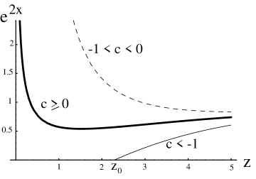
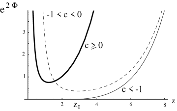
Figure 6: On the left we plot $e^{2x}$ for three ranges of the constant $c$ in (A.52). The plots on the right represent $e^{2\Phi}$, taken from (A.57), for $\psi=0$.

Let us now study the behavior of the solution for the different values of the integration constant $c$ of eqs. (A.52) and (A.53). The different behaviors of the function $e^{2x}$ are plotted in figure 6 for three ranges of $c$. When $c\geq 0$ $e^{2x}$ diverges at $z=0$. On the contrary if $-1<c<0$ the function $e^{2x}$ diverges at some point $\tilde{z}_{0}$ such that $I_{1\over 6}({\tilde{z}_{0}\over 3})+c\,I_{-{1\over 6}}({\tilde{z}_{0}\over 3})=0$, which marks the end of the space. The solution is not well-defined for $c=-1$ since in this case $e^{2x}$ is negative for $z>0$. Finally, when $c<-1$ $e^{2x}$ vanishes at $z=z_{0}$, where $z_{0}$ has been defined in (3.26). The behavior of the dilaton for the three ranges of $c$ is also displayed in figure 6. From this figure we conclude that only when $c<-1$ the $tt$ component of the Einstein frame metric, namely $e^{\Phi/2}$, decreases when we approach the singularity and, thus, only in this $c<-1$ case is the singularity good. Actually, $z=z_{0}$ defines a line of singularities. This fact can be checked by analyzing the form of the dilaton around $z=z_{0}$. Indeed, by using the properties of the modified Bessel functions one can verify that, for $z$ close to $z_{0}$, one has:

$$e^{2x}\,\approx{1\over 3}\,\,(z-z_{0})\,,$$

$$I_{-{5\over 6}}\Big{(}{z\over 3}\Big{)}+c\,I_{{5\over 6}}\Big{(}{z\over 3}\Big{)}\,\approx\,{\gamma\over 3}\,(z-z_{0})\,\,,$$

$$e^{5f}\,\approx\,{z_{0}^{{1\over 3}}\gamma^{2}\over 3\sqrt{3}}\,\,(z-z_{0})^{{3\over 2}}\,\,,$$ (A.67)

where $\gamma$ is a constant (depending on $z_{0}$ and $c$) defined as:

$$\gamma\equiv I_{{1\over 6}}\Big{(}{z_{0}\over 3}\Big{)}+c\,I_{-{1\over 6}}\Big{(}{z_{0}\over 3}\Big{)}\,\,.$$ (A.68)

Using this result in (A.57) one arrives at the following expression of $e^{2\Phi}$ for $z\rightarrow z_{0}$:

$$e^{2\Phi}\,\approx\,{z_{0}^{{1\over 3}}\gamma^{2}\over 3}\,(z-z_{0})\,\Big{[}\,\sin^{2}\psi\,+\,{(z-z_{0})^{2}\over 9}\,\,\cos^{2}\psi\,\Big{]}\,\,,$$ (A.69)

which shows that $e^{2\Phi}\rightarrow 0$ for any value of $\psi$ in the interval $[0,\pi]$. Notice that, in terms of the variables $\sigma$ and $\rho$ of (A.66), the singularities lie in the segment $\sigma=0,|\rho|\leq\rho_{c}$, where $\rho_{c}$ has been defined in (3.27), as claimed at the end of subsection 3.1.

A.2.3 UV and IR limits

We will now discuss the UV and IR limits of the solution found, following the analysis of ref. [12]. First of all, we consider the UV limit of the metric, by taking $z\rightarrow\infty$. In order to take this limit in our solution it is quite useful to recall the asymptotic behavior of the modified Bessel functions, namely:

$$I_{\nu}\Big{(}{z\over 3}\Big{)}\,\approx\sqrt{{3\over 2\pi}}\,\,{e^{{z\over 3}}\over\sqrt{z}}\,\,,\qquad\qquad z\rightarrow\infty\,\,.$$ (A.70)

It follows from this behavior that $e^{2x}\rightarrow 1$ and $\Omega\rightarrow 1$ in the large $z$ limit. Therefore, in the UV the metric and dilaton take the form:

$$ds^{2}\approx\,e^{\Phi}\,\Bigg{[}\,dx^{2}_{1,1}\,+\,{z\over m^{2}}\,d\Omega_{4}^{2}\,+\,{1\over m^{2}}\,\,\Big{[}\,{1\over 9}\,dz^{2}\,+\,d\psi^{2}\,+\,\sin^{2}\psi\,\big{[}\,\big{(}E^{1}\big{)}^{2}\,+\,\big{(}E^{2}\big{)}^{2}\,\big{]}\Big{]}\,\Bigg{]}\,\,,$$

$$e^{2\Phi}\,\approx\,{3\over 2\pi}\,\,{e^{{2z\over 3}}\over z^{{2\over 3}}}\,\,,$$ (A.71)

which, indeed, corresponds to a stack of D5-branes with worldvolume $\mathbb{R}^{1,1}\times S^{4}$.

Let us next explore the IR behavior of our background. We will concentrate on the case in which $c<-1$, which is singular at a point $z=z_{0}$, with $z_{0}$ being defined in (3.26). In order to study the limiting form of the metric and dilaton near the singularity we have to expand all functions around $z=z_{0}$ as in (A.67). If we define a new radial variable $y$ as:

$$y={1\over 3}\,\,(z-z_{0})\,\,,$$ (A.72)

then, the metric and dilaton take the form (for $\psi\not=0,\pi$):

$$ds^{2}\,\approx\,e^{\Phi}\,\Bigg{[}\,dx^{2}_{1,1}\,+\,{z_{0}\over m^{2}}\,d\Omega_{4}^{2}\,+\,{1\over m^{2}\,y}\,\Big{[}\,dy^{2}\,+\,y^{2}\,\big{[}\,\big{(}E^{1}\big{)}^{2}\,+\,\big{(}E^{2}\big{)}^{2}\,\big{]}\,+\,d\psi^{2}\,\Big{]}\,\Bigg{]}\,\,,$$

$$e^{-2\Phi}\,\approx\,\gamma^{2}\,z_{0}^{{1\over 3}}\,y\,\sin^{2}\psi\,\,.$$ (A.73)

This form of the metric indicates that the singularity is generated by a distribution of branes parametrized by the the coordinate $\psi$. As $0\leq\psi\leq\pi$ this distribution has the topology of a segment and can be regarded as a linear distribution of branes which is dual to a slice of the Coulomb branch of the ${\cal N}=(1,1)$ SYM. In order to confirm this interpretation, let us analyze, following ref. [12], the solution near $\psi=0$. With this purpose we introduce new coordinates $r$ and $\alpha$, defined as:

$${1\over 3}\,\,(z-z_{0})\,=\,\sqrt{r}\,\,\sin\Big{(}{\alpha\over 2}\Big{)}\,\,,$$

$$\psi\,=\,\sqrt{r}\,\,\cos\Big{(}{\alpha\over 2}\Big{)}\,\,.$$ (A.74)

In these variables, for small $\psi$, one can check that $\Theta$, as defined in (A.56) is given by:

$$\Theta\,\approx\,{\sqrt{r}\over\sin\big{(}{\alpha\over 2}\big{)}}\,\,.$$ (A.75)

Then, one can check that metric and dilaton are:

$$ds^{2}\,\approx\,e^{\Phi}\,\Bigg{[}\,dx^{2}_{1,1}\,+\,{z_{0}\over m^{2}}\,d\Omega_{4}^{2}\,+\,{1\over 4m^{2}r^{{3\over 2}}\,\sin\big{(}{\alpha\over 2}\big{)}}\,\,\Big{[}\,dr^{2}\,+\,r^{2}\,\Big{(}\,d\alpha^{2}\,+\,\sin^{2}\alpha\,\big{[}\,\big{(}E^{1}\big{)}^{2}\,+\,\big{(}E^{2}\big{)}^{2}\,\big{]}\,\Big{)}\,\Big{]}\,\Bigg{]}\,\,,$$

$$e^{-2\Phi}\,\approx\,\gamma^{2}\,z_{0}^{{1\over 3}}\,r^{{3\over 2}}\,\sin\big{(}{\alpha\over 2}\big{)}\,\,,$$ (A.76)

which, as argued in [12], is consistent with the interpretation of the solution given above since $1/r^{{3\over 2}}\,\sin\big{(}{\alpha\over 2}\big{)}$ is a harmonic function in $\mathbb{R}^{4}$.

Appendix B Additional fivebrane solutions

In this appendix we will show that there exist solutions of the unflavored BPS systems (2.11) and (3.15) that are different from the ones obtained in gauged supergravity. We will find these solutions directly by adopting an ansatz in which the two ten-dimensional variables $\rho$ and $\sigma$ are separated. We will consider first the BPS system for the background with four supersymmetries and, subsequently, we will attack the system of BPS equations corresponding to the preservation of two SUSYs.

B.1 Backgrounds with four supersymmetries

Let us try to solve the BPS system (2.11) by means of the ansatz:

$$g\,=\,g(\sigma)\,\,,\qquad\qquad\Phi=\Phi(\rho)\,\,,$$ (B.1)

Notice that the third equation in (2.11) is automatically solved by the ansatz. As the last equation is a consequence of the other three equations, we only need to solve the first two equations in (2.11). By integrating the second equation in (2.11) over $\sigma$, we get:

$$z^{3}\,=\,{3\sigma^{2}\over 2}\,\,e^{-2\Phi}\,+\,f(\rho)\,\,,$$ (B.2)

where $f(\rho)$ is an unknown function to be determined. Moreover, by integrating the first equation in (2.11) we get:

$$z\,=\,B(\sigma)\,+\,m^{2}\,g(\sigma)\,\log(\rho)\,\,,$$ (B.3)

where $B(\sigma)$ is a function to be determined. By combining these last two equations, we get:

$${3\sigma^{2}\over 2}\,\,e^{-2\Phi}\,+\,f(\rho)\,=\,\Big{(}\,B(\sigma)\,+\,m^{2}\,g(\sigma)\,\log(\rho)\,\Big{)}^{3}\,\,.$$ (B.4)

By comparing the $\sigma$ dependence of both sides of (B.4) one concludes straightforwardly that the four functions $B^{3}(\sigma)$, $B^{2}(\sigma)\,g(\sigma)$, $B(\sigma)\,g^{2}(\sigma)$ and $g^{3}(\sigma)$ must be polynomials in $\sigma$ of second degree. This, in turn, is only possible if $B(\sigma)$ and $g(\sigma)$ are proportional to each other. Let us write:

$$m^{2}\,g(\sigma)\,=\,\kappa B(\sigma)\,\,,\qquad\qquad B^{3}(\sigma)\,=\,b_{2}\,\sigma^{2}\,+\,b_{1}\,\sigma\,+\,b_{0}\,\,,$$ (B.5)

where $\kappa$, $b_{0}$, $b_{1}$ and $b_{2}$ are constants. Actually, the absence of linear terms in $\sigma$ on the left-hand-side of (B.4) implies that $b_{1}=0$. Thus, we write:

$$B(\sigma)\,=\,(\,b_{2}\,\sigma^{2}\,+\,b_{0}\,)^{{1\over 3}}\,\,.$$ (B.6)

By using this expression of $B(\sigma)$ in (B.4) one easily gets the form of the dilaton $\Phi$ and the integration function $f$, namely:

$$e^{2\Phi(\rho)}\,=\,{3\over 2b_{2}}\,\,{1\over\big{(}\,1\,+\,\kappa\,\log(\rho)\,\big{)}^{3}}\,\,,\qquad\qquad f(\rho)\,=\,b_{0}\,\big{(}\,1\,+\,\kappa\,\log(\rho)\,\big{)}^{3}\,\,.$$ (B.7)

The corresponding expressions for $z$ and $g$ are:

$$z\,=\,\big{(}\,b_{2}\,\sigma^{2}\,+\,b_{0}\,\big{)}^{{1\over 3}}\,\big{(}\,1\,+\,\kappa\,\log(\rho)\,\big{)}\,\,,\qquad\qquad g\,=\,{\kappa\over m^{2}}\,\,\big{(}\,b_{2}\,\sigma^{2}\,+\,b_{0}\,\big{)}^{{1\over 3}}\,\,.$$ (B.8)

Let us now change from the radial variable $\sigma$ to a new one $r$, defined as:

$$r^{2}\,=\,{6\over m^{2}}\,\,\sqrt{{3\over 2b_{2}}}\,\big{(}\,b_{2}\,\sigma^{2}\,+\,b_{0}\,\big{)}^{{1\over 3}}\,\,,$$ (B.9)

and let us introduce a new mass parameter $\mu$, which has the form:

$$\mu^{2}\,=\,\sqrt{{3\over 2b_{2}}}\,\,m^{2}\,\,.$$ (B.10)

Then, after rescaling the Minkowski coordinates in the appropriate way and by redefining the $\rho$ coordinate as $\rho/\mu\rightarrow\rho$, the metric takes the form:

$$ds^{2}\,=\,{dx^{2}_{1,1}\over\big{(}\,1\,+\,\kappa\,\log(\mu\rho)\,\big{)}^{{3\over 2}}}\,+\,\big{(}\,1\,+\,\kappa\,\log(\mu\rho)\,\big{)}^{{3\over 2}}\,\big{(}\,d\rho^{2}\,+\,\rho^{2}\,d\chi^{2}\,\big{)}\,+\,$$

$$\qquad\qquad\qquad\qquad\qquad\qquad+\,\big{(}\,1\,+\,\kappa\,\log(\mu\rho)\,\big{)}^{-{1\over 2}}\,ds^{2}_{6}\,\,,$$ (B.11)

where $ds^{2}_{6}$ is the metric of the conifold with a blown up four-cycle (the regularized conifold):

$$ds^{2}_{6}\,=\,{r^{2}\over 6}\,\,\Big{(}\,d\theta_{1}^{2}\,+\,\sin^{2}\theta_{1}\,d\phi_{1}^{2}\,+\,d\theta_{2}^{2}\,+\,\sin^{2}\theta_{2}\,d\phi_{2}^{2}\,\Big{)}\,+\,{dr^{2}\over 1\,-\,{a^{6}\over r^{6}}}\,+\,$$

$$\qquad\qquad\qquad\qquad+{r^{2}\over 9}\,\,\Big{(}1\,-\,{a^{6}\over r^{6}}\Big{)}\,\Big{(}\,d\psi\,+\,\cos\theta_{1}d\phi_{1}\,+\,\cos\theta_{2}d\phi_{2}\,\Big{)}^{2}\,\,,$$ (B.12)

with the constant $a$ being:

$$a\,=\,{(b_{0})^{{1\over 6}}\over m}\,\,\Big{(}{54\over b_{2}}\Big{)}^{{1\over 4}}\,\,.$$ (B.13)

Notice that the variables $r$ and $\rho$ in (B.11) and (B.12) are dimensionful. Moreover, the dilaton and $g$ are given by:

$$e^{\Phi}\,=\,{\mu^{2}\over m^{2}}\,\,{1\over\big{(}\,1\,+\,\kappa\,\log(\mu\rho)\,\big{)}^{{3\over 2}}}\,\,,\qquad\qquad g\,=\,\kappa\,{\mu^{2}\over m^{2}}\,{r^{2}\over 6}\,\,.$$ (B.14)

The RR field strength $F_{3}$ that corresponds to the function $g$ written above is:

$$F_{3}\,=\,\kappa\,{\mu^{2}\over m^{2}}\,\Big{[}\,{r^{2}\over 6}\,\Big{(}\sin\theta_{1}d\theta_{1}\wedge d\phi_{1}\,+\,\sin\theta_{2}d\theta_{2}\wedge d\phi_{2}\Big{)}\,+\,$$

$$\qquad\qquad\qquad+{r\over 3}\,\Big{(}d\psi\,+\,\cos\theta_{1}d\phi_{1}\,+\,\cos\theta_{2}d\phi_{2}\,\Big{)}\wedge dr\,\Big{]}\,\wedge d\chi\,\,.$$ (B.15)

Let us rewrite this expression for $F_{3}$ in a more compact form. With this purpose, let us introduce the following vielbein basis for the conifold metric:

$$E^{1}\,=\,{r\over\sqrt{6}}\,d\theta_{1}\,\,,\qquad\qquad\qquad E^{2}\,=\,{r\over\sqrt{6}}\,\sin\theta_{1}\,d\phi_{1}\,\,,$$

$$E^{3}\,=\,{r\over\sqrt{6}}\,d\theta_{2}\,\,,\qquad\qquad\qquad E^{4}\,=\,{r\over\sqrt{6}}\,\sin\theta_{2}\,d\phi_{2}\,\,,$$

$$E^{5}\,=\,{r\over 3}\,\Big{(}1\,-\,{a^{6}\over r^{6}}\Big{)}^{{1\over 2}}\,\Big{(}d\psi\,+\,\cos\theta_{1}d\phi_{1}\,+\,\cos\theta_{2}d\phi_{2}\,\Big{)}\,\,,$$

$$E^{6}\,=\,{dr\over\Big{(}1\,-\,{a^{6}\over r^{6}}\Big{)}^{{1\over 2}}}\,\,.$$ (B.16)

In terms of this basis the Kähler form of the conifold takes the form:

$$J\,=\,E^{1}\wedge E^{2}\,+\,E^{3}\wedge E^{4}\,+\,E^{5}\wedge E^{6}\,\,,$$ (B.17)

and the RR three form $F_{3}$ is just given by:

$$F_{3}\,=\,\kappa\,{\mu^{2}\over m^{2}}\,J\wedge d\chi\,\,.$$ (B.18)

B.2 Backgrounds with two supersymmetries

In this subsection we want to obtain new solutions of the first-order BPS system (3.15), different from the one we got from gauged supergravity. We have been able to find two different ansätze to solve this system that we detail in the next two subsections.

B.2.1 First ansatz

As a first possibility for getting new solutions of the BPS system (3.15), let us adopt the following ansatz for $z$, $g_{1,2}$ and $\Phi$:

$$z\,=\,z(\sigma)\,\,,\qquad g_{1}(\rho)\,=\,-g_{2}(\rho)\,\,,\qquad\Phi\,=\,\Phi(\sigma)\,\,.$$ (B.19)

Notice that ${\rm 2}^{\rm nd}$, ${\rm 4}^{\rm th}$ and ${\rm 5}^{\rm th}$ equations in (3.15) are automatically solved by the ansatz. Moreover, the ${\rm 6}^{\rm th}$ equation in (3.15), namely:

$$g_{2}^{\prime}\,=\,-{\sigma\over m^{2}z^{{2\over 3}}}\,e^{-2\Phi}\,\,,$$ (B.20)

is such that the left-hand side only depends on $\rho$, whereas the right-hand side depends of $\sigma$. Separating variables, we get:

$$g_{2}^{\prime}\,=\,c_{1}\,\,,\qquad\qquad\sigma\,e^{-2\Phi}\,=\,-m^{2}c_{1}\,z^{{2\over 3}}\,\,,$$ (B.21)

where $c_{1}$ is a constant. The equation for $g_{2}$ can be immediately integrated, namely:

$$g_{2}\,=\,c_{1}+c_{2}\rho\,\,,$$ (B.22)

where $c_{2}$ is a new constant. Furthermore, using the third equation in the BPS system (3.15) we can obtain the following equation for $z(\sigma)$:

$$z^{{2\over 3}}\,\dot{z}\,=\,-3m^{2}\,c_{1}\,\,,$$ (B.23)

which can also be readily integrated. It is also easy to get the expression of the dilaton. Let us write this solution in terms of new constants $\lambda_{1,2,3}$ defined as $\lambda_{1,2}=-5m^{2}c_{1,2}$ and $\lambda_{3}=5c_{3}$. Then, one has:

$$g_{1}=-g_{2}\,=\,{1\over 5m^{2}}\,\big{(}\,\lambda_{1}\,\rho+\lambda_{2}\,\big{)}\,\,,$$

$$z=\big{[}\,\lambda_{3}\,+\,\lambda_{1}\sigma\,\big{]}^{{3\over 5}}\,\,,\qquad\qquad e^{2\Phi}\,=\,{5\sigma\over\lambda_{1}}\,\big{[}\,\lambda_{3}\,+\,\lambda_{1}\sigma\,\big{]}^{-{2\over 5}}\,\,.$$ (B.24)

It is now convenient to define the function $H(\sigma)$ as:

$$H(\sigma)\,=\,\sqrt{\lambda_{1}\over 5\sigma}\,\,\big{[}\,\lambda_{3}\,+\,\lambda_{1}\sigma\,\big{]}^{{1\over 5}}\,\,.$$ (B.25)

Then, $z$ and $\Phi$ can be rewritten as:

$$z\,=\,\Big{(}{5\sigma\over\lambda_{1}}\Big{)}^{{3\over 2}}\,\Big{[}\,H(\sigma)\,\Big{]}^{3}\,\,,\qquad\qquad e^{\Phi}\,=\,\Big{[}\,H(\sigma)\,\Big{]}^{-1}\,\,,$$ (B.26)

and the metric takes the form:

$$ds^{2}_{10}\,=\,H^{-1}\,dx^{2}_{1,1}\,+\,{1\over m^{2}}\,\Big{(}{5\sigma\over\lambda_{1}}\Big{)}^{{3\over 2}}\,H^{2}\,d\Omega^{2}_{4}\,+\,$$

$$\qquad\qquad+\,{1\over m^{2}}\,\Big{(}{\lambda_{1}\over 5\sigma}\Big{)}^{2}\,\,H^{-3}\,\Big{[}\,d\sigma^{2}\,+\,\sigma^{2}\,\big{(}\,(E^{1})^{2}+(E^{2})^{2}\,\big{)}\,\Big{]}\,+\,{H\over m^{2}}\,(d\rho)^{2}\,\,.$$ (B.27)

Notice that, by plugging the solution for $g_{1}$ and $g_{2}$ into the expression (3.10) of $F_{3}$, we get:

$$F_{3}\,=\,{\lambda_{1}\over 5m^{2}}\,\Big{[}\,E^{1}\wedge E^{2}\,-\,{\cal S}^{\xi}\wedge{\cal S}^{3}\,-\,{\cal S}^{1}\wedge{\cal S}^{2}\,\Big{]}\wedge d\rho\,\,.$$ (B.28)

Let us now rewrite this solution by means of a change of the radial variable: we will change from $\sigma$ to a new variable $r$, related to the former as:

$$r\,=\,{2\sqrt{5}\over 3}\,\lambda_{1}^{{3\over 10}}\,\sigma^{{3\over 10}}\,\,\Big{(}\,1\,+\,{\lambda_{3}\over\lambda_{1}\,\sigma}\,\Big{)}^{{3\over 10}}\,\,.$$ (B.29)

Moreover, instead of the constant $\lambda_{3}$, we will use the constant $l$, defined as:

$$l\,=\,{2\sqrt{5}\over 3}\,\lambda_{3}^{{3\over 10}}\,\,.$$ (B.30)

From these definitions one can check that:

$$1\,-\,{l^{{10\over 3}}\over r^{{10\over 3}}}\,=\,\Big{(}\,1\,+\,{\lambda_{3}\over\lambda_{1}\,\sigma}\,\Big{)}^{-1}\,\,,\qquad\qquad{dr\over r}\,=\,{3\over 10}\,\,\Big{(}\,1\,+\,{\lambda_{3}\over\lambda_{1}\,\sigma}\,\Big{)}^{-1}\,{d\sigma\over\sigma}\,\,.$$ (B.31)

Moreover, after a convenient rescaling of the Minkowski coordinates, the metric and dilaton take the form:

$$ds^{2}_{10}\,=\,e^{2k}\,\Bigg{[}\,dx^{2}_{1,1}\,+\,\Big{(}\,1\,-\,{l^{{10\over 3}}\over r^{{10\over 3}}}\,\Big{)}^{-1}\,\,(dr)^{2}\,+\,{9\over 20}\,r^{2}\,d\Omega_{4}^{2}\,+\,$$

$$\qquad\qquad\qquad\qquad+\,{9\over 100}\,r^{2}\,\,\Big{(}\,1\,-\,{l^{{10\over 3}}\over r^{{10\over 3}}}\,\Big{)}\,\Big{[}\,(E^{1})^{2}\,+\,(E^{2})^{2}\Big{]}\,\,\Bigg{]}\,+\,{e^{-2k}\over m^{4}}\,\,\big{(}d\rho\big{)}^{2}\,\,,$$

$$e^{2\Phi}\,=\,m^{4}\,e^{4k}\,\,,$$ (B.32)

where $k$ is defined as:

$$e^{2k}\,=\,{3\over 2\lambda_{1}m^{2}}\,\,r\,\,\Big{(}\,1\,-\,{l^{{10\over 3}}\over r^{{10\over 3}}}\,\Big{)}^{{1\over 2}}\,\,.$$ (B.33)

In order to identify this background let us perform a T-duality transformation along the coordinate $\rho$ (shifting $\rho$ is an isometry of the background (B.32)). According to the T-duality rules in [45], one should perform the changes:

$$g_{\rho\rho}\,\rightarrow{1\over g_{\rho\rho}}\,\,,\qquad\qquad e^{2\Phi}\rightarrow{e^{2\Phi}\over g_{\rho\rho}}\,\,.$$ (B.34)

Also the RR three-form $F_{3}$ is converted into an RR two-form $F_{2}$. The resulting type IIA background is:

$$ds^{2}_{10}\,=\,e^{2k}\,\Bigg{[}\,dx^{2}_{1,2}\,+\,\Big{(}\,1\,-\,{l^{{10\over 3}}\over r^{{10\over 3}}}\,\Big{)}^{-1}\,\,(dr)^{2}\,+\,{9\over 20}\,r^{2}\,d\Omega_{4}^{2}\,+\,$$

$$\qquad\qquad\qquad\qquad\qquad\qquad+\,{9\over 100}\,r^{2}\,\,\Big{(}\,1\,-\,{l^{{10\over 3}}\over r^{{10\over 3}}}\,\Big{)}\,\Big{[}\,(E^{1})^{2}\,+\,(E^{2})^{2}\Big{]}\,\,\Bigg{]}\,\,,$$

$$e^{2\Phi}\,=\,m^{8}\,e^{6k}\,=\,\Bigg{(}{3m^{{2\over 3}}\over 2\lambda_{1}}\Bigg{)}^{3}\,r^{3}\,\,\Big{(}\,1\,-\,{l^{{10\over 3}}\over r^{{10\over 3}}}\,\Big{)}^{{3\over 2}}\,\,,$$

$$F_{2}\,=\,{\lambda_{1}\over 5m^{2}}\,\Big{[}\,E^{1}\wedge E^{2}\,-\,{\cal S}^{\xi}\wedge{\cal S}^{3}\,-\,{\cal S}^{1}\wedge{\cal S}^{2}\,\Big{]}\,\,.$$ (B.35)

This solution corresponds to a D6-brane wrapped along a four-cycle of a $G_{2}$-cone, which is an analogue in the type IIA theory of the solution found in [8]-[10].

B.2.2 Second ansatz

As a second ansatz, let us now try to find solutions of (3.15) in which the functions $g_{1}$ and $g_{2}$ are proportional to each other. Let us write $g_{1}=\alpha g_{2}$, with $\alpha$ being a constant and let us separate variables as:

$$g_{1}=\alpha g_{2}\,=\,\alpha R(\rho)\,S(\sigma)\,\,,\qquad\qquad z\,=\,z_{1}(\rho)\,z_{2}(\sigma)\,\,.$$ (B.36)

From the ${\rm 5}^{\rm th}$ equation in the BPS system, we get that $S(\sigma)$ satisfies the equation:

$${\dot{S}\over S}\,=\,{1+\alpha\over\sigma}\,\,,$$ (B.37)

which can be immediately integrated as:

$$S(\sigma)\,=\,c_{1}\,\sigma^{1+\alpha}\,\,.$$ (B.38)

By substituting the ansatz in the ${\rm 4}^{\rm th}$ equation of (3.15), using the result just found for $S(\sigma)$ and separating variables, we arrive at:

$${1\over R}\,{z_{1}^{\prime}\over z_{1}^{{2\over 3}}}\,=\,3(1+\alpha)m^{2}\,c_{1}\,\sigma^{\alpha}\,z_{2}^{-{1\over 3}}\,=\,c_{2}\,\,,$$ (B.39)

where $c_{2}$ is a new constant. From this equation we can immediately get $z_{2}(\sigma)$, namely:

$$z_{2}\,=\,\Bigg{[}{3(1+\alpha)m^{2}\,c_{1}\over c_{2}}\Bigg{]}^{3}\,\,\sigma^{3\alpha}\,\,,$$ (B.40)

as well as an equation for $z_{1}(\rho)$ and $R(\rho)$, namely:

$$z_{1}^{-{2\over 3}}\,z_{1}^{\prime}\,=\,c_{2}\,R\,\,.$$ (B.41)

Let us now combine the ${\rm 3}^{\rm rd}$ and ${\rm 6}^{\rm th}$ equations in (3.15) to give:

$${\dot{z}\over g_{2}^{\prime}}\,=\,-{3m^{2}\over z^{{2\over 3}}}\,\,.$$ (B.42)

Using the results just found for $z_{2}(\sigma)$ and $S(\sigma)$ (eqs. (B.40) and (B.38)) and separating variables we get:

$${z_{1}^{{5\over 3}}\over R^{\prime}}\,=\,-{m^{2}c_{1}\over\alpha}\,\,{\sigma^{2+\alpha}\over z_{2}^{{5\over 3}}}\,=\,c_{3}\,\,,$$ (B.43)

where $c_{3}$ is a new constant. The consistency of the $\sigma$-dependent part of equation (B.43) with (B.40) fixes the value of $\alpha$ and relates the constant $c_{3}$ with the other constants $c_{1}$ and $c_{2}$, namely:

$$\alpha={1\over 2}\,\,,\qquad\qquad c_{3}\,=\,-2m^{2}c_{1}\,\,\Big{(}{2c_{2}\over 9m^{2}c_{1}}\Big{)}^{5}\,\,.$$ (B.44)

On the other hand, the $\rho$-dependent part of (B.43), gives rise to the following relation between $z_{1}$ and $R$:

$$z_{1}^{{5\over 3}}\,=\,c_{3}\,R^{\prime}\,\,.$$ (B.45)

By combining (B.41) and (B.45) one can get $z_{1}(\rho)$ in terms of $R(\rho)$, namely:

$$z_{1}(\rho)\,=\,\sqrt{c_{2}\,c_{3}\,R(\rho)^{2}\,+\,c_{4}}\,\,,$$ (B.46)

with $c_{4}$ being a new constant of integration. Moreover, $R(\rho)$ can be obtained as the solution of the equation:

$$R^{\prime}(\rho)\,=\,{1\over c_{3}}\,\Big{[}\,c_{2}\,c_{3}R(\rho)^{2}\,+\,c_{4}\,\Big{]}^{{5\over 6}}\,\,.$$ (B.47)

In order to rewrite this solution, let us define new constants $\lambda$ and $\kappa$ as:

$$\lambda^{2}\,=\,-c_{2}\,c_{3}\,\,,\qquad\qquad\kappa\,=\,{9m^{2}c_{1}\over 2c_{2}}\,\,.$$ (B.48)

The constants $c_{1,2,3}$ can be written in terms of $\lambda$ and $\kappa$ as:

$$c_{1}\,=\,{\lambda\over 3m^{2}}\,\kappa^{3}\,\,,\qquad\qquad c_{2}\,=\,{3\over 2}\,\lambda\kappa^{2}\,\,,\qquad\qquad c_{3}\,=\,-{2\lambda\over 3\kappa^{2}}\,\,.$$ (B.49)

In terms of these new constants $\kappa$ and $\lambda$, the different functions of the ansatz take the form:

$$z\,=\,\kappa^{3}\,\Big{[}\,c_{4}-\lambda^{2}\,R^{2}(\rho)\,\Big{]}^{{1\over 2}}\,\sigma^{{3\over 2}}\,\,,$$

$$g_{1}\,=\,{1\over 2}\,g_{2}\,=\,{\kappa^{3}\,\lambda\over 6m^{2}}\,R(\rho)\,\sigma^{{3\over 2}}\,\,,$$

$$e^{-2\Phi}\,=\,{\kappa^{7}\over 2}\,\,\Big{[}\,c_{4}\,-\,\lambda^{2}\,R(\rho)^{2}\,\Big{]}^{{7\over 6}}\,\,\sigma^{{3\over 2}}\,\,,$$ (B.50)

with $R(\rho)$ satisfying:

$$\lambda\,R^{\prime}(\rho)\,=\,-{3\kappa^{2}\over 2}\,\,\Big{[}\,c_{4}-\lambda^{2}\,R^{2}(\rho)\,\Big{]}^{{5\over 6}}\,\,.$$ (B.51)

In order to write the background obtained in a more convenient way, let us change from the $\rho$ coordinate to a new coordinate $r$, defined as:

$$r\,=\,{R(\rho)\over\sqrt{c_{4}}}\,\,.$$ (B.52)

Moreover, we will redefine again the integration constants and we will introduce new constants $a$ and $b$, which are related to $\lambda$, $\kappa$ and $c_{4}$ as follows:

$$a\,=\,{1\over\lambda}\,\,,\qquad\qquad b\,=\,\kappa^{{1\over 2}}\,\,c_{4}^{{1\over 12}}\,\,.$$ (B.53)

One can check that $z$, $g_{1}$, $g_{2}$ and the dilaton $\Phi$ can be written in terms of the new variables and constants as:

$$z\,=\,b^{6}\,\Big{[}\,1\,-\,{r^{2}\over a^{2}}\,\Big{]}^{{1\over 2}}\,\sigma^{{3\over 2}}\,\,,$$

$$g_{1}\,=\,{1\over 2}\,g_{2}\,=\,{b^{6}\,\over 6m^{2}a}\,\,r\,\sigma^{{3\over 2}}\,\,,$$

$$e^{\Phi}\,=\,{\sqrt{2}\over b^{7}}\,\,\Big{[}\,1\,-\,{r^{2}\over a^{2}}\,\Big{]}^{-{7\over 12}}\,\,\sigma^{-{3\over 4}}\,\,,$$ (B.54)

while, from (B.51), we find that the jacobian of the change $\rho\rightarrow r$ is given by:

$${d\rho\over dr}\,=\,-{2\over 3ab^{4}}\,\,\Big{[}\,1\,-\,{r^{2}\over a^{2}}\,\Big{]}^{-{5\over 6}}\,\,.$$ (B.55)

Using these results, we can readily get the form of the metric in the new variables, namely:

$$ds^{2}_{10}\,=\,{\sqrt{2}\over b^{7}}\,\Big{[}\,1\,-\,{r^{2}\over a^{2}}\,\Big{]}^{-{7\over 12}}\,\,\sigma^{-{3\over 4}}\,dx^{2}_{1,1}\,+\,{1\over\sqrt{2}m^{2}\,b}\,\Big{[}\,1\,-\,{r^{2}\over a^{2}}\,\Big{]}^{-{1\over 12}}\,\,\sigma^{-{5\over 4}}\,\Bigg{[}\,d\sigma^{2}\,+\,\qquad\qquad$$

$$\qquad\qquad+\sigma^{2}\Big{[}{4\over 9a^{2}}\,\Big{(}\,1\,-\,{r^{2}\over a^{2}}\,\Big{)}^{-1}\,dr^{2}\,+\,2d\Omega^{2}_{4}\,+\,(E^{1})^{2}\,+\,(E^{2})^{2}\,\Big{]}\Bigg{]}\,\,.$$ (B.56)

In order to reabsorb some of the constants of integration, let us redefine further the coordinates $r$ and $\sigma$ as $r\rightarrow ar$ and $\sigma\rightarrow 2^{2/3}\,b^{4/3}\,m^{8/3}\,\sigma$, and let us introduce a new constant $N$, defined as $N=m^{2}\,b^{8}$. Then, the metric, dilaton and the functions $g_{1}$ and $g_{2}$ parametrizing the RR three-form are:

$$ds^{2}_{10}\,=\,{1\over N}\,\big{[}\,1\,-\,r^{2}\,\big{]}^{-{7\over 12}}\,\,\sigma^{-{3\over 4}}\,dx^{2}_{1,1}\,+\,\big{[}\,1\,-\,r^{2}\,\big{]}^{-{1\over 12}}\,\,\sigma^{-{5\over 4}}\,\Big{[}\,d\sigma^{2}\,+\,\qquad\qquad$$

$$\qquad\qquad\qquad\qquad\qquad\qquad+\sigma^{2}\Big{(}{4dr^{2}\over 9(\,1\,-\,r^{2}\,\big{)}}\,+\,2d\Omega^{2}_{4}\,+\,(E^{1})^{2}\,+\,(E^{2})^{2}\,\Big{)}\Big{]}\,\,,$$

$$e^{-\Phi}\,=\,N\big{[}\,1\,-\,r^{2}\,\big{]}^{{7\over 12}}\,\,\sigma^{{3\over 4}}\,\,,$$

$$g_{1}\,=\,{1\over 2}\,g_{2}\,=\,{N\over 3}\,r\,\sigma^{{3\over 2}}\,\,.$$ (B.57)

Notice that the coordinate $r$ lies in the range $0\leq r\leq 1$. Actually, it can be regarded as an angular coordinate. To make this fact more explicit we could change to a new coordinate $\alpha$ such that, for example, $\sin\alpha=r$. This metric is singular. Its scalar curvature is:

$$R\,=\,{3\over 32}\,\,{5+16r^{2}\over\big{[}\,1\,-\,r^{2}\,\big{]}^{{29\over 24}}\sigma^{9\over 8}}\,\,,$$ (B.58)

which diverges at $\sigma=0$ and $r=1$.

Appendix C Equations of motion

In this appendix we verify that the any solution of the first-order BPS equations (2.53) and (3.45) also satisfies the equations of motion for the gravity plus smeared branes systems with four and two supersymmetries. In order to carry out this calculation it is more convenient to work in the Einstein frame. Recall that the metric in Einstein and string frame are related as:

$$G_{MN}^{Einstein}\,=\,e^{-{\Phi\over 2}}\,G_{MN}^{string}\,\,.$$ (C.1)

From now on we will suppress the extra label in $G$ and we will assume that all metric elements are written in the Einstein frame. The total action of the system is of the form:

$$S\,=\,S_{IIB}\,+\,S_{flavor}\,\,,$$ (C.2)

where $S_{IIB}$ is the action of type IIB supergravity for the metric, dilaton and RR three-form, namely:

$$S_{IIB}\,=\,{1\over 2\kappa_{10}^{2}}\,\,\int\,d^{10}x\,\sqrt{-G}\,\,\Big{(}\,R\,-\,{1\over 2}\,\partial_{M}\,\Phi\,\partial^{M}\,\Phi\,-\,{1\over 12}\,e^{\Phi}\,F_{3}^{2}\,\Big{)}\,\,.$$ (C.3)

In (C.2) $S_{flavor}$ is the smeared version of the DBI+WZ action for the flavor branes which, in Einstein frame, is given by:

$$S_{flavor}\,=\,-T_{5}\,\int_{{\cal M}_{10}}\,e^{{\Phi\over 2}}\,\Omega\wedge{\cal K}\,+\,T_{5}\,\int_{{\cal M}_{10}}\,\Omega\wedge C_{6}\,\,,$$ (C.4)

where ${\cal K}$ is the calibration form and $\Omega$ the smearing form. To write the DBI term in (C.4) (the first term) we have assumed that there is no worldvolume gauge field and we have taken into account that for a SUSY configuration the induced volume form is just the pullback of the calibration form ${\cal K}$. After the smearing we can substitute this pullback by the wedge product with the smearing form $\Omega$. Notice that, in the Einstein frame, the calibration form ${\cal K}$ is still given by eqs. (2.15) and (3.20), with the $e^{a}$’s being the forms of the basis (2.8) and (3.11) multiplied by $e^{-{\Phi\over 4}}$.

Recall that the WZ term is the one responsible for the violation of the Bianchi identity for $F_{3}$, namely $dF_{3}\,=\,2\kappa^{2}_{10}\,T_{5}\,\Omega$. This equation is automatically incorporated in our ansatz. Moreover, the Maxwell equation for $F_{3}$, namely $d\big{(}e^{\Phi}\,{}^{*}\,F_{3})=0$ is also automatic as a consequence of the first calibration condition in (2.18) which, in the Einstein frame, reads $-e^{\Phi}\,{}^{*}\,F_{3}\,=\,d\big{(}e^{{\Phi\over 2}}\,{\cal K}\big{)}$ (actually, $e^{{\Phi\over 2}}{\cal K}$ can be taken as the six-form potential $C_{6}$).

The equation of motion of the dilaton derived from (C.2) is:

$$d\big{(}{}^{*}\,d\,\Phi\big{)}\,\,=\,{1\over 2}\,e^{\Phi}\,F_{3}\wedge{}^{*}\,F_{3}\,+\,{1\over 2}\,e^{{\Phi\over 2}}\,{\cal K}\wedge dF_{3}\,\,.$$ (C.5)

Notice that we have written the equation of $\Phi$ in terms of differential forms. One can show that (C.5) is satisfied as a consequence of the BPS equations (2.53) or (3.45). In fact, in order to evaluate the left-hand side of (C.5) one has to compute the derivatives of the BPS equations (2.53) and (3.45). In this process one generates some terms in which the Heaviside function $\Theta(\rho-\rho_{Q})$ is differentiated and, therefore, the Dirac delta function $\delta(\rho-\rho_{Q})$ is produced. These terms match precisely the one containing $dF_{3}$ in (C.5), while the remaining ones correspond to the $F_{3}^{2}$ term. It also worth pointing out that, in the ${\cal N}=(1,1)$ case, the consistency equation (3.47) must also be used to verify the fulfillment of (C.5).

The Einstein equations, in Einstein frame, are:

$$R_{MN}\,-\,{1\over 2}G_{MN}\,R\,=\,{1\over 2}\,\Big{(}\,\partial_{M}\Phi\,\partial_{N}\Phi\,-{G_{MN}\over 2}\,\partial_{P}\Phi\,\partial^{P}\Phi\,\Big{)}\,+\,$$

$$\qquad\qquad\qquad\qquad+{e^{\Phi}\over 12}\,\Big{(}\,3F^{(3)}_{MPQ}\,F^{(3)\,\,PQ}_{N}\,-\,{G_{MN}\over 2}\,F_{3}^{2}\,\Big{)}\,+\,T_{MN}\,\,,$$ (C.6)

where $T_{MN}$ is the energy-momentum tensor of the smeared flavor branes, defined as:

$$T_{MN}\,=\,-{2\kappa_{10}^{2}\over\sqrt{-G}}\,{\delta S_{DBI}\over\delta G^{MN}}\,\,.$$ (C.7)

It is interesting to write the different components $T_{ab}$ of $T$ in flat components with respect to our frame basis $\{e^{a}\}$. This can be done by using the Palatini formalism and computing directly the derivatives of $S_{DBI}$ with respect to the vielbeins. In order to rewrite $T_{ab}$ in a suggestive form, let us introduce the following (standard) definition. Let $A^{(p)}$ be an arbitrary $p$-form which, in the basis of the frame one-forms $e^{a}$, can be written as

$$A^{(p)}\,=\,{1\over p!}\,A^{(p)}_{a_{1}\cdots a_{p}}\,e^{a_{1}}\wedge\cdots e^{a_{p}}\,\,.$$ (C.8)

Then, we define $\iota_{e^{a}}\,\big{[}A^{(p)}]$ as the following $(p-1)$-form

$$\iota_{e^{a}}\,\big{[}A^{(p)}]\,=\,{1\over(p-1)!}\,A^{(p)}_{aa_{2}\cdots a_{p}}\,e^{a_{2}}\wedge\cdots e^{a_{p}}\,\,.$$ (C.9)

It can then be verified that $T_{ab}$ can be written as:

$$T_{ab}\,{\rm Vol}({\cal M}_{10})\,=\,-\kappa_{10}^{2}\,T_{5}\,e^{{\Phi}\over 2}\,\Omega\wedge e^{a}\wedge\iota_{e^{a}}\,\big{[}{\cal K}]\,\,\eta_{ab}\,\,.$$ (C.10)

Taking into account that the calibration form ${\cal K}$ is diagonal in our frame basis (see (2.15) and (3.20)), this equation can be recast in a simpler form as follows. Let us denote by ${\cal K}_{a}$ the part of ${\cal K}$ that contains $e^{a}$ in its expression. Then, one can verify that the $T_{ab}$ written in (C.10) can be compactly expressed as:

$$T_{ab}\,{\rm Vol}({\cal M}_{10})\,=\,-\kappa_{10}^{2}\,T_{5}\,e^{{\Phi}\over 2}\,\Omega\wedge{\cal K}_{a}\,\eta_{ab}\,\,.$$ (C.11)

Let us now particularize the general expression (C.11) to our two cases. For the system with four supersymmetries, after using (2.15) and (2.50), one gets:

$$T_{x^{\mu}x^{\nu}}\,=\,-{g_{s}\alpha^{\prime}N_{f}\over 2}\,{m^{4}e^{{3\Phi\over 2}}\over\rho z}\,\,\delta(\rho-\rho_{Q})\,\eta_{\mu\nu}\,\,,$$

$$T_{22}=T_{33}=T_{44}=T_{55}=-{g_{s}\alpha^{\prime}N_{f}\over 4}\,{m^{4}e^{{3\Phi\over 2}}\over\rho z}\,\,\delta(\rho-\rho_{Q})\,\,,$$

$$T_{66}=T_{77}=-{g_{s}\alpha^{\prime}N_{f}\over 2}\,{m^{4}e^{{3\Phi\over 2}}\over\rho z}\,\,\delta(\rho-\rho_{Q})\,\,,$$

$$T_{88}=T_{99}=0\,\,.$$ (C.12)

Similarly, for the system with two supersymmetries one gets:

$$-T_{00}\,=\,T_{11}\,=\,{m^{4}\,e^{\frac{3\Phi}{2}}\over 2\,\sigma^{2}\,z^{{1\over 3}}}\,\delta(\rho-\rho_{Q})\,\big{(}\,4\sigma\,\big{(}L_{1}+L_{2}\big{)}+\,2\,\sigma^{2}\,\dot{L}_{2}\,+\,z^{{7\over 3}}\,e^{2\Phi}\,\dot{L}_{1}\,\big{)}\,,$$

$$T_{22}\,=\,T_{33}\,=\,T_{44}\,=\,T_{55}\,=\,{m^{4}\,e^{\frac{3\Phi}{2}}\over 2\,\sigma^{2}\,z^{{1\over 3}}}\,\delta(\rho-\rho_{Q})\,\big{(}\,2\sigma\,\big{(}L_{1}+L_{2}\big{)}+\,\sigma^{2}\,\dot{L}_{2}\,+\,z^{{7\over 3}}\,e^{2\Phi}\,\dot{L}_{1}\,\big{)}\,,$$

$$T_{66}\,=\,{2m^{4}\,e^{\frac{3\Phi}{2}}\over\sigma\,z^{{1\over 3}}}\,\delta(\rho-\rho_{Q})\,\big{(}\,L_{1}+L_{2}\,\big{)}\,,$$

$$T_{77}\,=\,T_{88}\,=\,{m^{4}\,e^{\frac{3\Phi}{2}}\over\sigma\,z^{{1\over 3}}}\,\delta(\rho-\rho_{Q})\,\big{(}\,L_{1}+L_{2}\,+\,\sigma\,\dot{L}_{2}\,\big{)}\,,$$

$$T_{99}\,=\,0\,\,,$$ (C.13)

where (3.20) and (3.42) have been used. It is now straightforward, although tedious, to verify that the Einstein equations (C.6) are satisfied as a consequence of the BPS equations (2.53) and (3.45). As before, the consistency condition (3.47) is also needed to satisfy (C.6) in the ${\cal N}=(1,1)$ case.

References

- [1] J. M. Maldacena, “The large limit of superconformal field theories and supergravity”, Adv. Theor. Math. Phys. 2 (1998) 231, hep-th/9711200.
- [2] For a review see, O. Aharony, S. Gubser, J. Maldacena, H. Ooguri and Y. Oz, “Large field theories, string theory and gravity”, Phys. Rept. 323 (2000) 183, hep-th/9905111.
- [3] J. M. Maldacena and C. Nunez, “Supergravity description of field theories on curved manifolds and a no go theorem,” Int. J. Mod. Phys. A 16, 822 (2001) [arXiv:hep-th/0007018].
- [4] A. H. Chamseddine and M. S. Volkov, “Non-Abelian BPS monopoles in gauged supergravity, Phys. Rev. Lett. 79 (1997) 3343, hep-th/9707176; “Non-Abelian solitons in gauged supergravity and leading order string theory”, Phys. Rev. D57 (1998) 6242, hep-th/9711181.
- [5] J. M. Maldacena and C. Núñez, “Towards the large N limit of pure super Yang Mills, Phys. Rev. Lett. 86 (2001) 588, hep-th/0008001.
- [6] J. P. Gauntlett, N. Kim, D. Martelli and D. Waldram, “Wrapped fivebranes and N = 2 super Yang-Mills theory,” Phys. Rev. D 64 (2001) 106008 [arXiv:hep-th/0106117].
- [7] F. Bigazzi, A. L. Cotrone and A. Zaffaroni, “N = 2 gauge theories from wrapped five-branes,” Phys. Lett. B 519, 269 (2001) [arXiv:hep-th/0106160].
- [8] A. H. Chamseddine and M. S. Volkov, “Non-Abelian vacua in D = 5, N = 4 gauged supergravity,” JHEP 0104, 023 (2001) [arXiv:hep-th/0101202].
- [9] J. M. Maldacena and H. S. Nastase, “The supergravity dual of a theory with dynamical supersymmetry breaking,” JHEP 0109, 024 (2001) [arXiv:hep-th/0105049].
- [10] M. Schvellinger and T. A. Tran, “Supergravity duals of gauge field theories from SU(2) x U(1) gauged supergravity in five dimensions,” JHEP 0106, 025 (2001) [arXiv:hep-th/0105019].
- [11] J. Gomis and J. G. Russo, “D = 2+1 N = 2 Yang-Mills theory from wrapped branes,” JHEP 0110, 028 (2001) [arXiv:hep-th/0109177].
- [12] J. P. Gauntlett, N. Kim, D. Martelli and D. Waldram, “Fivebranes wrapped on SLAG three-cycles and related geometry,” JHEP 0111, 018 (2001) [arXiv:hep-th/0110034].
- [13] M. Bershadsky, C. Vafa and V. Sadov, “D-Branes and Topological Field Theories,” Nucl. Phys. B 463, 420 (1996) [arXiv:hep-th/9511222].
- [14] A. Salam and E. Sezgin, “SO(4) Gauging Of N=2 Supergravity In Seven-Dimensions”, Phys. Lett. B 126 (1983) 295.
- [15] R. Apreda, F. Bigazzi, A. L. Cotrone, M. Petrini and A. Zaffaroni, “Some comments on N = 1 gauge theories from wrapped branes,” Phys. Lett. B 536 (2002) 161, arXiv:hep-th/0112236.
- [16] M. Cvetic, H. Lu and C. N. Pope, “Consistent Kaluza-Klein sphere reductions”, Phys. Rev. D 62 (2000) 064028, hep-th/0003286.
- [17] P. Di Vecchia, A. Lerda and P. Merlatti, “N = 1 and N = 2 super Yang-Mills theories from wrapped branes,” Nucl. Phys. B 646, 43 (2002) [arXiv:hep-th/0205204].
- [18] A. Karch and E. Katz, “Adding flavor to AdS/CFT”, JHEP 0206 (2002) 043, hep-th/0205236.
- [19] R. Casero, C. Nunez and A. Paredes, “Towards the string dual of N = 1 SQCD-like theories,” Phys. Rev. D 73, 086005 (2006) [arXiv:hep-th/0602027].
-
[20]
I. R. Klebanov and J. M. Maldacena,
“Superconformal gauge theories and non-critical superstrings,”
Int. J. Mod. Phys. A 19, 5003 (2004)
[arXiv:hep-th/0409133];
F. Bigazzi, R. Casero, A. L. Cotrone, E. Kiritsis and A. Paredes, “Non-critical holography and four-dimensional CFT’s with fundamentals,” JHEP 0510, 012 (2005) [arXiv:hep-th/0505140]. - [21] R. Casero and A. Paredes, “A note on the string dual of N = 1 SQCD-like theories,” Fortsch. Phys. 55, 678 (2007) [arXiv:hep-th/0701059].
- [22] R. Casero, C. Nunez and A. Paredes, “Elaborations on the String Dual to N=1 SQCD,” arXiv:0709.3421 [hep-th].
- [23] A. Paredes, “On unquenched N = 2 holographic flavor,” JHEP 0612, 032 (2006) [arXiv:hep-th/0610270].
- [24] E. Caceres, R. Flauger, M. Ihl and T. Wrase, “New Supergravity Backgrounds Dual to N=1 SQCD-like Theories with ,” arXiv:0711.4878 [hep-th].
-
[25]
F. Benini, F. Canoura, S. Cremonesi, C. Nunez and A. V. Ramallo,
“Unquenched flavors in the Klebanov-Witten model,”
JHEP 0702, 090 (2007)
[arXiv:hep-th/0612118];
F. Benini, F. Canoura, S. Cremonesi, C. Nunez and A. V. Ramallo, “Backreacting Flavors in the Klebanov-Strassler Background,” JHEP 0709, 109 (2007) [arXiv:0706.1238 [hep-th]];
F. Benini, “A chiral cascade via backreacting D7-branes with flux,” JHEP 0810, 051 (2008) [arXiv:0710.0374 [hep-th]]. - [26] F. Canoura, P. Merlatti and A. V. Ramallo, “The supergravity dual of 3d supersymmetric gauge theories with unquenched flavors,” JHEP 0805, 011 (2008) [arXiv:0803.1475 [hep-th]].
- [27] F. Bigazzi, A. L. Cotrone, C. Nunez and A. Paredes, “Heavy quark potential with dynamical flavors: a first order transition,” Phys. Rev. D 78, 114012 (2008) [arXiv:0806.1741 [hep-th]].
- [28] F. Bigazzi, A. L. Cotrone and A. Paredes, “Klebanov-Witten theory with massive dynamical flavors,” JHEP 0809, 048 (2008) [arXiv:0807.0298 [hep-th]].
- [29] F. Bigazzi, A. L. Cotrone, A. Paredes and A. Ramallo, “Non chiral dynamical flavors and screening on the conifold,” Fortsch. Phys. 57, 514 (2009) [arXiv:0810.5220 [hep-th]].
- [30] D. Arean, P. Merlatti, C. Nunez and A. V. Ramallo, “String duals of two-dimensional (4,4) supersymmetric gauge theories,” JHEP 0812, 054 (2008) [arXiv:0810.1053 [hep-th]].
- [31] A. V. Ramallo, J. P. Shock and D. Zoakos, “Holographic flavor in N=4 gauge theories in 3d from wrapped branes,” JHEP 0902 (2009) 001 [arXiv:0812.1975 [hep-th]].
- [32] F. Bigazzi, A. L. Cotrone, A. Paredes and A. V. Ramallo, “The Klebanov-Strassler model with massive dynamical flavors,” JHEP 0903, 153 (2009) [arXiv:0812.3399 [hep-th]].
- [33] F. Bigazzi, A. L. Cotrone, A. Paredes and A. V. Ramallo, “Screening effects on meson masses from holography,” JHEP 0905, 034 (2009) [arXiv:0903.4747 [hep-th]].
- [34] J. Gaillard and J. Schmude, “On the geometry of string duals with backreacting flavors,” JHEP 0901, 079 (2009) [arXiv:0811.3646 [hep-th]].
- [35] J. Gaillard and J. Schmude, “The lift of type IIA supergravity with D6 sources: M-theory with torsion,” arXiv:0908.0305 [hep-th].
- [36] E. Caceres, R. Flauger and T. Wrase, “Hagedorn Systems from Backreacted Finite Temperature Backgrounds,” arXiv:0908.4483 [hep-th].
- [37] M. Cvetic et al., “Embedding AdS black holes in ten and eleven dimensions,” Nucl. Phys. B 558, 96 (1999) [arXiv:hep-th/9903214].
- [38] J. P. Gauntlett, N. Kim and D. Waldram, “M-fivebranes wrapped on supersymmetric cycles”, Phys. Rev. D 63 (2001) 126001, hep-th/0012195.
- [39] D. Arean, D. E. Crooks and A. V. Ramallo, “Supersymmetric probes on the conifold,” JHEP 0411, 035 (2004) [arXiv:hep-th/0408210].
- [40] F. Canoura, J. D. Edelstein, L. A. P. Zayas, A. V. Ramallo and D. Vaman, “Supersymmetric branes on AdS(5) x Y**(p,q) and their field theory duals,” JHEP 0603, 101 (2006) [arXiv:hep-th/0512087].
- [41] F. Canoura, J. D. Edelstein and A. V. Ramallo, “D-brane probes on L(a,b,c) superconformal field theories,” JHEP 0609, 038 (2006) [arXiv:hep-th/0605260].
- [42] G. Veneziano, “Some Aspects Of A Unified Approach To Gauge, Dual And Gribov Theories,” Nucl. Phys. B 117, 519 (1976).
- [43] R. Bryant and S. Salamon, “On the construction of some complete metrics with exceptional holonomy”, Duke Math. J. 58 (1989) 829.
- [44] G. W. Gibbons, D. N. Page and C. N. Pope, “Einstein metrics on , and bundles”, Commun. Math. Phys. 127 (1990) 529.
- [45] E. Bergshoeff, C. M. Hull and T. Ortin, “Duality in the type II superstring effective action,” Nucl. Phys. B 451, 547 (1995) [arXiv:hep-th/9504081].