Generalized bumblebee models and Lorentz-violating electrodynamics

Abstract

The breaking of Lorentz symmetry via a dynamical mechanism, with a tensor field which takes on a non-zero expectation value in vacuum, has been a subject of significant research activity in recent years. In certain models of this type, the perturbations of the “Lorentz-violating field” about this background may be identified with known forces. I present the results of applying this interpretation to the “generalized bumblebee models” found in a prior work. In this model, the perturbations of a Lorentz-violating vector field can be interpreted as a photon field. However, the speed of propagation of this “bumblebee photon” is direction-dependent and differs from the limiting speed of conventional matter, leading to measurable physical effects. Bounds on the parameters of this theory can then be derived from resonator experiments, accelerator physics, and cosmic ray observations.

I Introduction

The experimental signatures of a violation of Lorentz symmetry have been extensively sought for in recent years (see Kostelecký and Russell and references therein.) The primary paradigm for examining the physics of such effects is the “Standard Model Extension” (SME) Colladay and Kostelecký (1997, 1998). Broadly speaking, in the usual picture of the Standard Model, one writes down a list of field combinations that are renormalizable and invariant under Lorentz symmetry (as well as under various other desired symmetries amongst the fields), assigns a coefficient to each one, and writes down the Lagrangian as the most general linear combination of these terms. The values of these coefficients are then to be established by experimental measurements. The SME “extends” this paradigm by relaxing the requirement that the field combinations in the Lagrangian be Lorentz-invariant. Since the Lagrangian itself should still be a Lorentz scalar, the coefficients of these new terms must have non-trivial tensor structure (rather than being Lorentz scalars as in the original Standard Model.) These new coefficients (or, more accurately, their components in some reference frame) can then in principle be measured via experiment.

While this method works well for the purposes of particle physics, it becomes somewhat problematic when we attempt to extend it to gravity. With a flat metric, it is legitimate to view the new Lorentz-tensor coefficients in the SME as constants throughout spacetime. The notion of a constant tensor field on a flat background spacetime is well-defined; we simply require that (for example) $\partial_{a}v^{b}=0$. However, once we allow for a curved background, it is no longer so simple to find a covariantly constant non-zero vector field (i.e., $\nabla_{a}v^{b}=0$); indeed, such a vector field may not even exist on an arbitrary curved background. Moreover, general arguments involving the Bianchi identities Kostelecký (2004) imply that any “background tensor field” that couples directly to the curvature in the Lagrangian must satisfy certain differential conditions; we cannot simply write down some fixed tensor fields on our manifold and proceed from there.

The standard way to solve the problems arising in making the metric dynamical is to also promote the SME coefficients to dynamical fields. As the Lorentz-violating fields are now dynamical, there is no reason to expect them to be covariantly constant, and the geometric consistency of the field configuration with the Bianchi identities is automatic. One then constructs the theory such that these fields take on some non-zero value in the limit of no conventional matter and flat spacetime (hence “violating” Lorentz symmetry by taking on a non-invariant background value.) The flat-spacetime SME is recovered by constructing an effective field theory about this background, where the metric and the Lorentz-violating fields are held fixed but the other fields in the theory are allowed to vary.

While this promotion of Lorentz-violating coefficients to Lorentz-violating fields solves the above problems, it does require some care. In particular, the requirement that the dynamics of a Lorentz-violating vector field not fundamentally change the dynamics of the metric restricts us to a small subclass of all conceivable vector models Seifert (2009). The resulting models have the property that the dynamics of the field are decoupled from the dynamics of the metric (at least at the linearized level.)

This decoupling between the Lorentz-violating field and the metric had been previously seen in simpler vector models known as “bumblebee models” Bluhm and Kostelecký (2005); Bluhm et al. (2008). It was further noted that the linearized equations of such a system were (under minor auxiliary conditions) precisely those of linearized Einstein-Maxwell theory. The perturbations of the Lorentz-violating vector field could then be interpreted as the photon field in such a theory. Under such an interpretation, the dynamics of the known long-range forces would be the same as in conventional Einstein-Maxwell theory, up to small Planck-suppressed deviations.

The class of models found in Seifert (2009) included the previously-known bumblebee models, and so were dubbed “generalized bumblebee models”. However, it was noted in that paper that attempting to extend the “bumblebee photon” interpretation to these generalized models could lead to readily observable effects. Specifically, in a generalized bumblebee model the metric perturbations and conventional matter will “see” a different metric than the photon field will; in other words, the “speed of light” would differ from the “speed of gravity” and the limiting speed of conventional matter.

The present work elaborates on the above speculation. Specifically, we will derive the observable consequences of the “generalized bumblebee photon” theory, and place bounds on the parameters of the underlying Lorentz-violating vector field. Section II reviews the derivation of generalized bumblebee models and describes the “photon interpretation” mentioned above. Section III derives the possible experimental signatures for such theories, both in the context of the SME and in terms of particle kinematics. Finally, Section IV examines the current experimental and observational bounds on Lorentz-symmetry violation in the photon sector, and derives bounds on the parameters of the underlying Lorentz-violating field.

We will use units in which $\hbar=8\pi G=1$ throughout. We will also set $c=1$ in Section II; however, to avoid confusion between the various limiting speeds in subsequent sections, we will explicitly include all such speeds in our equations. Sign conventions concerning the metric and the curvature tensors are those of Wald Wald (1984), except in the Appendix where we use the signature $(+,-,-,-)$.

II Generalized bumblebee models

If we limit ourselves to theories of second differential order containing a single vector field $B_{a}$ along with the metric $g_{ab}$, the most general model of dynamical Lorentz symmetry breaking has the action

$$S=\int\mathrm{d}^{4}x\sqrt{-g}(R+\mathcal{J}^{abcd}R_{abcd}\\ +\mathcal{K}^{abcd}\nabla_{a}B_{b}\nabla_{c}B_{d}-V(B^{2}))$$ (1)

where $R$ is the Ricci scalar derived from $g_{ab}$, $R_{abcd}$ the Riemann tensor, and $\mathcal{J}^{abcd}$ and $\mathcal{K}^{abcd}$ are arbitrary tensors constructed locally out of $B_{a}$ and $g_{ab}$. The potential $V(B^{2})$ is taken to vanish and to be minimized at some non-zero value of its argument. Under these assumptions, any field configuration with

$$g_{ab}=\eta_{ab}\text{ and }B_{a}=\bar{B}_{a},$$ (2)

where $\bar{B}_{a}$ is a constant non-zero vector field with $V(\bar{B}^{2})=V^{\prime}(\bar{B}^{2})=0$, is the “natural” solution of the equations of motion. This non-zero vector field then provides a “preferred direction” in spacetime.

While a Lagrangian of the form (1) is indeed the most general form for the Lagrangian, it was shown Seifert (2009) the equations of motion derived from a completely arbitrary Lagrangian have certain less-than-desirable properties. In particular, when varying the kinetic term for the vector field $\mathcal{K}^{abcd}\nabla_{a}B_{b}\nabla_{c}B_{d}$, we find that it gives rise to second derivatives of $B_{a}$ in the Einstein equation, and that these terms cannot in general be eliminated via the vector equation of motion. We are thus left with a situation in which the dynamics of the vector field are inherently coupled to those of the metric.

However, a certain class of vector models do not exhibit this coupling. In particular, if the kinetic term for the vector field is of the form

$$\mathcal{K}^{abcd}\nabla_{a}B_{b}\nabla_{c}B_{d}=-\zeta\tilde{g}^{ab}\tilde{g}^{cd}F_{ac}F_{bd},$$ (3)

where

$$\tilde{g}^{ab}=g^{ab}+\beta B^{a}B^{b}$$ (4)

and $F_{ab}=2\nabla_{[a}B_{b]}$, then the equations of motion for the vector field and the metric decouple. (The negative sign is chosen for agreement with convention; $\zeta$ may be positive or negative.) This decoupling is not terribly surprising when one remembers that the field strength $F_{ab}$ is proportional to the exterior derivative of a one-form, and thus is independent of the derivative operator; varying the metric (and its associated covariant derivative operator) therefore does not give rise to any terms containing the second derivatives of the vector field as it does in the general case. (See §4 of Isenberg and Nester (1977) for further discussion.)

For the remainder of the paper, we will restrict our attention to theories with “pseudo-Maxwell” kinetic terms of this type. We will also take $\mathcal{J}^{abcd}$ to vanish; the primary effect of such terms in pseudo-Maxwell vector theories is to modify the “effective Einstein equation” Bailey and Kostelecký (2006); Seifert (2009), but gravitational effects are not the primary focus of this paper. Our models will thus be those derived from an action of the form

$$S=\int\mathrm{d}^{4}x\sqrt{-g}\left(R-\zeta\tilde{g}^{ab}\tilde{g}^{cd}F_{ac}F_{bd}-V(B^{2})\right).$$ (5)

II.1 Linearized equations

Varying $g^{ab}$ and $B_{a}$ in the action (5), we find that the full equations of motion are of the form

$$G_{ab}=2\zeta\Big{(}F_{ac}F_{bd}\tilde{g}^{cd}-\frac{1}{4}g_{ab}F_{cd}F_{ef}\tilde{g}^{ce}\tilde{g}^{df}\\ +2\beta B_{(a}F_{b)c}F_{de}\tilde{g}^{ce}B^{d}\Big{)}\\ +V^{\prime}(B^{2})B_{a}B_{b}-\frac{1}{2}g_{ab}V(B^{2})$$ (6)

and

$$\nabla_{c}\left(\tilde{g}^{ad}\tilde{g}^{cb}F_{bd}\right)+\beta F^{a}{}_{b}F_{cd}\tilde{g}^{bc}B^{d}=\frac{1}{2\zeta}V^{\prime}(B^{2})B^{a}.$$ (7)

We now linearize these equations about the background described above, i.e., we let

$$g_{ab}=\eta_{ab}+h_{ab}$$ (8)

and

$$B_{a}=\bar{B}_{a}+A_{a},$$ (9)

where $\bar{B}_{a}$ is a constant vector field on Minkowski spacetime and $h_{ab}$ and $A_{a}$ are considered to be “small”. Requiring that this field configuration be a solution when $h_{ab}$ and $A_{a}$ vanish implies that $V(\bar{B}^{2})=V^{\prime}(\bar{B}^{2})=0$, as noted above. If we then linearize the equation (6) about this background, we obtain the linearized Einstein equation

$$\delta G_{ab}=V^{\prime\prime}(\bar{B}^{2})\bar{B}_{a}\bar{B}_{b}\delta(B^{2}),$$ (10)

where $\delta G_{ab}$ is the linearized Einstein tensor (in terms of derivatives of $h_{ab}$) and $\delta(B^{2})$ is the linearized variation in the norm of $B_{a}$,

$$\delta(B^{2})=2\bar{B}^{a}A_{a}-\bar{B}^{a}\bar{B}^{b}h_{ab}.$$ (11)

Linearizing the vector equation of motion (7), meanwhile, yields

$$\tilde{\eta}^{ad}\tilde{\eta}^{bc}\partial_{b}(\partial_{c}A_{d}-\partial_{d}A_{c})=\frac{1}{2\zeta}V^{\prime\prime}(\bar{B}^{2})\bar{B}^{a}\delta(B^{2}),$$ (12)

where $\tilde{\eta}^{ab}$ is the background value of $\tilde{g}^{ab}$ (4), the “effective metric” for $B^{a}$:

$$\tilde{\eta}^{ab}=\eta^{ab}+\beta\bar{B}^{a}\bar{B}^{b}.$$ (13)

II.2 Charged-dust equivalence

The linearized equations of motion (10) and (12), though simpler than the full equations (6) and (7), are still somewhat complex. To gain some intuition about their solutions, let us first consider the case of the theory in which $\beta=0$; in this case, the linearized vector equation becomes

$$\partial^{b}f_{ba}=\frac{1}{2\zeta}V^{\prime\prime}(\bar{B}^{2})\bar{B}_{a}\delta(B^{2})$$ (14)

where $f_{ab}=2\partial_{[a}A_{b]}$. It was noted by Bluhm, Fung, and Kostelecký Bluhm and Kostelecký (2005); Bluhm et al. (2008) that there is a one-to-one correspondence between solutions of these equations with $\delta(B^{2})=0$ (in a particular gauge) and solutions of conventional linearized Einstein-Maxwell theory (in a particular gauge.) Specifically, if we apply an infinitesimal diffeomorphism (parametrized by a vector field $\xi^{a}$) to our background field configuration $g_{ab}=\eta_{ab}$ and $B_{a}=\bar{B}_{a}$, these fields transform as

$$\eta_{ab}\to\eta_{ab}+2\partial_{(a}\xi_{b)}$$ (15a)

and

$$\bar{B}_{a}\to\bar{B}_{a}+\bar{B}^{b}\partial_{a}\xi_{b},$$ (15b)

since $\partial_{a}\bar{B}_{b}=0$. The transformations

$$h_{ab}\to h^{\prime}_{ab}=h_{ab}+2\partial_{(a}\xi_{b)}$$ (16a)

$$A_{a}\to A^{\prime}_{a}=A_{a}+\bar{B}^{b}\partial_{a}\xi_{b}$$ (16b)

are therefore gauge transformations and do not affect any physical quantities. In particular, for a solution of (10) and (14) with $\delta(B^{2})=0$, we can apply a gauge transformation with $\xi^{a}$ chosen such that

$$\bar{B}^{a}\partial_{(a}\xi_{b)}=-\frac{1}{2}\bar{B}^{a}h_{ab},$$ (17)

thereby putting $h_{ab}$ in the axial gauge (i.e., $\bar{B}^{a}h^{\prime}_{ab}=0$.) Importantly, under such a gauge transformation, we will also have

$$\bar{B}^{a}A^{\prime}_{a}=\bar{B}^{a}A_{a}+\bar{B}^{a}\bar{B}^{b}\partial_{a}\xi_{b}=\bar{B}^{a}A_{a}-\frac{1}{2}\bar{B}^{a}\bar{B}^{b}h_{ab}=0,$$ (18)

since we are assuming that $\delta(B^{2})$, as given in (11), vanishes. Thus, putting $h_{ab}$ in axial gauge automatically also puts $A_{a}$ in axial gauge if $\delta(B^{2})=0$. Moreover, in this case the equations of motion (10) and (14) are simply the source-free Einstein and Maxwell equations. Thus, every solution of (10) and (14) for which $\delta(B^{2})=0$ can be mapped to a solution of conventional Einstein-Maxwell theory for which both the metric perturbation and the vector field are in axial gauge. This mapping can also be seen to go the other way (again up to gauge transformations): given a solution of conventional source-free Einstein-Maxwell theory, apply gauge transformations to both $h_{ab}$ and $A_{a}$ such that they are in axial gauge with respect to $\bar{B}_{a}$. This gauge transformation guarantees that $\delta(B^{2})$ vanishes, and thus this field configuration is also a solution of (10) and (14) with $\delta(B^{2})=0$.

As it turns out, this mapping can be extended to the case where $\delta(B^{2})\neq 0$, at least in the case where $\bar{B}_{a}$ is timelike. Let us suggestively define

$$\rho_{m}=-V^{\prime\prime}(\bar{B}^{2})\bar{B}^{2}\delta(B^{2}),$$ (19)

$$\rho_{e}=\pm\frac{V^{\prime\prime}(\bar{B}^{2})\sqrt{-\bar{B}^{2}}}{2\zeta}\delta(B^{2}),$$ (20)

and

$$u_{a}=\pm\frac{\bar{B}_{a}}{\sqrt{-\bar{B}^{2}}}.$$ (21)

The signs of $\rho_{e}$ and $u_{a}$ are chosen to be positive if $\bar{B}^{a}$ is future-directed and negative if it is past-directed; in other words, $u^{a}$ is defined to be future-directed. Rewriting (10) and (14) in terms of these quantities, the equations become

$$\delta G_{ab}=\rho_{m}u_{a}u_{b}$$ (22a)

$$\partial^{b}f_{ba}=\rho_{e}u_{a}$$ (22b)

which are easily recognizable as the equations of motion for the perturbed metric and the vector field $A_{a}$ in the presence of charged dust. By construction, $u_{a}$ is a unit, future-directed timelike vector. The charge-to-mass ratio of the dust is constant, and is given by

$$\rho_{e}/\rho_{m}=\mp\frac{1}{2\zeta\sqrt{-\bar{B}^{2}}}.$$ (23)

By applying the Bianchi identity to (14), we obtain

$$\bar{B}^{a}\partial_{a}(\delta(B^{2}))=0,$$ (24)

which guarantees that $\rho_{m}$ and $\rho_{e}$ are constants along the worldlines parametrized by $u^{a}$.

We therefore conclude that any fields $h_{ab}$ and $A_{a}$ satisfying (10) and (14) can be mapped to a solution of conventional Einstein-Maxwell theory with a charged dust source, where the dust moves along the worldlines parametrized by $\bar{B}^{a}$, and its mass density and charge density are given by (19) and (20) respectively. As in the case of vanishing $\delta(B^{2})$, this correspondence goes the other way as well. Suppose we have a solution $\{h_{ab},A_{a}\}$ of the linearized Einstein-Maxwell equations with a charged-dust source with mass density $\rho_{m}$ and charge density $\rho_{e}$, with $\rho_{m}$ and $\rho_{e}$ satisfying (23). We can perform a gauge transformation on the Maxwell field, $A_{a}\to A_{a}+\partial_{a}\lambda$, with $\lambda$ satisfying

$$\bar{B}^{a}\partial_{a}\lambda=-\frac{\rho_{m}}{2V^{\prime\prime}(\bar{B}^{2})\bar{B}^{2}}-\bar{B}^{a}A_{a}+\frac{1}{2}\bar{B}^{a}\bar{B}^{b}h_{ab}$$ (25)

(This does not uniquely determine $\lambda$, of course, but we only require $\lambda$ to exist.) Under this gauge transformation, the fields $h_{ab}$ and $A_{a}$ will satisfy

$$\delta(B^{2})=2\bar{B}^{a}A_{a}-\bar{B}^{a}\bar{B}^{b}h_{ab}=-\frac{\rho_{m}}{V^{\prime\prime}(\bar{B}^{2})\bar{B}^{2}}.$$ (26)

We can then see that in this gauge the fields $h_{ab}$ and $A_{a}$ satisfy our original equations (10) and (14). This correspondence is easily seen to agree with the original correspondence Bluhm and Kostelecký (2005); Bluhm et al. (2008) in the case where $\delta(B^{2})=0$.

This correspondence, between solutions of our linearized equations (10) and (14) and those of Einstein-Maxwell-charged-dust systems, can be then used to gain some intuition about the behaviour of our system. In particular, this correspondence justifies the tactic (used in Bluhm and Kostelecký (2005); Bluhm et al. (2008)) of simply setting the $\delta(B^{2})$ term to zero. One might have been concerned that this set of solutions was unstable, in the sense that a solution with $\delta(B^{2})$ initially small but non-zero might evolve to a solution with large $\delta(B^{2})$. This new correspondence shows that this is not the case, since sufficiently small $\delta(B^{2})$ on the “bumblebee” side corresponds to small sources on the Einstein-Maxwell side, and a solution of the conventional Einstein-Maxwell equations with a small source will be “close” (in an appropriate sense) to a solution of the Einstein-Maxwell equations with no sources. From here on, we will assume that $\delta(B^{2})$ is negligible unless otherwise stated.

A similar correspondence was noted by Jacobson and Mattingly Jacobson and Mattingly (2001) in their studies of “Einstein-æther theory.” In this case, however, the vector field they were examining served a dual purpose as both the vector potential and the dust worldlines; this implied, in particular, that their “dust” was dynamical rather than a fixed background source. Since these two vectors are not in general aligned in an arbitrary Einstein-Maxwell-charged dust system, the correspondence found in Jacobson and Mattingly (2001) was therefore not one-to-one (even after taking gauge transformations into account.) Since our correspondence uses the fixed background as a “source” for the linearized perturbations, it does not run into this difficulty; any solution of the linearized bumblebee equations can be gauge-transformed into a solution of the Einstein-Maxwell equations with a charged-dust source, and vice versa.

Finally, recall that all of the analysis in this subsection has been done assuming that the constant $\beta$ vanishes. The above analysis changes in two main ways if $\beta\neq 0$, one less important and one more important. The first is that the charge-to-mass ratio of the dust in the above correspondence changes. The linearized Maxwell equation (12) in this case becomes

$$\tilde{\eta}^{bc}\partial_{b}f_{ca}=\frac{V^{\prime\prime}(\bar{B}^{2})\sqrt{-\bar{B}^{2}}}{2\zeta(1+\beta\bar{B}^{2})}\delta(B^{2})u_{a}$$ (27)

with $u_{a}$ defined as in (21). (To see this, multiply by the tensor $\tilde{\eta}_{ab}$ defined such that $\tilde{\eta}_{ab}\tilde{\eta}^{bc}=\delta_{a}{}^{c}$.) Thus, the “charge density” defined in (20) is multiplied by a factor of $(1+\beta\bar{B}^{2})^{-1}$ when we pass to the general case of non-vanishing $\beta$. The rest of the above argument holds, however; in particular, we are still justified in assuming $\delta(B^{2})$ to be negligible.

More importantly, however, when $\beta\neq 0$ the vector perturbations $A_{a}$ will not propagate with the same velocity as those of the metric. Instead, the metric perturbations will propagate along the light-cones of the usual flat metric $\eta^{ab}$, while the vector perturbations will propagate along the light-cones of the “bumblebee metric” $\tilde{\eta}^{ab}$. Assuming that any matter sources are minimally coupled to the “Einstein metric” $g_{ab}$ used in the action (5), and that their kinetic terms are not directly coupled to $B^{a}$, this also implies that the limiting speed of conventional matter will be different from the limiting speed of the vector perturbations. The observational consequences of this fact will be explored in the next section.

III Lorentz-violating photons

III.1 Bumblebee photon theories

We found in the last section that linearized solutions of the equations (6) and (7) (about a background where the metric is flat and the vector is non-zero) can be taken to satisfy the equations

$$\delta G_{ab}=0$$ (28a)

and

$$\tilde{\eta}^{bc}\partial_{b}f_{ca}=0.$$ (28b)

From the perspective of particle physics, these are massless fields (or more precisely, Nambu-Goldstone modes arising from a spontaneously broken symmetry.) One can envision a number of distinct possibilities concerning the effects of such fields on the theory:

• The field $B_{a}$ does not directly couple to conventional matter. In this case, we would not have detected its effects in particle experiments. The effects of the Lorentz-violating field might still be observable via gravitational effects Bailey and Kostelecký (2006), but would not give rise to forces between particles of “conventional” matter.

• The Nambu-Goldstone modes are “eaten” by another field via a Higgs mechanism. This turns out to be impossible Kostelecký and Samuel (1989) in the context of spacetime with a Riemann metric, though it is possible in Riemann-Cartan spacetimes with a dynamical torsion field Bluhm and Kostelecký (2005). We will not consider this possibility further here.

• The massless field $A_{a}$ couples directly to conventional matter, giving rise to a long-range “fifth force”. For example, the field $A^{a}$ could conceivably couple to leptons but not quarks (or vice versa), it could couple differently to first-generation particles than to second-generation particles; it could couple only to strange quarks; and so on. The large number of experimental signatures that conceivably could arise in such scenarios are, unfortunately, outside the scope of this paper; models along these lines have been explored in Arkani-Hamed et al. (2005); Kostelecký and Tasson (2009).

• The massless field $A_{a}$ couples directly to conventional matter, and can be identified with a known force. The obvious candidate here (as may have been telegraphed by the choice of notation) would be the photon field Bluhm and Kostelecký (2005); Bluhm et al. (2008). This interpretation will be the focus of the rest of this work.

One might ask whether it is self-consistent to demand that $\eta^{ab}$ serve as the “conventional matter metric” while simultaneously requiring that the bumblebee perturbations $A_{a}$ serve as the photon. This self-consistency can be shown by examining the possible couplings between $B^{a}$ and the fermion fields in the theory. Suppose we have a fermion field $\psi$ appearing in the Lagrangian with its standard kinetic term and with $B_{a}$ coupling to its current:

$$\mathcal{L}_{\psi} =\frac{i}{2}\bar{\psi}\gamma^{a}\overset{\leftrightarrow}{\partial}_{a}\psi+qB_{a}\bar{\psi}\gamma^{a}\psi$$

$$=\frac{i}{2}\bar{\psi}\gamma^{a}\overset{\leftrightarrow}{\partial}_{a}\psi+q\bar{B}_{a}\bar{\psi}\gamma^{a}\psi+qA_{a}\bar{\psi}\gamma^{a}\psi.$$ (29)

We can then see that the decomposition of $B_{a}$ into a background field plus a perturbation (identified as the photon) leads to the usual interaction term $qA_{a}\bar{\psi}\gamma^{a}\psi$ between the bumblebee photon and the fermion. The second term on the right-hand side of (III.1), meanwhile, can be interpreted in the language of the Standard Model Extension (SME) Colladay and Kostelecký (1998) as a Lorentz-violating coefficient $a_{a}=q\bar{B}_{a}$. Through a redefinition of the spinor phases, the coefficients $a_{a}$ in the SME can be made to vanish in flat spacetime Colladay and Kostelecký (1997). Thus, a term of the form (III.1) would give rise to a conventional photon-fermion interaction, without other observable effects in the fermion sector.

We could also envision having the fermion interact with the bumblebee field via a derivative interaction:

$$\mathcal{L}_{\psi}=\frac{i}{2}\bar{\psi}\gamma^{a}\overset{\leftrightarrow}{\partial}_{a}\psi+\frac{i}{2}q_{c}B^{a}B^{b}\bar{\psi}\gamma_{a}\overset{\leftrightarrow}{\partial}_{b}\psi$$ (30)

where $q_{c}$ is a coupling coefficient. In the language of the SME, such a term would give rise to a $c_{ab}$ coefficient for the fermion field $\psi$. It is precisely such a $c_{ab}$ term that would cause the “effective fermion metric” to differ from $\eta^{ab}$. If we consider the bumblebee field as taking on its fixed background value, the above Lagrangian (30) can be rewritten as

$$\mathcal{L}_{\psi}=\frac{i}{2}\breve{\eta}^{ab}\bar{\psi}\gamma_{a}\overset{\leftrightarrow}{\partial}_{b}\psi$$ (31)

where $\breve{\eta}^{ab}=\eta^{ab}+q_{c}\bar{B}^{a}\bar{B}^{b}$. We could equally well define $\breve{\eta}^{ab}$ to be our “fundamental metric” instead of $\eta^{ab}$; this essentially amounts to a rescaling of the coordinates Kostelecký and Lehnert (2001). We would thus have a theory in which the electrons propagate with respect to the “fundamental metric” $\breve{\eta}^{ab}$, the photons propagate with respect to

$$\tilde{\eta}^{ab}=\breve{\eta}^{ab}+(\beta-q_{c})\bar{B}^{a}\bar{B}^{b}$$ (32)

and the metric perturbations propagate with respect to

$$\eta^{ab}=\breve{\eta}^{ab}-q_{c}\bar{B}^{a}\bar{B}^{c}.$$ (33)

We can then see that a theory with a non-vanishing $q_{c}$ is physically equivalent to a theory with $q_{c}\to 0$, $\beta\to\beta-q_{c}$, and a “distorted metric” for the metric perturbations. As the remainder of the paper will not be concerned with the metric perturbations, we will therefore assume that $q_{c}$ has been set to zero in this way, and we will use $\eta^{ab}$ to denote the “matter metric”.

III.2 SME coefficients

If $A_{a}$ is to be interpreted as the photon field in our theory, we immediately note an important experimental consequence of this fact: the photon does not propagate along the null cones of the conventional matter metric $\eta^{ab}$, but rather along those of the distorted metric $\tilde{\eta}^{ab}$ defined in (13). This distortion will, in principle, be experimentally detectable. The potential effects of a background geometric structure on the propagation of photons were explored in detail by Kostelecký and Mewes Kostelecký and Mewes (2002). One starts with a photon Lagrangian of the form

$$\mathcal{L}=F_{ab}F^{ab}+(k_{F})^{abcd}F_{ab}F_{cd}$$ (34)

(up to an overall normalization), where $(k_{F})^{abcd}=(k_{F})^{[ab][cd]}$ is symmetric under the exchange $\{ab\}\leftrightarrow\{cd\}$ and has vanishing double trace (i.e., $(k_{F})^{ab}{}_{ab}=0$.) The tensor $(k_{F})^{abcd}$ can then be decomposed into various “electric” and “magnetic” parts that determine the electric and magnetic susceptibility of free space, as well as vacuum birefringence effects. In our case, the effective flat-space Lagrangian for $A_{a}$ is given by

$$\mathcal{L}=\tilde{\eta}^{ac}\tilde{\eta}^{bd}F_{ab}F_{cd}$$ (35)

which corresponds to a $(k_{F})^{abcd}$ tensor of

$$(k_{F})^{abcd}=-\frac{\beta}{1+\frac{\beta}{2}\bar{B}^{2}}\left(\frac{\bar{B}^{2}}{2}\eta^{c[a}\eta^{b]d}+2\bar{B}^{[a}\eta^{b][c}\bar{B}^{d]}\right).$$ (36)

(The factor in the denominator arises from factoring out the overall normalization mentioned above.) For the purposes of comparison with experiment, the components of $(k_{F})^{abcd}$ can be decomposed into four spatial matrices $\tilde{\kappa}_{e\pm}$ and $\tilde{\kappa}_{o\pm}$ and a trace component $\tilde{\kappa}_{\text{tr}}$, as defined in Section II B of Kostelecký and Mewes (2002). In the current case, these work out to be

$$(\tilde{\kappa}_{e+})^{ij}=(\tilde{\kappa}_{o-})^{ij}=0,$$ (37a)

$$(\tilde{\kappa}_{e-})^{ij}=\tilde{\beta}\left(\bar{B}^{i}\bar{B}^{j}-\frac{1}{3}\delta^{ij}\vec{B}^{2}\right),$$ (37b)

$$(\tilde{\kappa}_{o+})^{ij}=\tilde{\beta}\bar{B}^{0}\epsilon^{ij}{}_{k}\bar{B}^{k},$$ (37c)

and

$$\tilde{\kappa}_{\text{tr}}=-\frac{\tilde{\beta}}{2}\left((\bar{B}^{0})^{2}+\frac{1}{3}\vec{B}^{2}\right)$$ (37d)

where $\vec{B}$ denotes the spatial components of $\bar{B}^{a}$, and we have defined

$$\tilde{\beta}\equiv\frac{\beta}{1+\frac{\beta}{2}\bar{B}^{2}}.$$ (38)

We can then use experimental measurements (see Kostelecký and Russell and references therein) of the components of $\tilde{\kappa}_{e\pm}$, $\tilde{\kappa}_{o\pm}$, and $\tilde{\kappa}_{\text{tr}}$ to place bounds on the parameters $\beta$ and $\bar{B}^{\mu}$ of our theory.

III.3 Particle kinematics

In a theory in which the limiting speed of a charged particle species is identical to the speed of the photon, it is kinematically forbidden for a photon to decay to that particle and its antiparticle, or for the charged particle to radiate a photon. When the limiting speed of a charged particle differs from the speed of light propagation, however, such processes are kinematically allowed (see Figure 1.) More precisely, if the speed of light $c_{\gamma}$ in a given direction is greater than the limiting particle speed $c_{p}$ in that direction, then photons above a certain energy can decay; if $c_{\gamma}$ in a given direction is lesser than $c_{p}$ in that direction, then particles above a certain energy will undergo vacuum Čerenkov radiation.

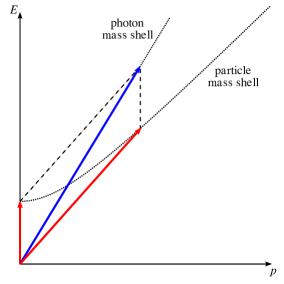
(a)

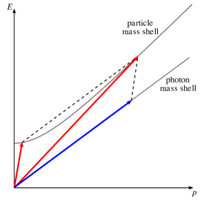
(b)

Figure 1: Mass shells and momentum vectors for one-to-two processes when the limiting particle speed $c_{p}$ differs from the speed of light $c_{\gamma}=E_{\gamma}/p_{\gamma}$. (a) When $c_{\gamma}>c_{p}$ (or, equivalently, $\beta>0$), a photon (blue) can decay into two massive charged particles (red). (b) When $c_{\gamma}<c_{p}$ ($\beta<0$), a charged particle with sufficiently high energy (red) can decay to a charged particle of lower energy (red) and a photon (blue).

It is important to note that each of these processes is sensitive to $\beta$ values of only one sign. The directions $k_{a}$ of bumblebee photon propagation are those for which $\tilde{\eta}^{ab}k_{a}k_{b}=0$. Denoting $k_{\mu}=(\omega/c_{p},\vec{k})$, where $c_{p}$ is the limiting speed of the particle species, we see that this “null condition” is equivalent to

$$\omega^{2}=c_{p}^{2}(\vec{k}^{2}+\beta(\bar{B}^{a}k_{a})^{2})$$ (39)

This implies that if $\beta>0$, we will have $c_{\gamma}=\omega/|\vec{k}|>c_{p}$, and photons of sufficiently high energy can decay to charged particles and anti-particles. Similarly, if $\beta<0$, we will have $c_{\gamma}<c_{p}$, and charged particles of sufficiently high energy will lose energy to vacuum Čerenkov radiation.

What are the threshold energies for these processes? Denoting $\vec{k}=k\hat{k}$, where $\hat{k}$ is a unit vector, we find that the photon dispersion relation (39) above can written as

$$\omega=c_{p}k\left[\frac{\beta\bar{B}^{0}(\vec{B}\cdot\hat{k})+\sqrt{1+\beta(-(\bar{B}^{0})^{2}+(\vec{B}\cdot\hat{k})^{2})}}{1-\beta(\bar{B}^{0})^{2}}\right]$$ (40)

In the case of photon decay, the threshold photon energy $E_{d0}$ will be that for which a photon with four-momentum $\hbar c_{p}k_{a}$ can decay into a particle-antiparticle pair, with each particle having four-momentum $p_{a}=\frac{1}{2}\hbar c_{p}k_{a}$ and rest mass $m$. Taking the norm of $p_{a}$ with respect to $\tilde{\eta}^{ab}$, we find that the four-momentum of the each particle must satisfy

$$p_{a}p_{b}\tilde{\eta}^{ab}=p^{a}p_{a}+\beta(\bar{B}^{a}p_{a})^{2}=-m^{2}c_{p}^{4}+\beta(\bar{B}^{a}p_{a})^{2}.$$ (41)

The left-hand side of this equation vanishes (since $p_{a}p_{b}\tilde{\eta}^{ab}\propto k_{a}k_{b}\tilde{\eta}^{ab}$). Rewriting the right-hand side in terms of $k_{\mu}$, and defining $n^{a}\equiv\sqrt{|\beta|}\bar{B}^{a}$, we find that at threshold

$$(n^{0}\omega+(\vec{n}\cdot\hat{k})c_{p}k)^{2}=\left(\frac{2mc_{p}^{2}}{\hbar}\right)^{2}.$$ (42)

Applying the dispersion relation (40) then yields a threshold energy of

$$E_{d0}(\hat{k})=2mc_{p}^{2}\left|\frac{n^{0}-(\vec{n}\cdot\hat{k})\sqrt{1-(n^{0})^{2}+(\vec{n}\cdot\hat{k})^{2}}}{(n^{0})^{2}-(\vec{n}\cdot\hat{k})^{2}}\right|.$$ (43)

In the limit of the components of $n^{\mu}$ being much less than unity, this simplifies to

$$E_{d0}(\hat{k})\approx\frac{2mc_{p}^{2}}{|n^{0}+\vec{n}\cdot\hat{k}|}.$$ (44)

In the case of vacuum Čerenkov radiation, the threshold energy is best found using a geometric argument (see Figure 1.) Since momentum is conserved, the four-momentum of the photon will “connect” two points on the charged-particle mass shell. The threshold energy $E_{c0}$ for vacuum Čerenkov radiation is therefore that point on the mass shell at which the slope of the tangent line ($\mathrm{d}E_{p}/\mathrm{d}p_{p}$) equals the slope of the photon mass shell: at any energy on the charged-particle mass shell with $E_{i}>E_{c0}$, we can draw a secant line with the same slope as the photon mass shell that will intersect the charged-particle mass shell at a lower energy $E_{f}<E_{i}$. This will not, however, be possible for $E_{i}<E_{c0}$. Performing this calculation, we find that the threshold energy $E_{c0}$ for a particle of mass $m$ is given by

$$E_{c0}(\hat{k})=\frac{mc_{p}^{2}}{\sqrt{1-c_{\gamma}^{2}(\hat{k})/c_{p}^{2}}}$$ (45)

where the (direction-dependent) speed of light $c_{\gamma}(\hat{k})$ is given dividing $\omega$ by $k$ in (40). Plugging this in, we find that the threshold energy is given by

$$E_{c0}(\hat{k})=mc_{p}^{2}\left|\frac{(\vec{n}\cdot\hat{k})-n^{0}\sqrt{1-(n^{0})^{2}+(\vec{n}\cdot\hat{k})^{2}}}{(n^{0})^{2}-(\vec{n}\cdot\hat{k})^{2}}\right|.$$ (46)

where we have again used the rescaled vector $n^{a}=\sqrt{|\beta|}\bar{B}^{a}$. If we again take the limit of small $n^{\mu}$, this reduces to

$$E_{c0}(\hat{k})\approx\frac{mc_{p}^{2}}{|n^{0}+\vec{n}\cdot\hat{k}|}.$$ (47)

In the case $\beta<0$, the detection of a charged particle with energy $E_{p}$ and mass $m$ propagating in the direction $\hat{k}$ implies that the Čerenkov threshold energy $E_{c0}(\hat{k})$ for that direction is greater than $E_{p}$. Thus, we can say that such a detection restricts the components of $n^{a}$ to lie in the region

$$|n^{0}+\vec{n}\cdot\hat{k}|<\frac{mc_{p}^{2}}{E_{p}}.$$ (48)

This region is a thickened plane in $n^{\mu}$-space, with a total thickness of $2mc_{p}^{2}/E_{p}$. Multiple detections of charged particles coming from different directions $\hat{k}$ can then constrain the parameters of our theory to a finite region of $n^{\mu}$-space. Note that the quantity appearing on the right-hand side of (48) is simply the inverse of boost factor $\gamma$ of the charged particle detected.

Similarly, when $\beta>0$, the detection of a photon with energy $E_{\gamma}$ propagating in the direction $\hat{k}$ implies that the components of $n^{a}=\sqrt{|\beta|}\bar{B}^{a}$ satisfy

$$|n^{0}+\vec{n}\cdot\hat{k}|<\frac{2m_{e}c_{p}^{2}}{E_{\gamma}}.$$ (49)

Here, $m_{e}$ is the electron mass: the $\gamma\to e^{-}e^{+}$ process will have a lower threshold than any other photon decay channel. Once again, high-energy photons from various directions can then constrain us to a finite region of $n^{\mu}$-space.

The rate of energy loss for vacuum Čerenkov processes has been calculated by Altschul Altschul (2008). In particular, a charged particle with energy just above threshold ($E_{p}=E_{c0}+\Delta E$, with $\Delta E\ll E_{c0}$) will emit a photon with $E_{\gamma}>\Delta E$ with a decay rate of

$$\Gamma=\alpha Z^{2}m^{2}\frac{(\Delta E)^{2}}{2E_{p}^{3}},$$ (50)

where $\alpha$ is the fine structure constant, $Z$ is the particle’s charge, and $m$ is its rest mass. The mean free path of such a particle (assuming it to be moving with velocity $v\approx c_{p}$) can then be estimated as $\ell=c_{p}/\Gamma$. At higher energies, the charged particle will mainly lose energy to larger numbers of lower-energy photons, rather than a single photon that brings it below threshold. This process causes the energy to decrease even more rapidly; we should therefore view the estimate $\ell$ above as an upper bound on the mean free path for a particle with energy $E_{p}$.

In the case of photon decay, an exact expression for the lifetime of the photon is not yet known. However, we can estimate (see the Appendix) that the decay rate for photons above threshold energy $E_{d0}$ will be on the order of magnitude of

$$\Gamma\sim\alpha\beta\mathcal{B}^{2}E_{\gamma}\sqrt{1-\frac{E_{d0}^{2}}{E_{\gamma}^{2}}},$$ (51)

where $\alpha$ is the fine structure constant and $\mathcal{B}$ is a quantity of the same order of magnitude as the components of $\bar{B}^{a}$. Using this estimate, one can then calculate a mean free path for photons as in the case of vacuum Čerenkov radiation. Roughly speaking, a photon well above threshold will have a mean free path of order $(\alpha\beta\mathcal{B}^{2})^{-1}$ times its Compton wavelength; if the photon is only barely above threshold, with energy $E_{\gamma}=(1+\epsilon)E_{d0}$, its mean free path (in Compton wavelengths) is reduced by a factor of approximately $\sqrt{\epsilon}$.

IV Experimental constraints

In general, the most stringent limits on the components of $(k_{F})^{abcd}$ are those that arise from searches for vacuum birefringence Kostelecký and Russell . However, the vanishing of the matrices $(\tilde{\kappa}_{e+})^{ij}$ and $(\tilde{\kappa}_{o-})^{ij}$ (37a) implies that in our case, bumblebee photons do not experience vacuum birefringence. We must thus turn to other experimental means of searching for Lorentz violation in the photon sector. In the following subsections, we will discuss limits arising from rotating electromagnetic resonator experiments, particle accelerator experiments, and cosmic-ray observations.

IV.1 Resonator experiments

If the Maxwell field is Lorentz-invariant, the frequencies of its modes in a resonant cavity will be independent of the cavity’s orientation in space. However, if the photon field propagates at different speeds in different directions, it is not hard to see that the resonant frequencies of the cavity can change if the cavity’s orientation changes: this frequency depends on the “speed of light” in the cavity, and this speed is direction-dependent in our model if $\beta\neq 0$ and $\vec{B}\neq 0$. The magnitude of this frequency shift for a given set of matrices $\tilde{\kappa}_{e\pm}$ and $\tilde{\kappa}_{o\pm}$ was calculated for a general cavity mode and geometry in Kostelecký and Mewes (2002). In practise, this frequency shift is usually measured by setting up two identical cavities, oriented at right angles to each other, and rotating these two cavities together. A difference in the speed of light within the plane of rotation would then show up as a “beat” between the frequencies of the two cavities, modulating at twice the frequency of rotation. By looking for these “beats” at various points in the Earth’s rotation and revolution, all eight independent components of the SME matrices $(\tilde{\kappa}_{e-})^{ij}$ and $(\tilde{\kappa}_{o+})^{ij}$ can in principle be measured.

Sensitive measurements of the components of $(\tilde{\kappa}_{e-})^{ij}$ and $(\tilde{\kappa}_{o+})^{ij}$ have been performed by Herrmann et al. Herrmann et al. (2008) and by Eisele, Nevsky and Schiller Eisele et al. (2009). Both groups have bounded the components of $(\tilde{\kappa}_{e-})^{ij}$ to be $\mathcal{O}(10^{-17})$ or less, and those of $(\tilde{\kappa}_{o+})^{ij}$ to be $\mathcal{O}(10^{-13})$ or less. We can translate these measured bounds into a rough estimate of the bounds on our parameters $\beta$ and $\bar{B}^{\mu}$; given the dependencies given in (37b) and (37c), we would expect the magnitude of $n^{0}=\sqrt{|\beta|}\bar{B}^{0}$ to be bounded below approximately $3\times 10^{-5}$, and the components of $\vec{n}$ to be approximately $3\times 10^{-9}$ or less.

It is important to note, however, that both of the above mentioned groups Herrmann et al. (2008); Eisele et al. (2009) derived their respective bounds from their experimental data under the assumption that all eight independent components of $(\tilde{\kappa}_{e-})^{ij}$ and $(\tilde{\kappa}_{o+})^{ij}$ could be varied independently. In our model, this is not the case; rather, as noted above, we have a four-dimensional parameter space (along with an additional discrete parameter). A more thorough analysis should thus involve a (non-linear) regression on this parameter space, starting from the experimental data.

	Best Fit				$1\sigma$ Conf. Intervals
	$\beta>0$		$\beta<0$		$\beta>0$	$\beta<0$
$n^{0}$	$0$.	$69$	$-1$.	$61$	$[-2.16,3.54]$	$[-4.43,1.21]$
$n^{X}$	$4$.	$00$	$-2$.	$06$	$[0.50,6.26]$	$[-4.21,0.52]$
$n^{Y}$	$1$.	$30$	$3$.	$61$	$[-1.57,3.83]$	$[0.07,5.76]$
$n^{Z}$	$-2$.	$39$	$-1$.	$46$	$[-5.29,0.52]$	$[-3.88,0.96]$

Table 1: Best fits and approximate $1\sigma$ confidence intervals for $n^{0}$ (times $10^{-4}$) and $\vec{n}$ (times $10^{-8}$) in the standard Sun-centred frame, derived from the data of Stanwix et al. Stanwix et al. (2006).

To perform such an analysis, we turn to the data of Stanwix et al. In Table I of Stanwix et al. (2006), the time-variation of the above-mentioned “beat” amplitudes are given. Applying a non-linear regression to these amplitudes gives the results shown in Table 1 for the components $n^{\mu}$ in the Sun-centred frame. The best fit is found to occur for $\beta>0$; however, a region of parameter space with $\beta<0$ also falls in the overall $1\sigma$ confidence region. The approximate dimensions of the one-sigma confidence contour in both the $\beta>0$ and $\beta<0$ regions of parameter space are also given in Table 1. The point $n^{\mu}=(0,0,0,0)$ lies approximately on the 75% confidence contour. While this might seem suggestive of a non-zero Lorentz-violating effect, such a confidence level can hardly be thought of as conclusive, especially considering that Stanwix et al. viewed as spurious the $2\sigma$ and $3\sigma$ signals found via their original analysis (with SME coefficients assumed to be independent.) We must therefore conclude that resonator experiments have not yet observed a signal compatible with the generalized bumblebee model.

IV.2 Accelerator physics

As noted above, vacuum Čerenkov radiation and photon decay, though kinematically forbidden in conventional theories, are both allowed above a certain energy threshold in the presence of Lorentz invariance in the photon sector. In the bumblebee photon case, this threshold will decrease as the components of the rescaled vector $n^{a}=\sqrt{|\beta|}\bar{B}^{a}$ increase. Direct observations of high-energy particles can therefore help us constrain our theory.

An analysis along these lines has been performed by Hohensee et al. Hohensee et al. (2009), through analysis of the operation of the LEP experiment and the Tevatron. In the case of vacuum Čerenkov radiation, they note that a threshold energy $E_{c0}$ more than a few MeV below the electron and positron beam energies at LEP ($E_{\text{LEP}}=104.5$ GeV) would have caused beam energy losses significant enough to be immediately apparent. In our case, this implies that

$$|n^{0}+\vec{n}\cdot\hat{k}|<\frac{m_{e}}{E_{\text{LEP}}}\approx 4.9\times 10^{-6}.$$ (52)

Moreover, from the known bounds due to resonator experiments (above), we know that the components of $\vec{n}$ are of order $10^{-8}$. This therefore implies that in the case $\beta<0$, we must have $|n^{0}|<4.9\times 10^{-6}$.

For the case of photon decay, Hohensee et al. note that a significant fraction of predicted high-energy photons ($E_{\gamma}\gtrsim 300$ GeV) have been observed in the D0 detector at Fermilab (specifically, in the study of isolated-photon production with an associated jet.) This implies that the threshold energy for photon decay cannot greatly exceed 300 GeV; again using the bounds on the components of $\vec{n}$ from resonator experiments, we find that in the case $\beta>0$ we must have

$$|n^{0}|\lesssim\frac{2m_{e}}{E_{\gamma}}\approx 3.4\times 10^{-6}.$$ (53)

More recently, work by Altschul Altschul has extended these bounds by examining the amount of synchrotron radiation observed at LEP. The argument proceeds similarly to the analysis of vacuum Čerenkov radiation in LEP, given above. In a Lorentz-violating theory, the velocity of a relativistic charged particle moving in a uniform magnetic field will deviate from the “expected” velocity (i.e., that in the absence of Lorentz violation) by $\delta v=\tilde{\kappa}$, where $\tilde{\kappa}$ is a linear combination (with coefficients of order unity) of the Lorentz-violating coefficients $(\tilde{\kappa}_{e-})^{ij}$, $(\tilde{\kappa}_{o+})$, and $\tilde{\kappa}_{\text{tr}}$ Altschul (2005). The fractional deviation of the synchrotron power radiated from its expected value is then given by of order

$$\frac{\Delta P}{P}=8\gamma^{2}\tilde{\kappa},$$ (54)

where $\gamma$ is the boost factor of the relativistic particle. When we integrate this power deviation over a full cycle of the charged particle, the parity-odd coefficients must drop out due to symmetry; thus, only $(\tilde{\kappa}_{e\pm})^{ij}$ and $\tilde{\kappa}_{\text{tr}}$ can in principle contribute to the integrated synchrotron power loss.

The greatest boost factor $\gamma$ of particles achieved at LEP was above $2\times 10^{5}$; the integrated power loss of particles in the storage rings at LEP was measured to agree with the predictions of standard (non-Lorentz-violating) electrodynamics to within a fractional precision of $|\Delta P|/P<2\times 10^{-4}$ Altschul . We can thus conclude that

$$|\tilde{\kappa}|<\frac{1}{8\gamma^{2}}\frac{|\Delta P|}{P}\approx 6\times 10^{-16}$$ (55)

Since resonator experiments bound the components of $(\tilde{\kappa}_{e-})^{ij}$ to an order of magnitude below this, this bound is therefore only a bound on $\tilde{\kappa}_{\text{tr}}$. In our case, $\tilde{\kappa}_{\text{tr}}$ is given by equation (37d). We can thus conclude that the known bounds on synchrotron radiation at LEP limit only the value of $\tilde{\kappa}_{\text{tr}}$; specifically,

$$|n^{0}|<\sqrt{2|\tilde{\kappa}_{\text{tr}}|}<3.5\times 10^{-8}.$$ (56)

Note that this is a two-sided bound: since LEP is sensitive to $\Delta P/P$ being either positive or negative, and since the sign of $\Delta P/P$ is dependent on $\tilde{\kappa}_{\text{tr}}$, then LEP measurements bound $\tilde{\kappa}_{\text{tr}}$ both above and below zero. In the current model, this means that $n^{0}$ is bounded both for $\beta>0$ and $\beta<0$.

This bound is comparable to the current bounds on the spatial components of $\vec{n}$ obtainable from resonator experiments. However, this bound should be taken correct only to within an order of magnitude, due to our lack of knowledge about the precise functional form of $\tilde{\kappa}$ in our theory. A more precise estimate would involve a full calculation of the rate of synchrotron radiation in our model; however, such a calculation is outside the scope of this paper.

IV.3 Cosmic ray observations

While man-made particle accelerators can impart very high energies to particles, it is well-known that “natural particle accelerators” elsewhere in the Universe put these efforts to shame; cosmic rays have been observed with energies of up to eight orders of magnitude more energy than the most energetic particles created in the laboratory to date. Since our bounds on the parameters of our theory scale inversely with the energies of observed particles, we will find that subject to some caveats (detailed below) cosmic ray observations give us the best bounds on the components of $n^{\mu}$.

In the case of vacuum Čerenkov radiation, the Pierre Auger Collaboration has observed a few dozen cosmic ray showers with total energies above 57 EeV Abraham et al. (2008). It is generally assumed that the primary particles for such cosmic ray showers are hyperrelativistic protons or nuclei. In our case, the inequality (48) becomes more restrictive as the mass of the primary particle decreases. Thus, if we wish to place conservative bounds on the parameters of the theory, we should assume that the primary is a fairly heavy nucleus. It is unlikely, however, that these primaries are significantly heavier than ${}^{56}\text{Fe}$. We therefore assume that all the events listed in Abraham et al. (2008) have a primary mass of $M_{p}c_{p}^{2}=52.1$ GeV. If these events were to later be discovered to have a smaller mass $M^{\prime}_{p}$, it would simply rescale our limits on $n^{\mu}$ by a factor of $M^{\prime}_{p}/M_{p}$.

	Cosmic rays		VHE photons
$|n^{0}|$	$6$.	$8\times 10^{-10}$	$2$.	$1\times 10^{-8}$
$|n^{X}|$	$5$.	$6\times 10^{-10}$	$6$.	$7\times 10^{-8}$
$|n^{Y}|$	$8$.	$2\times 10^{-10}$	$3$.	$3\times 10^{-8}$
$|n^{Z}|$	$14$.	$6\times 10^{-10}$	$5$.	$3\times 10^{-8}$
	$19$.	$9\times 10^{-19}$	$46$.	$6\times 10^{-16}$
$n^{\mu}n_{\mu}$	$-2$.	$3\times 10^{-19}$	$-3$.	$3\times 10^{-16}$
$V_{n}$	$6$.	$0\times 10^{-37}$	$2$.	$7\times 10^{-30}$

Table 2: Bounds placed on the components of $n^{\mu}\equiv\sqrt{|\beta|}\bar{B}^{a}$ in the Sun-centred frame by cosmic-ray observations ($\beta<0$) and high-energy gamma-ray observations ($\beta>0$).

The 27 events listed in Abraham et al. (2008) thus disallow large volumes of parameter space. The remaining, allowed region of parameter space is a complicated non-uniform polychoron, symmetric with respect to reflection about the origin. The maximum allowed magnitudes of each of the components of $n^{\mu}$ are listed in Table 2, along with the maximum and minimum allowed values of the norm of $n^{a}$, and the volume $V_{n}$ of the allowed polychoron.

In the case $\beta>0$, we would expect to see a (possibly direction-dependent) cutoff in the very high-energy (VHE) gamma-ray spectrum. Over the past decade, gamma-ray observatories such as HESS, VERITAS and MAGIC have catalogued several dozen VHE gamma-ray sources, and in many cases have been able to associate these sources with known objects (either in the Milky Way or extragalactic.) However, two problems arise when attempting to use these sources to bound the parameters of our theory. The first is simply a matter of orders of magnitude; the ratio of the energy of these gamma-rays to the electron mass is two orders of magnitude smaller than the boost factor of the charged particles that make up cosmic rays. The highest-energy photons detected thus far have energies of order 75 TeV, yielding a bounding factor $2m_{e}c_{p}^{2}/E_{\gamma}$ of approximately $10^{-8}$; by contrast, the inverses of the boost factors for the charged-particle gamma rays observed by the Pierre Auger Observatory are of order $10^{-10}$. Thus, we cannot expect nearly so tight a bound on the components of $n^{\mu}$ as we obtained in the case $\beta<0$.

Second, the vast majority of the sources we can reliably use for this purpose lie in the plane of the Milky Way. Most known extragalactic sources of VHE gamma rays are associated with blazars located outside of the Local Supercluster, with non-negligible cosmological redshift ($z\gtrsim 0.05$.) Once cosmological effects become non-negligible, our assumptions of nearly-flat metric (8) and nearly-constant vector field (9) can no longer be expected to hold. Instead, we would expect that $g^{ab}$ would be approximate a Friedman-Robertson-Walker solution, and that the value of $B^{a}$ would be subject to cosmological evolution. This would cause significant deviations from the predictions of Section III.3, which were predicated on $\tilde{\eta}^{ab}$ being constant throughout the propagation of the photon. For the purposes of this paper, we will therefore limit ourselves to VHE gamma-ray sources known or suspected to be within the Local Supercluster.

Name	$RA$ (${}^{\text{o}}$)		$\delta$ (${}^{\text{o}}$)		$E_{\text{max}}$ (TeV)		Ref.
Crab Nebula	83.	6	22.	01	75		Aharonian et al. (2004)
RX J1713.7-3946	258.	4	$-39$.	76	47		Aharonian et al. (2007a)
Vela X	128.	8	$-45$.	60	45		Aharonian et al. (2006a)
HESS J1825-137	276.	5	$-13$.	76	40		Aharonian et al. (2006b)
MSH 15-52	228.	5	$-59$.	16	40		Aharonian et al. (2005a)
Galactic Centre	266.	3	$-29$.	00	32		Aharonian et al. (2009a)
HESS J1809-193	272.	6	$-19$.	30	30		Aharonian et al. (2007b)
HESS J1708-443	257.	0	$-44$.	35	20		Hoppe et al. (2009)
LS 5039	276.	6	$-14$.	85	20		Aharonian et al. (2006c)
RCW 86	220.	7	$-62$.	45	20		Aharonian et al. (2009b)
HESS J1616-508	244.	1	$-50$.	90	20		Aharonian et al. (2006b)
HESS J1813-178	273.	4	$-17$.	84	20		Aharonian et al. (2006b)
M87	187.	7	12.	39	20		Aharonian et al. (2006d)
Westerlund 2	155.	8	$-57$.	76	18		Aharonian et al. (2007c)
HESS J1837-069	279.	4	$-6$.	95	15		Aharonian et al. (2006b)
Kookaburra	214.	5	$-60$.	98	15		Aharonian et al. (2006e)
HESS J1718-385	259.	5	$-38$.	55	15		Aharonian et al. (2007b)
RX J0852.0-4622	133.	0	$-46$.	37	10		Aharonian et al. (2005b)
Cassiopeia A	350.	9	58.	82	10		Albert et al. (2007)
HESS J1702-420	255.	7	$-42$.	02	10		Aharonian et al. (2006b)
HESS J1804-216	271.	1	$-21$.	70	10		Aharonian et al. (2006b)
CTB 37A	258.	6	$-38$.	57	10		Aharonian et al. (2008)
Centaurus A	201.	4	43.	02	5		Aharonian et al. (2009c)
AE Aquarii	310.	0	$-0$.	87	3	.5	Meintjes et al. (1992)

Table 3: VHE gamma-ray sources with significant observed luminosity over 10 TeV. Shown are the names of the sources, their right ascension and declination (in degrees), and $E_{\text{max}}$, the approximate maximum energy of gamma rays observed in their spectra. The sources AE Aquarii and Centaurus A have $E_{\text{max}}<10$ TeV but are included due to their higher galactic latitude ($-24.42^{\text{o}}$ and $19.42^{\text{o}}$, respectively); see text.

With these caveats in mind, we proceed. A survey of the literature reveals 22 known VHE gamma-ray sources with significant flux at energies greater than 10 TeV (see Table 3.) Only one of these sources, M87 Aharonian et al. (2006d), is extragalactic (with $b=74.49^{\text{o}}$). To improve our bounds in the directions orthogonal to the galactic plane, we therefore include two lower-energy sources: the radio galaxy Centaurus A Aharonian et al. (2009c), with galactic latitude $b=-24.42^{\text{o}}$, and the cataclysmic variable AE Aquarii Meintjes et al. (1992), with $b=19.42^{\text{o}}$. The resulting bounds are shown in Table 2. As expected, they are significantly less stringent than the bounds imposed by charged-particle cosmic ray observations; however, they are still competitive with the limits imposed on the components of $\vec{n}$ by laboratory and accelerator experiments, and are more stringent in the case of $n^{0}$.

V Discussion

Laboratory experiments (both electromagnetic resonators and bounds from accelerator physics) limit the components of $n^{\mu}$ to the $10^{-8}$ level. In the case $\beta<0$, cosmic-ray observations push these bounds down $\mathcal{O}(10^{-10})$ for all components of $n^{\mu}$; for $\beta>0$, similar observations bound all the components of $n^{\mu}$ to the $10^{-8}$ level.

A few notes concerning the above bounds are in order. First, the bounds extracted from the regression in Section IV.1 are not based on the current strongest bounds on Lorentz violation in the photon sector, but rather on older work with more detailed reporting of data. One would expect that if the data underlying the most sensitive experiments to date Herrmann et al. (2008); Eisele et al. (2009) were analyzed in this way, our sensitivity to the components of $n^{\mu}$ would increase by approximately a factor of three (i.e., half an order of magnitude.)

The great majority of the cosmic-ray sources and events used in Section IV.3 are in the Southern Celestial Hemisphere. This is simply due to the locations of the observatories in question. In the case of high-energy charged particles, the Pierre Auger Observatory (located in Argentina) does not yet have a Northern-Hemisphere counterpart; Pierre Auger North, a planned counterpart in Colorado, will not see “first light” for some years. In the case of high-energy gamma rays, this asymmetry is simply due to the fact that the HESS telescope (located in Namibia) has been in operation longer than the similar MAGIC and VERITAS telescopes (located in the Canary Islands and Arizona, respectively.) As these latter two telescopes and the air-shower arrays MILAGRO (New Mexico), AS$\gamma$ (Tibet), and ARGO (Tibet) report more high-energy sources (especially in the region of the galactic plane lying in the Northern Celestial Hemisphere), we can expect these bounds to become more symmetric.

Finally, it is important to note that there are fundamental limits on how well gamma-ray experiments can bound the parameters of our theory. Photons with sufficiently high energies can interact with background radiation (particularly the cosmic microwave background) and produce electron-positron pairs Gould and Schréder (1966). In particular, the “gamma-ray horizon” for $\sim 100$ TeV gamma rays is approximately the size of the Local Supercluster, and for $\sim 1$ PeV gamma rays is approximately the size of the Milky Way. This pair-production attenuation therefore places fundamental bounds on the region of parameter space that can be bounded by gamma-ray observations: we do not expect to get extremely high-energy gamma rays from outside our own galaxy, but our bounds on the component of $\vec{n}$ orthogonal to the galactic plane will generically be insensitive to sources from within the Galaxy.

Appendix A Photon Lifetime

In using particle physics to place bounds on Lorentz-violating theories, it is informative to examine the mean free paths of particles or, equivalently, their lifetimes. The rate of energy loss to vacuum Čerenkov radiation in a general Lorentz-violating theory has been previously derived Altschul (2008). However, the decay $\gamma\to e^{+}e^{-}$, as occurs in our case when $\beta>0$, is less well-understood. The full quantum theory of Lorentz-violating photons is not yet known, and so a calculation of the exact photon decay rate is impossible. However, it is well-known that when certain Lorentz-violating coefficients are sufficiently small, they can be “moved” between sectors via redefinitions of the metric (or, equivalently, redefinitions of the coordinates.) In particular, for a theory of Lorentz-violating photons without vacuum birefringence on a flat metric, it is possible to shift the Lorentz-violating coefficients entirely into the electron sector instead Kostelecký and Lehnert (2001). The quantum field theory of Lorentz-violating electrons being much better understood Colladay and Kostelecký (2001), we pursue this tactic. We will see that such a technique will only yield decay rates that are accurate to first order in $\beta$; however, this calculation will still be valuable in estimating the mean free paths of Lorentz-violating photons.

A similar calculation for “isotropic Lorentz-violating photons” has been performed by Hohensee et al. Hohensee et al. (2009); we will follow their techniques here. For consistency with this paper and Colladay and Kostelecký (2001), we use a metric with signature $(+,-,-,-)$. In particular, when switching to this sign convention, our definition of $\tilde{\eta}^{ab}$ will change; in this sign convention, a metric of the form

$$\tilde{\eta}^{ab}=\eta^{ab}-\beta\bar{B}^{a}\bar{B}^{b}$$ (57)

is physically equivalent to the metric used in the previous sections.

We start with the “Lorentz-violating QED” Lagrangian for bumblebee photons minimally coupled to an electron field $\psi$ in flat spacetime:

$$\mathcal{L}=\frac{i}{2}\bar{\psi}\gamma^{a}\overset{\leftrightarrow}{D}_{a}\psi-m\bar{\psi}\psi-\frac{1}{4}\tilde{\eta}^{ab}\tilde{\eta}^{cd}F_{ac}F_{bd},$$ (58)

with $\tilde{\eta}^{ab}$ defined as in (57). The process used by Hohensee et al. to derive the photon lifetime consists of several steps:

1. We redefine the metric so that the “photon metric” $\tilde{\eta}^{ab}$ is the “true metric” of the theory. Since the gamma matrices in the electron kinetic term are defined with respect to the original metric $\eta^{ab}$ (i.e., $\{\gamma^{a},\gamma^{b}\}=2\eta^{ab}$), we must rewrite these matrices in terms of new gamma matrices $\tilde{\gamma}^{a}$ defined such that $\{\tilde{\gamma}^{a},\tilde{\gamma}^{b}\}=2\tilde{\eta}^{ab}$. To first order in $\beta$, these matrices are related by

   $$\gamma^{a}=\tilde{\gamma}^{a}+\frac{\beta}{2}\bar{B}^{a}\bar{B}^{b}\tilde{\eta}_{bc}\tilde{\gamma}^{c}.$$ (59)

   Applying this definition to our Lagrangian, we find that our new Lagrangian is

   $$\mathcal{L}=\frac{i}{2}\bar{\psi}\left(\tilde{\gamma}^{a}+\frac{\beta}{2}\bar{B}^{a}\bar{B}^{b}\tilde{\gamma}_{b}\right)\overset{\leftrightarrow}{D}_{a}\psi-m\bar{\psi}\psi-\frac{1}{4}F_{ab}F^{ab}$$ (60)

   where indices are now raised and lowered with the metric $\tilde{\eta}^{ab}$. We will hereafter “drop the tildes” for notational convenience.

2. The kinetic term for the electron now contains non-standard time derivatives; these must be eliminated to successfully quantize the theory Kostelecký and Lehnert (2001). To do this, we define a new spinor field $\chi$ such that $\psi=A\chi$, where the matrix $A$ satisfies

   $$A^{\dagger}\gamma^{0}\left(\gamma^{0}+\frac{\beta}{2}\bar{B}^{0}\bar{B}^{b}\gamma_{b}\right)A=\mathbf{1}.$$ (61)

   To first order in $\beta$, this implies that

   $$A=\mathbf{1}-\frac{\beta}{4}\bar{B}^{0}\bar{B}_{a}\gamma^{0}\gamma^{a}.$$ (62)

   Rewriting the Lagrangian in terms of $\chi$ then yields

   $$\mathcal{L}=\frac{i}{2}\hat{\eta}^{ab}\bar{\chi}\gamma_{a}\overset{\leftrightarrow}{D}_{b}\chi-\hat{m}\bar{\chi}\chi-\frac{1}{4}F_{ab}F^{ab},$$ (63)

   where

   $$\hat{\eta}^{ab}=\eta^{ab}-\frac{\beta}{2}\left((\bar{B}^{0})^{2}\eta^{ab}+2\bar{B}^{0}\bar{B}^{[a}\eta^{b]0}-\bar{B}^{a}\bar{B}^{b}\right)$$ (64)

   and

   $$\hat{m}=m\left(1-\frac{\beta}{2}(\bar{B}^{0})^{2}\right).$$ (65)

3. Write down the invariant matrix element $\mathcal{M}$. Using the photon and electron polarizations defined in Hohensee et al. (2009), we find this to be given by

   $$i\mathcal{M}_{rs}=-ie\epsilon_{a}(p)\hat{\eta}^{ab}\bar{u}^{(r)}(q)\gamma_{b}v^{(s)}(k)$$ (66)

   where $p^{a}$ is the incoming photon momentum, $\epsilon_{a}(p)$ is its polarization, $q^{a}$ and $k^{a}$ are the outgoing electron and positron momenta respectively, and $\bar{u}^{(r)}(q)$ and $v^{(s)}(k)$ are their respective polarization states. To obtain the photon lifetime, we will need to sum over the final fermion polarization states and average over photon polarization states; using the trace identities derived in Colladay and Kostelecký (2001), this yields

   $$\overline{|\mathcal{M}|^{2}} =\frac{1}{2}\sum_{\epsilon}\sum_{r,s}|\mathcal{M}_{r,s}|^{2}$$

   $$=2e^{2}\big{(}\hat{\eta}^{ab}\hat{\eta}_{ab}(\hat{m}^{2}+\hat{\eta}^{e}{}_{c}\hat{\eta}_{ed}q^{c}k^{d})$$

   $$\mspace{150.0mu}{}-2\hat{\eta}_{a}{}^{b}\hat{\eta}_{cb}\hat{\eta}^{ad}\hat{\eta}^{ce}q_{d}k_{e}\big{)}.$$ (67)

   We have used the spinor normalization conventions chosen in Hohensee et al. (2009) (i.e., $N(\vec{q})=2E_{q}$ and similarly for $k$.)

4. Integrate over the final electron and positron momenta to obtain the photon lifetime as a function of its energy $E_{\gamma}$ and propagation direction $\hat{p}$:

   $$\Gamma(\hat{p})=\frac{1}{4\pi^{2}}\frac{1}{2E_{\gamma}}\int\frac{\mathrm{d}^{3}\vec{q}}{2E_{q}}\frac{\mathrm{d}^{3}\vec{k}}{2E_{k}}\overline{|\mathcal{M}|^{2}}\delta^{4}(p^{\mu}-q^{\mu}-k^{\mu})$$ (68)

I have as yet been unable to derive a closed-form analytical expression for this lifetime. However, an order-of-magnitude estimate of the photon decay rate may be obtained by estimating the quantity $\overline{|\mathcal{M}|^{2}}/4E_{q}E_{k}$ for an on-shell decay and multiplying this quantity by the allowed volume of phase space; in other words,

$$\int\frac{\mathrm{d}^{3}\vec{q}}{2E_{q}}\frac{\mathrm{d}^{3}\vec{k}}{2E_{k}}\overline{|\mathcal{M}|^{2}}\delta^{4}(p^{\mu}-q^{\mu}-k^{\mu})\\ =\left\langle\frac{\overline{|\mathcal{M}|^{2}}}{4E_{q}E_{k}}\right\rangle\times\int\mathrm{d}^{3}\vec{q}\,\mathrm{d}^{3}\vec{k}\,\delta^{4}(p^{\mu}-q^{\mu}-k^{\mu})$$ (69)

This equation can be thought of as defining the quantity in angle brackets above. To estimate its order of magnitude, we can use the dispersion relation for the electrons in this theory,

$$\hat{\eta}_{ac}\hat{\eta}_{b}{}^{c}k^{a}k^{b}=\hat{m}^{2},$$ (70)

along with momentum conservation, $p^{a}=k^{a}+q^{a}$, to put (67) in the form

$$\overline{|\mathcal{M}|^{2}}=2e^{2}\Big{[}2\beta E_{\gamma}^{2}\left(-2\bar{B}^{0}\vec{B}\cdot\hat{p}+(\vec{B}\cdot\hat{p})^{2}\right)\\ +2(1-\beta(\bar{B}^{0})^{2})\hat{m}^{2}+\beta(\bar{B}_{a}k^{a})^{2}+\beta(\bar{B}_{a}q^{a})^{2}\Big{]}\\ +\mathcal{O}(\beta^{2})$$ (71)

All of these terms except for the last two are constant over the mass shell. To estimate the order of magnitude of these last two terms, we note that the electron dispersion relation satisfies $E_{k}^{2}-\vec{k}^{2}=m^{2}+\mathcal{O}(\beta)$; thus,

$$\beta(\bar{B}_{a}k^{a})^{2} =\beta(\bar{B}^{0}E_{k}-|\vec{B}||\vec{k}|\cos\theta)^{2}$$

$$\sim\beta\left(\bar{B}^{0}E_{k}-|\vec{B}|\sqrt{E_{k}^{2}-m^{2}}\right)^{2}$$ (72)

where we have discarded the $\cos\theta$ term because it is of order unity. We can further estimate that for a generic decay $E_{k}$ (and $E_{q}$) will be of order $E_{\gamma}/2$, and that (since $E_{\gamma}>E_{d0}\gg m^{2}$) the resulting electrons will have relativistic velocities. This then implies that

$$\beta(\bar{B}_{a}k^{a})^{2}\sim\beta(\bar{B}_{a}q^{a})^{2}\sim\beta\mathcal{B}^{2}\frac{E_{\gamma}^{2}}{4}$$ (73)

where $\mathcal{B}$ is a quantity of the same order as the components of $\bar{B}^{a}$. We can then estimate the value of $\overline{|\mathcal{M}|^{2}}$ to be

$$\overline{|\mathcal{M}|^{2}}\sim 2e^{2}\left[\beta\mathcal{B}^{2}E_{\gamma}^{2}+2(1-\beta(\bar{B}^{0})^{2})\hat{m}^{2}\right]\sim 2e^{2}\beta\mathcal{B}^{2}E_{\gamma}^{2},$$ (74)

where we have redefined $\mathcal{B}$ to include the contributions of the first term in (71). (Note that the second term in the equation above is of equal or lesser magnitude than the first, since $\beta\mathcal{B}^{2}E_{\gamma}^{2}>\beta\mathcal{B}^{2}E_{d0}^{2}\sim m^{2}$.)

Thus, we can estimate that

$$\left\langle\frac{\overline{|\mathcal{M}|^{2}}}{4E_{q}E_{k}}\right\rangle\sim 8\pi\alpha\beta\mathcal{B}^{2},$$ (75)

where $\alpha$ is the fine structure constant. The volume of kinematically accessible phase space, meanwhile, can be shown to be

$$\int\mathrm{d}^{3}\vec{q}\,\mathrm{d}^{3}\vec{k}\,\delta^{4}(p^{\mu}-q^{\mu}-k^{\mu})\\ =\frac{\pi}{2}E_{\gamma}^{2}\sqrt{1-\frac{E_{d0}^{2}}{E_{\gamma}^{2}}}+\mathcal{O}(\beta)+\mathcal{O}\left(\frac{m^{2}}{E_{\gamma}^{2}}\right)$$ (76)

This integral is most easily done by changing coordinates on phase space to $\vec{u}=\vec{q}+\vec{k}$ and $\vec{v}=\frac{1}{2}(\vec{q}-\vec{k})$; the resulting expression sets $\vec{u}=\vec{p}$, leaving an expression proportional to the volume of an ellipsoidal shell in $\vec{v}$-space. We can then perform a further linear transformation on $\vec{v}$ to make this shell spherical. Combining these results, we can then estimate that the photon lifetime is

$$\Gamma\sim\frac{\alpha}{2}\beta\mathcal{B}^{2}E_{\gamma}\sqrt{1-\frac{E_{d0}^{2}}{E_{\gamma}^{2}}}$$ (77)

to within an order of magnitude. Note that the scaling behaviour of this result is consistent with the exact results derived in the spatially isotropic case by Hohensee et al. Hohensee et al. (2009).

References

- (1) V. A. Kostelecký and N. Russell, ariv:0801.0287v2.
- Colladay and Kostelecký (1997) D. Colladay and V. A. Kostelecký, Phys. Rev. D 55, 6760 (1997).
- Colladay and Kostelecký (1998) D. Colladay and V. A. Kostelecký, Phys. Rev. D 58, 116002 (1998).
- Kostelecký (2004) V. A. Kostelecký, Phys. Rev. D 69, 105009 (2004).
- Seifert (2009) M. D. Seifert, Phys. Rev. D 79, 124012 (2009).
- Bluhm and Kostelecký (2005) R. Bluhm and V. A. Kostelecký, Phys. Rev. D 71, 065008 (2005).
- Bluhm et al. (2008) R. Bluhm, S.-H. Fung, and V. A. Kostelecký, Phys. Rev. D 77, 065020 (2008).
- Wald (1984) R. M. Wald, General Relativity (University of Chicago Press, 1984).
- Isenberg and Nester (1977) J. Isenberg and J. Nester, Ann. Phys. 107, 56 (1977).
- Bailey and Kostelecký (2006) Q. G. Bailey and V. A. Kostelecký, Phys. Rev. D 74, 045001 (2006).
- Jacobson and Mattingly (2001) T. Jacobson and D. Mattingly, Phys. Rev. D 64, 024028 (2001).
- Kostelecký and Samuel (1989) V. A. Kostelecký and S. Samuel, Phys. Rev. D 40, 1886 (1989).
- Arkani-Hamed et al. (2005) N. Arkani-Hamed, H.-C. Cheng, M. Luty, and J. Thaler, J. High Energy Phys. 07(2005), 029 (2005).
- Kostelecký and Tasson (2009) V. A. Kostelecký and J. D. Tasson, Phys. Rev. Lett. 102, 010402 (2009).
- Kostelecký and Lehnert (2001) V. A. Kostelecký and R. Lehnert, Phys. Rev. D 63, 065008 (2001).
- Kostelecký and Mewes (2002) V. A. Kostelecký and M. Mewes, Phys. Rev. D 66, 056005 (2002).
- Lehnert and Potting (2004) R. Lehnert and R. Potting, Phys. Rev. Lett. 93, 110402 (2004).
- Altschul (2008) B. Altschul, Nucl. Phys. B 796, 262 (2008).
- Herrmann et al. (2008) S. Herrmann, A. Senger, K. Möhle, E. V. Kovalchuk, and A. Peters, in Proceedings of the Fourth Meeting on CPT and Lorentz Symmetry (2008), pp. 9–15.
- Eisele et al. (2009) Ch. Eisele, A. Yu. Nevsky, and S. Schiller, Phys. Rev. Lett. 103, 090401 (2009).
- Stanwix et al. (2006) P. L. Stanwix, M. E. Tobar, P. Wolf, C. R. Locke, and E. N. Ivanov, Phys. Rev. D 74, 081101(R) (2006).
- Hohensee et al. (2009) M. A. Hohensee, R. Lehnert, D. F. Phillips, and R. L. Walsworth, Phys. Rev. D 80, 036010 (2009).
- (23) B. Altschul, eprint ariv:0905.4346.
- Altschul (2005) B. Altschul, Phys. Rev. D 72, 085003 (2005).
- Abraham et al. (2008) J. Abraham, P. Abreu, M. Aglietta, C. Aguirre, D. Allard, I. Allekotte, J. Allen, P. Allison, J. Alvarez-Muñiz, M. Ambrosio, et al., Astropart. Phys. 29, 188 (2008).
- Aharonian et al. (2004) F. Aharonian, A. Akhperjanian, M. Beilicke, K. Bernlöhr, H.-G. Börst, H. Bojahr, O. Bolz, T. Coarasa, J. L. Contreras, J. Cortina, et al., Astrophys. J. 614, 897 (2004).
- Aharonian et al. (2007a) F. Aharonian, A. G. Akhperjanian, A. R. Bazer-Bachi, M. Beilicke, W. Benbow, D. Berge, K. Bernlöhr, C. Boisson, O. Bolz, V. Borrel, et al., Astron. Astrophys. 464, 235 (2007a).
- Aharonian et al. (2006a) F. Aharonian, A. G. Akhperjanian, A. R. Bazer-Bachi, M. Beilicke, W. Benbow, D. Berge, K. Bernlöhr, C. Boisson, O. Bolz, V. Borrel, et al., Astron. Astrophys. 448, L43 (2006a).
- Aharonian et al. (2006b) F. Aharonian, A. G. Akhperjanian, A. R. Bazer-Bachi, M. Beilicke, W. Benbow, D. Berge, K. Bernlöhr, C. Boisson, O. Bolz, V. Borrel, et al., Astrophys. J. 636, 777 (2006b).
- Aharonian et al. (2005a) F. Aharonian, A. G. Akhperjanian, K.-M. Aye, A. R. Bazer-Bachi, M. Beilicke, W. Benbow, D. Berge, P. Berghaus, K. Bernlöhr, C. Boisson, et al., Astron. Astrophys. 435, L17 (2005a).
- Aharonian et al. (2009a) F. Aharonian, A. G. Akhperjanian, G. Anton, U. B. D. Almeida, A. R. Bazer-Bachi, Y. Becherini, B. Behera, K. Bernlöhr, C. Boisson, A. Bochow, et al. (2009a), eprint ariv:0906.1247.
- Aharonian et al. (2007b) F. Aharonian, A. G. Akhperjanian, A. R. Bazer-Bachi, B. Behera, M. Beilicke, W. Benbow, D. Berge, K. Bernlöhr, C. Boisson, O. Bolz, et al., Astron. Astrophys. 472, 489 (2007b).
- Hoppe et al. (2009) S. Hoppe, E. de Oña Wilhemi, B. Khélifi, R. C. G. Chaves, O. C. de Jager, C. Stegmann, and R. Terrier (2009), eprint ariv:0906.5574.
- Aharonian et al. (2006c) F. Aharonian, A. G. Akhperjanian, A. R. Bazer-Bachi, M. Beilicke, W. Benbow, D. Berge, K. Bernlöhr, C. Boisson, O. Bolz, V. Borrel, et al., Astron. Astrophys. 460, 743 (2006c).
- Aharonian et al. (2009b) F. Aharonian, A. Akhperjanian, U. D. Almeida, A. Bazer-Bachi, B. Behera, M. Beilicke, W. Benbow, K. Bernlöhr, C. Boisson, A. Bochow, et al., Astrophys. J. 692, 1500 (2009b).
- Aharonian et al. (2006d) F. Aharonian, A. G. Akhperjanian, A. R. Bazer-Bachi, M. Beilicke, W. Benbow, D. Berge, K. Bernlöhr, C. Boisson, O. Bolz, V. Borrel, et al., Science 314, 1424 (2006d).
- Aharonian et al. (2007c) F. Aharonian, A. G. Akhperjanian, A. R. Bazer-Bachi, M. Beilicke, W. Benbow, D. Berge, K. Bernlöhr, C. Boisson, O. Bolz, V. Borrel, et al., Astron. Astrophys. 467, 1075 (2007c).
- Aharonian et al. (2006e) F. Aharonian, A. G. Akhperjanian, A. R. Bazer-Bachi, M. Beilicke, W. Benbow, D. Berge, K. Bernlöhr, C. Boisson, O. Bolz, V. Borrel, et al., Astron. Astrophys. 456, 245 (2006e).
- Aharonian et al. (2005b) F. Aharonian, A. G. Akhperjanian, A. R. Bazer-Bachi, M. Beilicke, W. Benbow, D. Berge, K. Bernlöhr, C. Boisson, O. Bolz, V. Borrel, et al., Astron. Astrophys. 437, L7 (2005b).
- Albert et al. (2007) J. Albert, E. Aliu, H. Anderhub, P. Antoranz, A. Armada, C. Baixeras, J. A. Barrio, H. Bartko, D. Bastieri, J. K. Becker, et al., Astron. Astrophys. 474, 937 (2007).
- Aharonian et al. (2008) F. Aharonian, A. G. Akhperjanian, U. B. D. Almeida, A. R. Bazer-Bachi, B. Behera, M. Beilicke, W. Benbow, K. Bernlöhr, C. Boisson, V. Borrel, et al., Astron. Astrophys. 490, 685 (2008).
- Aharonian et al. (2009c) F. Aharonian, A. G. Akhperjanian, G. Anton, U. B. de Almeida, A. R. Bazer-Bachi, Y. Becherini, B. Behera, W. Benbow, K. Bernlöhr, C. Boisson, et al., Astrophys. J. Lett. 695, L40 (2009c).
- Meintjes et al. (1992) P. Meintjes, B. Raubenheimer, O. de Jager, C. Brink, H. I. Nel, A. R. North, G. van Urk, and B. Visser, Astrophys. J. 401, 325 (1992).
- Gould and Schréder (1966) R. J. Gould and G. Schréder, Phys. Rev. Lett. 16, 252 (1966).
- Colladay and Kostelecký (2001) D. Colladay and V. A. Kostelecký, Phys. Lett. B 511, 209 (2001).