Using Resonances to Control Chaotic Mixing within a Translating and Rotating Droplet

Abstract

Enhancing and controlling chaotic advection or chaotic mixing within liquid droplets is crucial for a variety of applications including digital microfluidic devices which use microscopic “discrete” fluid volumes (droplets) as microreactors. In this work, we consider the Stokes flow of a translating spherical liquid droplet which we perturb by imposing a time-periodic rigid-body rotation. Using the tools of dynamical systems, we have shown in previous work that the rotation not only leads to one or more three-dimensional chaotic mixing regions, in which mixing occurs through the stretching and folding of material lines, but also offers the possibility of controlling both the size and the location of chaotic mixing within the drop. Such a control was achieved through appropriate tuning of the amplitude and frequency of the rotation in order to use resonances between the natural frequencies of the system and those of the external forcing. In this paper, we study the influence of the orientation of the rotation axis on the chaotic mixing zones as a third parameter, as well as propose an experimental set up to implement the techniques discussed.

1 Introduction

The concept of chaotic advection, also referred to as Lagrangian chaos, was introduced some twenty-years ago in order to enhance mixing in laminar flows, the latter being mostly two-dimensional, time dependent incompressible flows (see [1] for a historical development).
Several works have shown that the presence of chaotic advection in a flow drastically increases the transport of passive particles. This jump in transport properties has been quantified by the diffusion coefficient (see, e.g., the works of [2, 3]; see also [4, 5, 6, 7] for experimental studies and [1, 7, 8] for comprehensive reviews). Chaotic advection is generally obtained by adding a degree of freedom to an incompressible two-dimensional flow. This degree of freedom can take the form of either time dependence, [4, 5, 6, 7] or a third spatial dimension [9, 10].
Due to the fact that microfluidic systems are characterized by low Reynolds numbers, typical flows in such devices are laminar and turbulence is inexistent. Thus, one has to turn to a different strategy to achieve mixing, and chaotic advection is often the most efficient way to accomplish this.

Microfluidics can either use continuous streams as in the case of microchannels or individual droplets in the so-called “digital microfluidic devices”. In the latter, mixing of multiple reagents takes place within “discrete” fluid volumes (droplets), thus offering the possibility of using a multitude of droplets with each droplet playing the role of a microreactor [11, 12].
Mixing in microfluidic devices using chaotic advection has recently attracted much attention. While there are many passive strategies based on altering the channel geometry for flows in microchannels, the use of active techniques based on forcing (see, e.g., [13, 14, 15, 16, 17]) has also proved to be efficient, especially at low Reynolds numbers [18]. The combination of both passive and active methods has been explored as well [18, 19, 20, 21].
Mixing inside a drop subjected to a forcing (at low Reynolds number) has been studied extensively in the literature [9, 10, 22, 23, 24, 25, 26]. It has also been demonstrated experimentally using periodic forcing [27, 28].

This article builds upon the work of [29] which investigated the effect of periodic forcing on a translating droplet and its chaotic fluid flow regions.
While previous works [9, 10, 30, 31] have shown the presence of chaotic advection in three-dimensional bounded steady flows, we concentrate here on unsteady flows and use the added unsteadiness to manipulate the obtained chaotic behavior through resonances [26, 32, 33].
The physical system and the dynamical system which describes it are outlined in Sec. 2, and the numerical results are described in Sec. 3. We first recall that the chaotic mixing zone can be monitored in both location and size, which we show qualitatively by displaying Liouvillian sections. We also quantify the size of the mixing zone and study its variation as the amplitude, frequency and orientation of the rotation vary. In the last section, we propose an experimental device capable of implementing the dynamics studied in this paper.

2 Dynamical system

2.1 The dynamical system

Consider a spherical Newtonian droplet which is itself immersed in an incompressible Newtonian fluid. The drop undergoes a translating motion as well as a rigid body rotation, as in the work of [10]. Furthermore, the droplet is assumed to be spherical and thus the interfacial tension large enough. We also suppose a very small Reynolds number, i.e. $Re\ll 1$. Given these assumptions, it follows that Stokes flow is a reasonable approximation, with the internal and external flows satisfying the boundary conditions at the surface of the droplet, namely the continuity of velocity and the tangential stress balance at the interface. In this paper, we further explore the addition of a degree of freedom to the above problem by making the amplitude of the rotation periodic in time as in [29]. We also assume that the (mean) amplitude, frequency and orientation of the rotation can be varied.
The internal flow is a combination of a steady Hill vortex-type base flow and a perturbation which takes the form of an oscillating rigid body rotation. The location $\bm{X}$ of a passive tracer satisfies the dynamical system

$$\bm{\dot{X}}=\bm{V}\left(\bm{X},t\right)=\bm{V}_{0}\left(\bm{X}\right)+a_{\omega}(t)\hat{\bm{\omega}}\times\bm{X},$$ (1)

where $\bm{V}$ denotes the velocity of the tracer.

In Eq. (1), the base flow is denoted by $\bm{V}_{0}$ and the perturbation consists of a rotation having a time-periodic amplitude $a_{\omega}(t)$ and a oriented along the unit vector $\hat{\bm{\omega}}$. We now select a moving Cartesian coordinate system translating with the center-of-mass velocity of the droplet. Let the unit vector $\bm{e}_{z}$ point in the direction of the translation and the unit vector $\bm{e}_{x}$ lie in the $\hat{\bm{\omega}}-\bm{e}_{z}-$plane. The following non-autonomous dynamical system then follows:

$$u=\dot{x}=zx-a_{\omega}(t)\omega_{z}y,$$

$$v=\dot{y}=zy+a_{\omega}(t)\left(\omega_{z}x-\omega_{x}z\right),$$ (2)

$$w=\dot{z}=1-2x^{2}-2y^{2}-z^{2}+a_{\omega}(t)\omega_{x}y,$$ (3)

where all lengths and velocities have been made dimensionless by normalizing with respect to the droplet radius and the magnitude of the translational velocity. In this work, we assume that the amplitude of the rotation is purely sinusoidal about a mean value (it contains only one harmonic), i.e.,

$$a_{\omega}(t)=\frac{\varepsilon}{2}\left(1+\cos\omega t\right)~{}\mbox{with}~{}0\leq\varepsilon\ll 1,$$

and that the orientation of the rotation is given by the unitary vector

$$\hat{\bm{\omega}}=\left(\omega_{x},0,\omega_{z}\right)=\left(\cos\alpha,0,\sin\alpha\right).$$

Note that Eq.  (1) is identical to the equations given in [10], except that the vorticity vector is no longer constant but now given by $a_{\omega}(t)\hat{\bm{\omega}}$. This variation in time could result from the presence of unsteady vorticity in the external flow field or a time dependent body force. In practice, this could be realized, e.g., by creating a time dependent swirl motion in the external flow or by applying an electric field capable of exerting a torque on the droplet (this could be achieved by using traveling wave dielectrophoresis which translates and rotates particles [34] or electrorotation which rotates particles [35]). Note that this flow is the superposition of a Hill’s vortex and an unsteady rigid body rotation, and that the surface of the droplet, $r^{2}=x^{2}+y^{2}+z^{2}=1$, is invariant under the flow given by Eqs. (2.1), (2) and (3).

2.2 Base flow

In this section, we define the base flow ($\varepsilon=0$), which corresponds to the integrable case in terms of dynamical systems theory. This is a two-dimensional axisymmetric flow with two independent integrals of motion, e.g., the streamfunction $\psi$ and the azimuthal angle $\phi$:

$$\psi=\frac{1}{2}\left(x^{2}+y^{2}\right)\left(1-r^{2}\right),\quad\phi=\arctan\left(y/x\right),$$

where $\psi\in\left[0,1/8\right]$. The streamlines, $\Gamma_{\psi,\phi}$, are simply lines of constant $\psi$ and $\phi$, satisfying the equation $(1-2x^{2}-2y^{2})^{2}+(2z(x^{2}+y^{2}))^{2}=1-8\psi$ (see Fig. 1). The surface of the droplet coincides with heteroclinic orbits defined by $\psi=0$ connecting two hyperbolic fixed points located at the poles of the spherical drop. As $\psi$ increases from $\psi=0$ to the value $\psi=1/8$, the streamlines are closed curves converging toward a circle of degenerate elliptic fixed points ($x^{2}+y^{2}=1/2,z=0$). The frequency of the dynamics on a streamline $\Gamma_{\psi,\phi}$ takes the expression

$$\frac{2\pi}{\Omega(\psi)}=\int^{\pi/2}_{-\pi/2}\frac{\sqrt{2}\;\beta}{\sqrt{1+\gamma(\psi)\sin\beta}}=\frac{2\sqrt{2}}{\sqrt{1+\gamma}}K\left(\sqrt{\frac{2\gamma}{1+\gamma}}\right),$$ (4)

where $\gamma(\psi)=\sqrt{1-8\psi}$ and $K$ refers to the complete elliptic function of the first kind. The frequency $\Omega$ lies in between $\Omega(0)=0$ and $\Omega(1/8)=\sqrt{2}$ (see Fig. 1). We now define a uniform phase $\chi~{}\mbox{ mod}~{}(2\pi)$ such that $\chi=0$ on the ${\bm{e}}_{x}-{\bm{e}}_{y}-$plane and $\dot{\chi}=\Omega\left(\psi\right)$. Every point in the interior of the droplet, except those lying on the $z-$axis, can be described by the values of $(\psi,\phi,\chi)$. The unperturbed flow can then be expressed in terms of the action-action-angle variables $(\psi,\phi,\chi)$ as follows:

$$\dot{\psi}=0,\quad\dot{\phi}=0,\quad\dot{\chi}=\Omega(\psi).$$

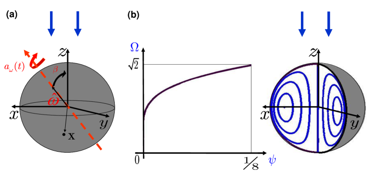
Figure 1: (a) Droplet in the perturbed case (with unsteady rigid body rotation); (b) Streamlines within the droplet for the base (integrable) flow (without rigid body rotation). The motion on each streamline has a frequency $\Omega\left(\psi\right)$ given by Eq. (4).

2.3 Perturbed flow

The perturbed flow is defined by $0<\varepsilon\ll 1$, with the integrals of motion $\psi$ and satisfying

$$\dot{\psi}=-2a_{\omega}(t)\omega_{x}\psi\sin\phi G\left(\psi,\chi\right),~{}~{}~{}~{}\dot{\phi}=a_{\omega}(t)\omega_{z}-a_{\omega}(t)\omega_{x}\cos\phi G\left(\psi,\chi\right),$$ (5)

where $G(\psi,\chi)=z/(x^{2}+y^{2})$ is a $2\pi$ periodic function of $\chi$, with zero average. The time evolution of $\chi$, on the other hand, satisfies the equation

$$\dot{\chi}=\Omega(\psi)+a_{\omega}(t)H(\psi,\phi,\chi),$$

where $H$ is a $2\pi$ periodic function of $\chi$. The perturbed system is characterized by two time scales, a fast one related to the evolution of $\chi$ and a slow one linked to both $\psi$ and $\phi$. As we see below, chaotic advection can be obtained by exploring resonance phenomena between the frequency $\Omega$ of the unperturbed flow (integral case) and the forcing frequency $\omega$.
From a dynamical systems viewpoint, the flow $\bm{V}(\bm{X},t)$ is the superimposition of the integrable flow $\bm{V}_{0}(\bm{X})$ and a small time-dependent perturbation $a_{\omega}(t)\hat{\bm{\omega}}\times\bm{X}$, as given in Eq. (1). Since the unperturbed flow has two invariants, the trajectories of this integrable dynamics are all periodic orbits. Most periodic orbits, however, are expected to break under the influence of a generic time-dependent perturbation with arbitrarily small amplitude, thus possibly leading to chaotic mixing properties. As well-known, the trajectories of an integrable system with only one invariant [36] are two-dimensional tori. Perturbing such an integrable system leads to poor mixing properties since two-dimensional tori (which are robust to small perturbations) act as barriers to chaotic diffusion. As in our previous work [29], the goal of this paper is the generation of three-dimensional chaotic mixing regions of a given size and at specific locations. The strategy we adopt consists of bringing a family of unperturbed tori $\left\{\Gamma_{\psi_{n}}\right\}_{n\in\mathbb{N}^{*}}$ into resonance with the perturbation $a_{\omega}(t)$ by adjusting the frequency $\omega$ in order to satisfy the resonance condition:

$$n\Omega\left(\psi_{n}\right)=\omega.$$ (6)

The notation $CMR_{n}$ is then used to denote the chaotic mixing region created around the torus $\Gamma_{\psi_{n}}$.

We seek to control the mixing by varying the three parameters of the rotation, i.e., its amplitude $\varepsilon$, its frequency $\omega$ and its orientation $\alpha$. Note that the effects of the amplitude and frequency have been studied for a fixed value of $\alpha$ [29].

The effect of a rotation is studied, with an amplitude such that $\varepsilon\ll 1$, with $\varepsilon=0$ at which chaotic mixing is inexistent and $\varepsilon=\varepsilon_{max}$ at which mixing is maximum. In addition, we limit our study to the range $0\leq\omega\leq\sqrt{2}$ which includes the frequencies $\Omega$ of all tori within the droplet. Notice that $\Omega=0$ on the boundary of the droplet and $\Omega=\sqrt{2}$ as the torus approaches the elliptic fixed point. Furthermore, due to the symmetry of Eqs. (2.1), (2) and (3) and without loss of generality, we restrict our study to $0\leq\alpha\leq\pi/2$.

3 Numerical results

3.1 Controlling the location of the chaotic mixing region

In this section, we recall our previous findings on the effect of the amplitude and frequency of the rotation for the orientation $\alpha=\pi/4$, as the influence of the orientation $\alpha$ on these results is studied below.
Figures 2, 3 and  4 display the Liouvillian sections of the perturbed flow, which consist of two-dimensional projections of time-periodic three-dimensional flows by a combination of a stroboscopic map and a plane section. Specifically, the Liouvillian sections considered here are the intersections of the trajectories with the plane $y=0$ at every period $2\pi/\omega$.
Figure 2 shows that the perturbation $a_{\omega}(t)$ creates two non-negligible three-dimensional chaotic mixing regions: one around the torus having the frequency $\omega$ denoted by $CMR_{1}$ and another one $CMR_{n>1}$ around the pole-to-pole axis and near the drop boundary. The latter region contains all tori having a frequency $\omega/n$ with $n>1$.
In Fig. 2, we clearly see that the location of $CMR_{1}$ varies with the value of $\omega$ according to Eq. (6). It is important to note that $CMR_{n>1}$ remains around the pole-to-pole axis and drop boundary due to the nearly vertical part of the curve $\Omega(\psi)$ close to $\psi=0$ (see Fig. 1).
For small values of $\omega$, all resonances are located near the pole-to-pole heteroclinic connections (at $\psi=0$, near the $z-$axis and near the surface of the droplet, see Fig. 2). For larger $\omega$ values, $CMR_{1}$ separates from the chaotic region located close to the heteroclinic orbits and penetrates deeper into the droplet. In the interval $0<\omega<\sqrt{2}$, $CMR_{1}$ is the largest chaotic region, followed by $CMR_{n>1}$ . As $\omega$ is increased further, $CMR_{1}$ moves toward the location of the central elliptic fixed point by following the location of the resonant torus with the frequency $\omega$.

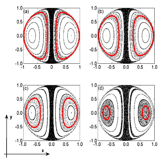
Figure 2: Liouvillian sections for the rotation frequencies $\omega=0.95,1.1,1.25,1.40$ (a-d), amplitude $\varepsilon=0.05$ and orientation $\alpha=\pi/4$. The (red) line inside the chaotic mixing region $CMR_{1}$ is the torus $\Gamma_{\Omega^{-1}(\omega)}$.

3.1.1 Controlling the size of the chaotic mixing region

In this section, we analyze the size of the two main chaotic mixing regions, i.e., $CMR_{1}$ and $CMR_{n>1}$ as the three parameters $\varepsilon$, $\omega$ and $\alpha$ vary. In order to quantify the size, we use the fact that for a trajectory starting at $\psi=\psi_{0}$ the adiabatic invariant varies between $\psi^{-}\left(\psi_{0};\varepsilon,\alpha,\omega\right)$ and $\psi^{+}\left(\psi_{0};\varepsilon,\alpha,\omega\right)$. It then follows that the width $\Delta\psi=\psi^{+}\left(\psi_{0};\varepsilon,\alpha,\omega\right)-\psi^{-}\left(\psi_{0};\varepsilon,\alpha,\omega\right)$ is large close to the resonance but decreases as one goes away from it. This quantity thus seems to be a good candidate to quantitatively estimate the size of $CMR_{1}$ and $CMR_{n>1}$.
As explained above, the location of $CMR_{1}$ is mostly determined by the rotation frequency $\omega$ (while $CMR_{n>1}$ is always located in the neighborhood of the heteroclinic orbits). However, the size of $CMR_{1}$ and $CMR_{n>1}$ can be varied by adjusting the rotation amplitude $\varepsilon$ and orientation $\alpha$. This is illustrated in Fig. 3 which shows that the size of these chaotic mixing regions clearly increases with the amplitude of the perturbation. It is also interesting to note that around $\varepsilon=\varepsilon_{max}\approx 0.20$, the two regions join and invade the entire drop. At that point, complete chaotic mixing is obtained. The size of $CMR_{1}$ as a function of the frequency $\omega$ is shown in Fig. 5 (middle panel). From this figure it is clear that for each value of $\varepsilon$ the size reaches a maximum for a certain value $\omega^{m}\left(\varepsilon\right)$ of the forcing frequency.

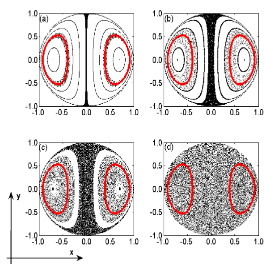
Figure 3: (Color on line) Liouvillian sections for the rotation frequency $\omega=1.25$, amplitudes $\varepsilon=0.01,0.05,0.10,0.20$ (a-d) and orientation $\alpha=\pi/4$. The (red) line inside the chaotic mixing region $CMR_{1}$ is the torus $\Gamma_{\Omega^{-1}(\omega)}$.

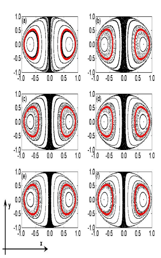
Figure 4: Liouvillian sections for the rotation frequency $\omega=1.25$, amplitude $\varepsilon=0.05$ and orientations $\alpha=\pi/64,\pi/8,5\pi/16,3\pi/8,7\pi/16$ (a-f). The (red) line inside the chaotic mixing region $CMR_{1}$ is the torus $\Gamma_{\Omega^{-1}(\omega)}$.

The effect of the orientation $\alpha$ on the size of $CMR_{1}$ is interesting. Indeed two distinguishable behaviors can be observed, one in which $\alpha$ hardly affects the size and another one in which $\alpha$ has a strong influence. These conclusions can be drawn from the lower panel of Fig. 5, where the size of the chaotic mixing region $CMR_{1}$ is displayed as a function of $\alpha$. It is indeed clear that when $\alpha$ is not close to the limit values, i.e., $0$ and $\pi/2$, the size stays practically constant, but when $\alpha$ gets close to $0$ and $\pi/2$, it decreases significantly. Such observation is confirmed by looking at the Liouvillian sections in Fig. 4. In the first two panels, we see a very small change in size while the size of the chaotic mixing regions starts decreasing in the third panel and shrinks drastically in the fourth panel. Being aware of the dependence of the size of $CMR_{1}$ with respect to the orientation of the rotation $\alpha$ can be handy in practice in order to control the size of the mixing region.
Indeed, in some applications where one is faced with the challenge of precisely controlling the size of the mixing zone despite uncontrollable, yet relatively small, fluctuations of $\alpha$, setting $\alpha$ far away from the limit values $0$ and $\pi/2$ and manipulating the chaotic zone size through the parameter $\varepsilon$ should be desirable. In other, perhaps more gentle, applications where increasing the amplitude of the rotation may not be possible (e.g., in biomedical handling where biological particles need to be handled with care), fixing $\varepsilon$ while tuning the size of the mixing by varying $\alpha$ around the limit values $\alpha=0$ or $\alpha=\pi/2$ could be the solution. One should notice, however, that at the critical orientation $\alpha=\pi/2$ no chaotic mixing occurs and $\psi$ is conserved.

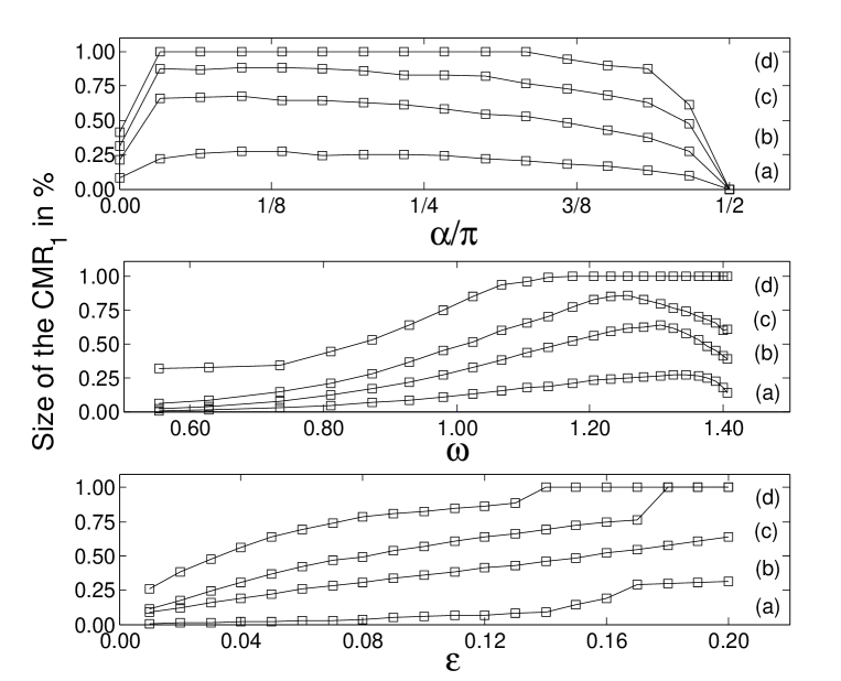
Figure 5: Size of the chaotic mixing region. Upper panel: Normalized size $\Delta\psi$ vs. orientation $\alpha$ for the amplitudes $\varepsilon=0.01,0.05,0.10,0.20$ (a-d) and a frequency $\omega=1.25$; Middle panel: Normalized size $\Delta\psi$ vs. frequency $\omega$ for the amplitudes $\varepsilon=0.01,0.05,0.10,0.20$ (a-d) and an orientation $\alpha=\pi/4$ ; Lower panel: Normalized size $\Delta\psi$ vs. amplitude $\varepsilon$ for the frequencies $\omega=0.55,0.93,1.28,1.41$ (a-d) and an orientation $\alpha=\pi/4$.

4 Design of an experimental set up

In this work, the flow within a drop was produced by the superimposition of an external steady translation and an unsteady rigid body rotation. The drop steady translating motion along the channel could simply be produced by means of a constant pressure gradient, exploring the buoyancy force in the case of a vertical column or using traveling wave dielectrophoresis in a microchannel [34]. The unsteady rigid rotation could be realized by applying an electric field that exerts a torque on the droplet as it is the case with traveling wave dielectrophoresis which generates both a force and a torque (although both are not independent) [34]. Another possibility is by using the so-called “electrorotation” phenomenon which creates a torque [35]. Electrorotation stands for the spinning of an electrically polarized particle while the latter is subjected to a “rotating” electric field, that is an ac electric field generated by voltages which are out of phase of one another.
A possible design based on the latter phenomenon is proposed in Fig. 6. This device consists of a vertical square column/channel with electrodes embedded within its four walls creating a rotating electric field due to the phase difference between the voltages applied to adjacent electrodes in the same plane. It is known that such a four-pole electrode setting would generate a torque on the droplet trapped in the middle of the channel, with the torque strength being proportional to the square of the intensity of the electric field. The periodicity in the angular velocity is then obtained by imposing a phase difference to the voltages applied between two four-pole electrode settings in two different $x-y-$planes $P_{i}$ and $P_{i+1}$, so that a torque around the $z-$direction acts on the drop as it passes through $P_{i}$ and a torque around the $z-$direction acts on the drop as it passes through $P_{i+1}$. Although such a device would not produce exactly the one harmonic angular velocity profile described in Eq. (2.1), our previous study [37] has shown that the strategy is robust with respect to the specific time dependent function used for the rotation. Specifically, results were very similar when the sinusoidal rotation was replaced by a periodic triangular function. Finally, the control of the orientation of the rotation axis could be realized by a series of electrodes lying within inclined planes along the length of the channel (see Fig. 6).

Figure 6: Sketch of a possible design for the experimental apparatus showing (a) the square channel/column with a series of out-of-phase embedded electrodes, where $\omega_{e}$ and $V_{e}$ stand for the frequency and amplitude of the voltage applied to the electrodes; (b) the four-pole electrode setting generating a torque in the $z-$direction, i.e., in the direction of translation, $\tau>0$; (c) the four-pole electrode in a consecutive plane setting generating a torque in the $z-$direction, i.e. in the direction opposed to the direction of translation, $\tau<0$.

5 Conclusions

In this work, we have further studied the generation of chaotic mixing within a translating droplet by adding a perturbation in the form of an oscillatory rigid body rotation. As previously [29], the frequency of the latter was selected in order to create resonances with the natural frequencies of the system, namely the frequencies of the various tori embedded within the drop. A particularly interesting feature of the perturbed system lies in the fact that both the size and the location of the mixing region can be varied by adjusting the frequency and amplitude of the rigid body rotation.
In this work, we have added a third parameter, namely the orientation of the rotation axis. It was found that the latter can influence the size of the chaotic mixing regions and that the size can significantly decrease when the angle between the rotation axis and the direction of translation approaches either $0$ or $\pi/2$. Away from these two limit values, the size of the chaotic mixing region is maximal and the particular value of the angle has only a minor effect.
A possible design for an experimental set up capable of guiding a drop in a controlled fashion by varying the amplitude, frequency and orientation of the rotation was also proposed.

References

- [1] H. Aref, The development of chaotic advection, Phys. Fluids 14, (2002) 1315-1325.
- [2] P. Castiglione, A. Mazzino, P. Muratore-Ginanneschi and A. Vulpiani, On strong anomalous diffusion, Physica D 134, (1999) 75-93.
- [3] G. Mathew, I. Mezic, S. Grivopoulos, U. Vaidya and L. Petzold, Optimal control of mixing in Stokes fluid flows, J. Fluid Mech. 580, (2006) 261-281.
- [4] T.H. Solomon and J.P. Gollub, Chaotic particle transport in time-dependent Rayleigh-Bénard convection, Phys. Rev. A 38, (1988) 6280-6286.
- [5] T.H. Solomon and J.P. Gollub, Passive transport in steady Rayleigh-Bénard convection, Phys. Fluids 31, (1988) 1372-1379.
- [6] M.S. Paoletti, C.R. Nugent and T.H. Solomon, Synchronization of Oscillating Reactions in an Extended Fluid System, Phys. Rev. Lett. 96, (2006) 124101.1-124101.4.
- [7] A.M. Mancho, D. Small and S. Wiggins, A tutorial on dynamical systems concepts applied to Lagrangian transport in oceanic flows defined as finite time data sets: Theoretical and computational issues, Phys. Rep. 437, (2006) 55-124.
- [8] A. Crisanti, M. Falcioni, G. Paladin and A. Vulpiani, Lagrangian chaos - Transport, mixing and diffusion in fluids, Rivista Del Nuovo Cimento 14, (1991) 1-80.
- [9] K. Bajer and H.K. Moffatt, On a class of steady confined Stokes flows with chaotic streamlines, J. Fluid Mech. 212, (1990) 337-363.
- [10] D. Kroujiline and H.A. Stone, Chaotic streamlines in steady bounded three-dimensional Stokes flows, Physica D 130, (1999) 105-132.
- [11] H. Song, J.D. Tice and R.F. Ismagilov, A Microfluidic System for Controlling Reaction Networks in Time, Angew. Chem. Int. Edit. 42, (2003) 768-772.
- [12] M.R. Bringer et al., Microfluidic systems for chemical kinetics that rely on chaotic mixing in droplets, Philos. Transact. A Math. Phys. Eng. Sci. 362, (2004) 1087-1104.
- [13] M.H. Oddy, J.G. Santiago, J.C. Mikkelsen, Electrokinetic Instability Micromixing, Anal. Chem. 73, (2001) 5822-5832.
- [14] H.H. Bau, J. Zhong and M. Yi, A minute magneto hydrodynamic (MHD) mixer, Sens. Actuators B 79, (2001) 207-215.
- [15] A. Ould El Moctar, N. Aubry and J. Batton, Electro-hydrodynamic micro-fluidic mixer, Lab Chip 3, (2003) 273-280.
- [16] I.K. Glasgow and N. Aubry, Enhancement of microfluidic mixing using time pulsing, Lab Chip 3, (2003) 114-120.
- [17] I.K. Glasgow, J. Batton and N. Aubry, Electroosmotic mixing in microchannels, Lab Chip 4, (2004) 558-562.
- [18] A. Goullet, I.K. Glasgow and N. Aubry, Effects of microchannel geometry on pulsed flow mixing, Mech. Res. Commun. 33, (2006) 739-746.
- [19] X. Niu and Y-K. Lee, Efficient spatial-temporal chaotic mixing in microchannels, J. Micromech. Microeng. 13, (2003) 454-462.
- [20] F. Bottausci et al., Mixing in the shear superposition micromixer: three-dimensional analysis, Phil. Trans. Royal Soc. A 362, (2004) 1001-1018.
- [21] M.A. Stremler, F.R. Haselton and H. Aref, Designing for chaos: applications of chaotic advection at the microscale, Phil. Trans. Royal Soc. A 362, (2004) 1019-1036.
- [22] S.M. Lee, D.J. Im and I.S. Kang, Circulating flows inside a droplet under time-periodic nonuniform electric fields, Phys. Fluids 12, (2000) 1899-1910.
- [23] T. Ward and G.M. Homsy, Electrohydrodynamically driven chaotic mixing in a. translating droplet, Phys. Fluids 13, (2001) 3521-3525.
- [24] R.O. Grigoriev, Chaotic mixing in thermocapillary-driven microdroplets, Phys. Fluids 17, (2005) 033601.1-033601.8.
- [25] X.M. Xu and G.M. Homsy, Three-dimensional chaotic mixing inside droplets driven by a transient electric field, Phys. Fluids 19, (2007) 013102.1-013102.11.
- [26] D.L. Vainchtein, J. Widloski and R. Grigoriev, Resonant chaotic mixing in a cellular flow, Phys. Rev. Lett. 99, (2007) 094501.1-094501.4.
- [27] T. Ward and G.M. Homsy, Electrohydrodynamically driven chaotic mixing in a translating droplet part II: Experiments, Phys. Fluids 15, (2003) 2987-2994.
- [28] R.O. Grigoriev, M.F. Schatz and V. Sharma, Optically controlled mixing in microdroplets, Lab Chip 6, (2006) 1369-1372.
- [29] R. Chabreyrie et al., Tailored mixing inside a translating droplet, Phys. Rev. E 77, (2008) 036314.1-036314.4.
- [30] D. Vainchtein, A. Vasiliev and A. Neishtadt, Adiabatic chaos in a two-dimensional mapping, Chaos 6, (1996) 514-518.
- [31] D. Vainchtein, A. Neishtadt and I. Mezić, On passage through resonances in volume-preserving systems, Chaos 16, (2006) 043123.1-043123.11.
- [32] R. Lima and M. Pettini, Suppression of chaos by resonant parametric perturbations, Phys. Rev. A 41, (1990) 726-733.
- [33] J.H.E. Cartwright, M. Feingold and O. Piro, Chaotic advection in three-dimensional unsteady incompressible laminar flow, J. Fluid Mech. 316, (1996) 259-284.
- [34] N. Aubry and P. Singh, Influence of particle-particle interactions and particle rotational motions in traveling wave dielectrophoresis, Electrophoresis 27, (2006) 703-715.
- [35] W.M. Arnold, U. Zimmermann, Electro-rotation: development of a technique for dielectric measurements on individual cells and particles, J. Electrostat. 21, (1988) 151-191.
- [36] M. Feingold, L.P. Kadanoff and O. Piro, Passive scalars, three-dimensional volume-preserving maps, and chaos, J. Stat. Phys. 50, (1988) 529-565.
- [37] R. Chabreyrie et al., Tuning mixing within a droplet for digital microfluidics, Mech. Res. Commun. 36, (2008) 130-136.