Dust amorphization in protoplanetary disks

Abstract

Aims. High-energy irradiation of the circumstellar material might impact the structure and the composition of a protoplanetary disk and hence the process of planet formation. In this paper, we present a study on the possible influence of the stellar irradiation, indicated by X-ray emission, on the crystalline structure of the circumstellar dust.

Methods. The dust crystallinity is measured for 42 class II T Tauri stars in the Taurus star-forming region using a decomposition fit of the 10 $\mu$m silicate feature, measured with the Spitzer IRS instrument. Since the sample includes objects with disks of various evolutionary stages, we further confine the target selection, using the age of the objects as a selection parameter.

Results. We correlate the X-ray luminosity and the X-ray hardness of the central object with the crystalline mass fraction of the circumstellar dust and find a significant anti-correlation for 20 objects within an age range of approx. 1 to 4.5 Myr. We postulate that X-rays represent the stellar activity and consequently the energetic ions of the stellar winds which interact with the circumstellar disk. We show that the fluxes around 1 AU and ion energies of the present solar wind are sufficient to amorphize the upper layer of dust grains very efficiently, leading to an observable reduction of the crystalline mass fraction of the circumstellar, sub-micron sized dust. This effect could also erase other relations between crystallinity and disk/star parameters such as age or spectral type.

1 Introduction

The evolution of the dust in a protoplanetary disk is one of the key subjects in the overall research on mechanisms of planet formation. As we now know, dust in young circumstellar disks differs significantly from the dust in the interstellar medium (ISM). There is evidence for grain growth from the typical ISM and sedimentation in the vertical direction (or dust settling) of a disk (see various references such as Rodmann et al. 2006, Sicilia-Aguilar et al. 2007, Furlan et al. 2006). While the dust grains in the ISM and in molecular clouds are amorphous, protoplanetary disks contain an increased content of crystalline silicates (Bouwman et al. 2008). This transition of the dust grain structure during the star-forming process is poorly understood and could be important in the later scenario of planet formation.

However, as many authors have pointed out (e.g. Watson et al. 2009, Sicilia-Aguilar et al. 2007, van Boekel et al. 2005, Schegerer et al. 2006), no definitive connection have been found so far between the properties of the disk or of the central object and the crystalline mass fraction of the dust disk. From the point of view of standard dust processing scenarios for protoplanetary disks, this conclusion is surprising. We expect the crystallization of the dust grains to occur due to thermal annealing or evaporation and recondensation processes either close to the star or within accretion shocks (Henning 2008). Radial mixing may transport the crystalline grains to more distant regions (e.g., Gail 2004). Therefore, we expect an evolutionary trend for the crystalline mass fraction and/or correlations with stellar parameters such as the bolometric luminosity, the photospheric temperature, the accretion rate or the disk/star mass ratio. The fact that no such relation has been found raises the question on alternative mechanisms, controlling the process of crystallization. Kessler-Silacci et al. (2006) and Watson et al. (2009) suggested that the crystallizing process might be dominated by the impact of X-ray irradiation which destroys the crystalline structure of the dust grains.

Young stars are very strong sources of X-rays. A typical T Tauri star emits between $10^{29}$ and $10^{31}$ erg s^-1 in the soft ($0.1-10$ keV) X-ray band, i.e., $2-4$ orders of magnitude more than the Sun (see Güdel 2004 for a review of stellar X-ray radiation). The radiation is thought to be mostly coronal, originating from hot ($1-20$ million K), magnetically trapped plasma above the stellar photosphere, in analogy to the solar coronal X-ray radiation.

There is little doubt that X-rays have some impact on the gas and dust in circumstellar disks, at least relatively close to the star and at the disk surface. For example, Igea & Glassgold (1999), Glassgold et al. (2004) or Ercolano et al. (2008) computed detailed models for radial distances between 0.5-10 AU that indicate efficient ionization of circumstellar disks by X-rays and also heating of the gaseous surface layers to several thousands of Kelvin. Complicated chemical networks are a consequence (e.g., Semenov et al. 2004 or Ilgner & Nelson 2006). A direct evidence for these processes is suggested from the presence of strong line radiation of [Ne ii] at 12.8 $\mu$m detected by Spitzer in many T Tauri stars (e.g., Pascucci et al. 2007, Herczeg et al. 2007 or Lahuis et al. 2007) which in some cases may be triggered by shocks (van Boekel et al. 2009). This transition requires ionization and heating of the ambient gas to several 1000 K (Glassgold et al. 2007).

Magnetic energy release events, so-called flares, occurring in the same stellar coronae can increase the X-ray output up to hundreds of times, but as we know from solar observations, such events are also accompanied by high-energy electrons, protons and ions ejected from the Sun. Feigelson et al. (2002) speculated that the expected elevated proton flux around T Tauri stars leads to isotopic anomalies in solids in the accretion disk, as suggested from measurements of meteoritic composition for our early solar system (Caffe et al. 1987).

The destructive impact of high-energy irradiation on crystalline structures by ions has been demonstrated in laboratory measurements by, e.g., Jäger et al. (2003), Bringa et al. (2007), Demyk et al. (2001), Carrez et al. (2002), mainly for low energetic cosmic rays ($E\ga$50 keV) but rarely also for lower energies typical of stellar winds.

In this study we look in particular for correlations between the crystalline mass fraction and stellar properties related to X-ray emission by deriving these parameters for T Tauri stars in the Taurus-Auriga star formation region. We present in Sect. 2 the target sample and some aspects of the data reduction, describe in Sect. 3 the methodology of measuring the crystalline mass fraction based on decomposition fits to the 10 $\mu$m silicate feature, present the derived values in Sect. 4 and bring them into context with X-ray parameters in Sect. 5. Our conclusions are presented in Sect. 6.

2 Data sample and data reduction

We use the sample of objects in common to two recent surveys of the Taurus-Auriga star-forming region. The first survey was obtained by the Spitzer InfraRed Spectrograph (IRS) and was published previously by Furlan et al. (2006) and further analyzed by Watson et al. (2009). The second survey was performed in the X-ray range with XMM-Newton as described by Güdel et al. (2007). While the former survey provides information on the dust properties of the circumstellar disks, the latter allows the investigation of stellar X-rays. We focus only on the disk surrounded (Class II, as listed in Güdel et al. 2007) T Tauri stars which appear in both surveys and show significant emission in the 10 $\mu$m silicate feature. Table 1 provides an overview of the objects used for this study and their properties derived in the framework of the XMM-Newton survey.

Table 1: Object sample and stellar properties (X-ray luminosity $L_{\mathrm{X}}$ , hardness $H$, spectral type, photosphere temperature $T_{\star}$ and stellar age) published in Güdel et al. (2007)

Name	$L_{\mathrm{X}}$	$H$	Spect	$T_{\star}$[0.0pt]	Age
	[1030 erg/s]			[K]	[My]
04187+1927	0.91	$0.57$	M0	3850	$-$
04303+2240	4.99	$0.76$	M0.5	3700	$0.5$
04385+2550	0.40	$2.26$	M0	3850	$-$
AA Tau	1.24	$1.98$	K7	4060	$2.4$
BP Tau	1.36	$0.68$	K7	4060	$1.9$
CI Tau	0.19	$1.62$	K7	4060	$2.2$
CoKu Tau/3	5.83	$0.68$	M1	3705	$0.9$
CW Tau	2.84	$-$	K3	4730	$7.0$
CY Tau	0.13	$0.46$	M1.5	3632	$1.5$
CZ Tau	0.42	$0.43$	M3	3415	$2.1$
DD Tau	0.09	$2.55$	M3	3412	$4.5$
DK Tau	0.91	$0.75$	K7	4060	$1.3$
DN Tau	1.15	$1.01$	M0	3850	$1.1$
FM Tau	0.53	$1.34$	M0	3850	$2.8$
FO Tau	0.06	$1.13$	M2	3556	$1.5$
FQ Tau	0.12	$0.36$	M3	3416	$2.8$
FS Tau	3.21	$0.73$	M0	3876	$3.1$
FV Tau	0.53	$0.50$	K5	4395	$4.8$
FX Tau	0.50	$0.52$	M1	3720	$0.9$
FZ Tau	0.64	$0.87$	M0	3850	$1.1$
GH Tau	0.11	$0.98$	M1.5	3631	$2.0$
GI Tau	0.83	$0.90$	K7	4060	$1.8$
GK Tau	1.47	$0.96$	K7	4060	$1.2$
GN Tau	0.78	$1.18$	M2.5	3488	$1.0$
GO Tau	0.25	$1.09$	M0	3850	$3.8$
Haro 6-13	0.80	$1.99$	M0	3800	$0.6$
Haro 6-28	0.25	$0.75$	M2	3556	$10$
HK Tau	0.08	$4.19$	M0.5	3778	$1.8$
HO Tau	0.05	$0.08$	M0.5	3778	$9.1$
HP Tau	2.54	$1.02$	K3	4730	$6.9$
IQ Tau	0.41	$1.17$	M0.5	3778	$1.1$
IS Tau	0.66	$0.48$	K7	3999	$4.2$
IT Tau	6.47	$2.05$	K2	4900	$4.8$
MHO-3	0.46	$1.26$	K7	4060	$2$
RY Tau	5.50	$1.41$	K1	5080	$2.1$
UZ Tau/e	0.89	$0.49$	M1	3705	$2.3$
V410 Anon 13	0.01	$0.68$	M5.8	3024	$-$
V710 Tau	1.37	$0.76$	M0.5	3778	$1.7$
V773 Tau	9.46	$1.08$	K2	4898	$6.4$
V807 Tau	1.05	$0.52$	K7	3999	$1.5$
V955 Tau	1.62	$0.46$	K5	4395	$6.7$
XZ Tau	0.96	$1.05$	M2	3561	$4.6$

The Spitzer IRS data were obtained during the observing campaigns 3, 4 and 12 using mainly the low resolution channel. Two exposures per object were obtained in different nod positions allowing the subtraction of the background by subtracting the two spectra, $F_{\nu,1}(\lambda)$ and $F_{\nu,2}(\lambda)$, from each other. The fluxes are then averaged over the two observations and the difference of the two spectra $d(\lambda)=F_{\nu,1}(\lambda)-F_{\nu,2}(\lambda)$ is used to estimate the uncertainties of the observation. However, $d(\lambda)$ is not the correct error estimator; although it does contain the errors due to statistical fluctuations, it is also sensitive to systematic effects such as the truncation of the flux by misalignment of one of the two observations. Therefore, we make a first order correction of the uncertainty by subtracting the averaged difference

$$\tilde{d}(\lambda)=d(\lambda)-\langle d(\lambda)\rangle_{\lambda\in[7,14\mu\mathrm{m}]}$$ (1)

where the average is taken over the wavelength range which is relevant for the fit procedure used later for the 10 $\mu$m-silicate feature. This correction brings $\tilde{d}(\lambda)$ closer to the truly random noise contributions. However, $\tilde{d}(\lambda)$ can underestimate the purely statistical fluctuations (noise) by chance at various wavelengths. But assuming that the noise remains similar across a narrow window in wavelength, we can obtain its statistical value from the fluctuations of $\tilde{d}(\lambda)$ itself. We use $N=11$ data points around each wavelength bin $\lambda_{i}$ to derive the measurement uncertainties $\sigma$ by computing a geometrical sum of their average and standard deviation of the systematic differences $\tilde{d}(\lambda)$:

$$\sigma^{2}(\lambda_{i}) = \sum_{j\in\mathbb{A}}{\frac{(\tilde{d}(\lambda_{j})-\langle\tilde{d}(\lambda_{k})\rangle_{k\in\mathbb{A}})^{2}}{N-1}}+\left(\langle\tilde{d}(\lambda_{k})\rangle_{k\in\mathbb{A}}\right)^{2}$$ (2)

$$\textrm{with }\mathbb{A}=[i-5,i+5]$$

The X-ray data were obtained from the XMM-Newton Extended Survey of the Taurus Molecular Cloud (XEST) which consisted of 28 exposures in total, spread over the whole Taurus region. Parameters used for this work are the stellar X-ray luminosity $L_{\mathrm{X}}$ and further, we defined the hardness $H$ of the stellar X-ray emission as the ratio between the hard and soft luminosity components. This allows to measure the relative contribution of different energy bands to the X-ray radiation; the hard and soft bands comprise the $1-10$ keV and the $0.3-1$ keV ranges, respectively:

$$H=\frac{L_{\mathrm{X}}(1\leavevmode\nobreak\ \mathrm{keV}<E<10\leavevmode\nobreak\ \mathrm{keV})}{L_{\mathrm{X}}(0.3\leavevmode\nobreak\ \mathrm{keV}<E<1\leavevmode\nobreak\ \mathrm{keV})}\quad.$$ (3)

As a few objects such as DH Tau showed excessive emission during the observation (as described by Telleschi et al. 2007), their value for $L_{\mathrm{X}}$ does not correspond to the actual averaged luminosity which is the parameter of interest for the present study. Therefore, these objects have been discarded from our sample.

The last column of Table 1 lists the stellar age (from Güdel et al. 2007). These values were derived from $T_{\rm eff}$ and $L_{*}$ as given in the literature and provide best-estimate values for which systematic uncertainties are difficult to provide. Although Güdel et al. indicated conservative age uncertainties (based on a variety of literature values for $T_{\rm eff}$ and $L_{*}$) of factors of 2–3, these are extreme values, and most ages are - within the framework of one set of evolutionary tracks (Siess et al. 2000 in Güdel et al. 2007) - much more narrowly confined. As for the original parameters used for age determination, $T_{\rm eff}$ and $L_{*}$, White & Ghez (2001) (used in the XEST study) estimate uncertainties in $L_{*}$ of 0.1–0.3 dex for their sample. Hartigan & Kenyon (2003) (also used in the XEST study) estimate errors in $L_{*}$ from the disagreement of ages between components of binaries, amounting to typically 0.1–0.2 dex. A similar uncertainty (0.11 dex) for $L_{*}$ has also been given by Kenyon & Hartmann (1995). A scatter of 0.2-0.3 dex is furthermore found when comparing values from various authors. We thus conclude that most of our ages (primarily determined by $L_{*}$ and much less by $T_{\rm eff}$) are accurate to within a factor of 1.5–2.

The range of the stellar ages spreads from 0.5 to 10 Myr. Although our sample consists of Class II T Tauri stars only, this wide range indicates that the selected objects can be categorized into three evolutionary groups: Very young objects ($\lesssim$1 Myr) which are likely to be in a transitional phase from embedded to disk-only geometries; typical Class II objects with a pure disk geometry; and older objects ($\gtrsim$5 Myr) which are more mature Class II sources and are likely to have changed characteristics compared to their younger counterparts. These groups are not separated sharply given the age uncertainties. Also, we note that age is not the only parameter determining the evolutionary state of the disk. Therefore we continue to study the full sample and will investigate the object selection later in this paper (see Sect. 5.2).

3 The decomposition of the 10 $\mu$m silicate feature

3.1 Modeling of the Emission Profile

Our model describes the total observable flux with three components based on the two-layer temperature distribution (TLTD) method introduced by Juhasz et al. (2009): The emission from the stellar photosphere, a continuum emission from the opaque disk midplane and emission from the optically thin disk atmosphere consisting of thermal emission from dust grains of different mineralogy and temperature. The atmosphere is transparent with respect to the continuum emission of the disk midplane. Figure 1 shows a sketch of the disk model.

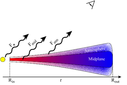
Figure 1: Circumstellar disk model describing the observable total flux which is a superposition of the stellar light, $F_{\star}$, the continuum emission from the disk midplane, $F_{\mathrm{mid}}$, and the emission from the optically thin disk atmosphere, $F_{\mathrm{atm}}$.

The total observable flux is given by

$$F_{\nu,\mathrm{tot}}=F_{\nu,\star}+F_{\nu,\mathrm{mid}}+F_{\nu,\mathrm{atm}}\quad.$$ (4)

We describe the flux of the stellar photosphere approximately with the emission of a blackbody with a temperature $T_{\star}$:

$$F_{\nu,\star}=C_{\star}\frac{2h\nu^{3}}{c^{2}}\frac{1}{e^{h\nu/kT_{\star}}-1}\equiv C_{\star}\cdot B_{\nu}(T_{\star})\quad.$$ (5)

$C_{\star}$ is the normalization factor used for the later fit and $B_{\nu}(T)$ defines the Planck function at temperature $T$. To model the flux from the midplane and the atmosphere of the disk, we set up two simple continuum emission profiles, one of which we use directly for the midplane while the other is multiplied by dust grain absorption coefficients $\kappa_{\nu,i}$ for modeling the flux from the atmosphere. These two continuum emission profiles are constructed as a superposition of blackbody spectra taking a radial temperature distribution $T(r)$ and geometrical aspects of the disk into account, assuming axisymmetry. Hence, the fluxes can be written as

$$F_{\nu,\mathrm{mid}}=\tilde{C_{0}} \cdot \int_{R_{\mathrm{mid,in}}}^{R_{\mathrm{mid,out}}}B_{\nu}(T_{\mathrm{mid}}(r))\cdot r\cdot\textrm{d}r$$ (6)

$$F_{\nu,\mathrm{atm}}=\sum_{i=1}^{N}\tilde{C_{i}}\cdot\kappa_{\nu,i} \cdot \int_{R_{\mathrm{atm,in}}}^{R_{\mathrm{atm,out}}}B_{\nu}(T_{\mathrm{atm}}(r))\cdot r\cdot\textrm{d}r$$ (7)

where $r$ is the radial distance to the central object, $R_{\mathrm{atm/mid,in/out}}$ the inner and outer radii of the disk midplane and atmosphere, respectively (see Fig. 1), $\tilde{C_{i}}$ are the normalization factors of the $N$ dust species $i$ (in our case we use $N=10$, see Sect. 3.2) and $\tilde{C_{0}}$ of the disk midplane emission, respectively. We assume the temperature distributions to follow a simple power law with

$$\frac{T_{\mathrm{mid}}(r)}{T_{\mathrm{mid,max}}} = \left(\frac{r}{R_{\mathrm{mid,in}}}\right)^{q_{\mathrm{mid}}}$$ (8)

$$\frac{T_{\mathrm{atm}}(r)}{T_{\mathrm{atm,max}}} = \left(\frac{r}{R_{\mathrm{atm,in}}}\right)^{q_{\mathrm{atm}}}$$ (9)

which implies that all grains in the atmosphere or in the disk mid-plane follow the same temperature profile, regardless their size and chemical composition. This allows a substitution of $r$ with $T$ and Eqs. (6) and (7) can be rewritten as

$$F_{\nu,\mathrm{mid}}=\frac{C_{0}}{q_{\mathrm{mid}}} \cdot \int_{T_{\mathrm{mid,max}}}^{T_{\mathrm{mid,min}}}B_{\nu}(T)\cdot T^{(2-q_{\mathrm{mid}})/q_{\mathrm{mid}}}\leavevmode\nobreak\ \textrm{d}T$$ (10)

$$F_{\nu,\mathrm{atm}}=\sum_{i=1}^{N}\frac{C_{i}\cdot\kappa_{\nu,i}}{q_{\mathrm{atm}}} \cdot \int_{T_{\mathrm{atm,max}}}^{T_{\mathrm{atm,min}}}B_{\nu}(T)\cdot T^{(2-q_{\mathrm{atm}})/q_{\mathrm{atm}}}\leavevmode\nobreak\ \textrm{d}T$$ (11)

where $C_{i}$ are the new normalization factors used for the later fit. In this fitting approach, $C_{\star}$,$C_{0}$, $\dots$, $C_{N}$, $q_{\mathrm{mid}}$, $q_{\mathrm{atm}}$, $T_{\star}$, $T_{\mathrm{mid,max}}$, $T_{\mathrm{mid,min}}$, $T_{\mathrm{atm,max}}$ and $T_{\mathrm{atm,min}}$ are fitting parameters. As we are only interested in a wavelength range between $\sim$7 $\mu$m and 14 $\mu$m (see Sect. 5.1 for a discussion), we can eliminate several of these parameters:

• $T_{\star}$ can be derived from the literature. We used the values summarized in Table 1.

• We chose to set $T_{\mathrm{mid,min}}$ and $T_{\mathrm{atm,min}}$ to 10 K to account for the contribution of the cooler region of the disk which is irrelevant for the mid-infrared regime.

• Figure 2 shows the impact of $T_{\mathrm{mid,max}}$ on the shape of the flux function given by Eq. (10) by keeping $q_{\mathrm{mid}}$ constant.

  

  Figure 2: Normalized flux as expressed by Eq. (10) for $q=-0.5$ and $T_{\mathrm{mid,max}}=250$ K, 500 K, $\dots$, 2500 K.

  It is obvious that $T_{\mathrm{mid,max}}$ has no significant influence on the shape of the flux function for values $T_{\mathrm{mid,max}}>1000$ K, which is true for various values of $q_{\mathrm{mid}}$. Further, D’Alessio et al. (1998) showed that the inner disks of classical T Tauri stars (CTTS) reach temperatures around $T_{\mathrm{sub}}=1800-2000$ K due to the dust sublimation. Therefore, we set without loss of generality $T_{\mathrm{mid,max}}=1800$ K. With the same argumentation we set $T_{\mathrm{atm,max}}=1800$ K.

• First trials of fitting simulated spectra showed that the fit is not sensitive to $q_{\mathrm{atm}}$ for any physically meaningful value (e.g., $0\geq q_{\mathrm{atm}}\geq-2$) as the influence on the shape of the flux function in Eq. (11) is fully dominated by the dust emission profile. We therefore set $q_{\mathrm{atm}}=q_{\mathrm{mid}}\equiv q$.

Consequently, the remaining fit parameters are $C_{\star}$, $C_{0}$, $\dots$, $C_{N}$ and $q$. For a given $q$ and more than $N+2$ data points, $C_{\star}$, $C_{0}$, $\dots$, $C_{N}$ can be derived analytically according to a non-negative least-square fit (see e.g. Lawson & Hanson 1974) and further, a unique solution exists. Therefore, we can search efficiently for a global minimum of $\chi^{2}(q)$.

To derive the components $C_{i}$ and $q$ of the fit function and their errors for a given observation, we compute 100 spectra adding Monte-Carlo simulated, normally distributed noise to the original data; the noise distribution is based on the spectral errors of the original data. Each of these spectra is then fitted with a least-square method approach as we take the median values (the distributions tend to be very asymmetric) of the resulting parameters to obtain the final parameters and their errors (1$\sigma$ range of the frequency distribution).

3.2 Emission profiles

We use emission profiles analogous to Schegerer et al. (2006) and Bouwman et al. (2008): For the amorphous silicates we use profiles calculated for homogeneous, compact, and spherical grains applying Mie theory. For the crystalline silicates we use emission profiles calculated for inhomogeneous spheres according to the distribution of hollow spheres (DHS, Min et al. 2005). We start from the complex refractive indices $n_{i}$ for silicate material $i$. The result is the dimensionless absorption efficiency $Q_{i}$, which is used for calculating the mass absorption coefficient $\kappa_{m,i}=Q_{i}\pi a^{2}/(4/3\pi a^{3}\rho)$ where $a$ is the particle radius and $\rho$ the material density. We fit the 10 $\mu$m silicate feature with amorphous silicates with the stoichiometries of olivine (MgFeSiO₄) and pyroxene (MgFe$[$SiO${}_{3}]_{2}$) and the crystalline silicates forsterite (Mg₂SiO₄), enstatite (MgSiO₃) and quartz (SiO₂). Table 2 summarizes the dust species considered here.

Table 2: Dust species used for the decomposition fit of the 10 $\mu$m feature fit.

Name	Stoichiometry	Structure	Reference
Olivine	MgFeSiO4	a	Dorschner et al. 1995
Pyroxene	MgFe$[$SiO${}_{3}]_{2}$	a	Dorschner et al. 1995
Forsterite	Mg2SiO4	c	Servoin & Piriou 1973
Enstatite	MgSiO3	c	Jäger et al. 1998
Quartz	SiO2	c	Spitzer & Kleinman 1960

Figure 3 shows a reproduction of Fig. 3 from Schegerer et al. (2006) where the mass absorption coefficients for different grain sizes and grain compositions are shown.

Figure 3: Mass absorption coefficients of grains with radii 0.1 $\mu$m (solid line), 1.26 $\mu$m (dashed line) and 2.5 $\mu$m (dotted lines). Plot after Schegerer et al. (2006).

In this work, we use only grains of sizes 0.1 $\mu$m and 1.26 $\mu$m as this is sufficient to fit the data reasonably well. Further, the fit with only two grain sizes has been confirmed to be valid by Bouwman et al. (2001) and Schegerer et al. (2006). The 10 $\mu$m silicate feature does not put constraints on silicate particles larger than about 5 $\mu$m in general. Therefore, discussing the crystallinity implies that we understand it as a fraction of sub- or micron sized grains. We do not fit features from PAH molecules. The latter produce emission lines at 7.7 $\mu$m, 8.6 $\mu$m, 11.2 $\mu$m and 12.8 $\mu$m within the spectral range of our interest (see, e.g., Geers et al. 2006). Rather, we concentrate only on the silicates described above and perform the fit with 5 different silicates of 2 different grain sizes each (consequently, $N=10$ different fit components). Therefore, we exclude wavelength regions in the spectra that clearly show PAH emission features .

4 Results

We list the fit results, i.e. the relative mass fractions of the minerals as well as the derived values for $q_{\mathrm{disk}}$, in Appendix A. Table 3 lists values of the crystallinity $\Gamma$ which is the sum of all relative mass fractions of the crystalline components regardless of their size. The reduced $\chi^{2}_{\mathrm{red}}$ values are listed in the third column, calculated from the averaged fit parameters. In Fig. 4 we present the spectrum and resulting fit functions for the example of AA Tau; the complete sample is shown in Appendix B.

Most of the spectra are fitted reasonably well with a reduced $\chi^{2}_{\mathrm{red}}$ in the range of 1-3. The fit of a few spectra such as IRAS 04303+2240, FV Tau, Haro 6-13, MHO-3, and RY Tau show systematic discrepancies between the data and the fit, resulting in a large $\chi^{2}_{\mathrm{red}}$. In most of these cases, the data show a high signal-to-noise ratio and consequently, the error bars of the data are small. Our fit model is too incomplete to describe these object accurately. In the particular case of IRAS 04303+2240, the spectrum shows a large variety of emission features which we are not able to describe with the selected minerals. We did not intend to increase the complexity of the model to avoid including too many degree of freedom for the bulk of the sample with lower signal-to-noise ratios. We do not use these poorly fitted objects for our further studies.

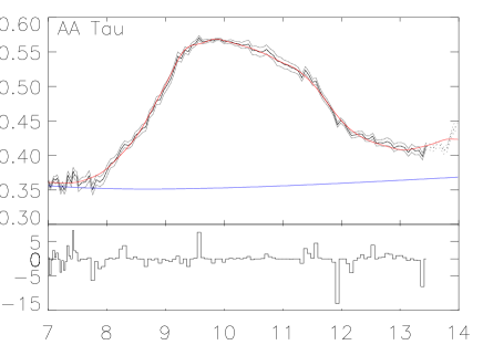
Figure 4: IRS spectrum (black line) and fit (red line) including the corresponding uncertainties (gray lines) of AA Tau as an example of the full data sample. The continuum background used for the fit function is shown in blue. In the lower part of the figure, the resulting $\Delta\chi^{2}$, multiplied by the sign of the deviation, is shown.

Table 3: Derived quantities for the decomposition analysis of the 10 $\mu$m silicate feature. The values in brackets correspond to the border values of the 1$\sigma$ range. The last two columns list the values of the crystallinity for the cold ($\Gamma_{\mathrm{c}}$) and warm ($\Gamma_{\mathrm{w}}$) components as derived by Sargent et al. (2009).

Name	$\Gamma$ [%]		$\chi^{2}_{\mathrm{red}}$	$\Gamma_{\mathrm{c}}$[%]		$\Gamma_{\mathrm{w}}$[0.0pt][%]
04187+1927	$33.4$	($32.6,33.6$)	$2.7$
04303+2240	$33.6$	($32.8,34.4$)	$14.3$
04385+2550	$1.7$	($1.5,1.9$)	$1.8$
AA Tau	$15.6$	($14.4,16.9$)	$1.3$	25$\pm$	21	5$\pm$	5
BP Tau	$8.8$	($8.1,9.1$)	$0.7$	15$\pm$	5	18$\pm$	6
CI Tau	$15.3$	($14.4,16.3$)	$1.7$	8$\pm$	13	6$\pm$	4
CoKu Tau/3	$22.7$	($21.4,24.2$)	$1.8$	18$\pm$	7	11$\pm$	4
CW Tau	$20.7$	($20.1,26.4$)	$2.3$	75$\pm$	27	6$\pm$	9
CY Tau	$37.0$	($32.7,43.1$)	$1.0$	77$\pm$	52	30$\pm$	27
CZ Tau	$2.2$	($2.2,2.3$)	$0.8$
DD Tau	$17.6$	($16.6,18.7$)	$2.2$	19$\pm$	13	20$\pm$	10
DK Tau	$17.3$	($16.7,17.6$)	$2.2$	56$\pm$	14	14$\pm$	3
DN Tau	$44.3$	($41.2,47.2$)	$1.1$	7$\pm$	17	50$\pm$	27
FM Tau	$1.2$	($1.0,1.3$)	$1.2$	13$\pm$	9	4$\pm$	5
FO Tau	$24.7$	($19.1,34.5$)	$0.4$	14$\pm$	7	17$\pm$	11
FQ Tau	$50.7$	($50.1,52.3$)	$1.1$	53$\pm$	153	14$\pm$	8
FS Tau	$1.1$	($1.0,1.2$)	$1.3$	9$\pm$	10	7$\pm$	8
FV Tau	$1.5$	($1.1,2.0$)	$4.9$	6$\pm$	7	8$\pm$	5
FX Tau	$4.6$	($3.9,5.4$)	$1.9$	15$\pm$	6	14$\pm$	4
FZ Tau	$43.1$	($42.1,44.1$)	$2.7$	49$\pm$	28	22$\pm$	7
GH Tau	$34.9$	($31.8,39.0$)	$1.4$	19$\pm$	11	12$\pm$	8
GI Tau	$10.3$	($10.0,11.4$)	$0.5$	13$\pm$	7	3$\pm$	4
GK Tau	$7.7$	($7.6,7.8$)	$1.9$	26$\pm$	9	8$\pm$	3
GN Tau	$17.2$	($16.4,18.9$)	$2.2$	64$\pm$	19	12$\pm$	4
GO Tau	$16.1$	($13.5,19.6$)	$1.1$	14$\pm$	12	9$\pm$	6
Haro 6-13	$1.4$	($1.4,1.5$)	$3.8$
Haro 6-28	$30.3$	($30.1,31.3$)	$1.0$	18$\pm$	11	45$\pm$	13
HK Tau	$40.8$	($37.3,44.5$)	$1.6$	8$\pm$	7	24$\pm$	8
HO Tau	$5.0$	($4.4,5.5$)	$1.2$	17$\pm$	23	14$\pm$	7
HP Tau	$4.1$	($4.0,4.4$)	$1.6$	12$\pm$	24	4$\pm$	4
IQ Tau	$6.9$	($6.4,7.3$)	$1.5$	7$\pm$	31	9$\pm$	5
IS Tau	$29.0$	($26.6,31.7$)	$1.7$	100$\pm$	45	14$\pm$	4
IT Tau	$32.3$	($28.3,40.1$)	$1.7$	8$\pm$	11	63$\pm$	45
MHO-3	$1.5$	($1.4,1.6$)	$13.6$
RY Tau	$7.0$	($6.7,7.5$)	$6.6$
UZ Tau/e	$11.6$	($9.4,11.6$)	$1.1$	5$\pm$	10	2$\pm$	4
V410 Anon 13	$59.1$	($54.6,61.2$)	$1.6$	6$\pm$	7	43$\pm$	13
V710 Tau	$16.2$	($15.3,19.0$)	$1.4$	37$\pm$	21	23$\pm$	10
V773 Tau	$22.4$	($22.4,26.0$)	$2.7$
V807 Tau	$32.1$	($28.6,37.1$)	$1.7$	15$\pm$	7	8$\pm$	18
V955 Tau	$36.5$	($33.8,38.7$)	$1.9$	21$\pm$	9	25$\pm$	8
XZ Tau	$23.5$	($22.0,25.4$)	$1.8$	4$\pm$	14	8$\pm$	12

5 Discussion

5.1 Disk model validity

The fit method presented here for decomposing the 10 $\mu$m silicate feature takes advantage of a continuous temperature distribution. Therefore, this model is more realistic than previous methods using polynomials (Bouwman et al. 2001), single temperature blackbody functions (Meeus et al. 2003) or two temperature fits (e.g. van Boekel et al. 2005 or Sargent et al. 2009). For a systematic comparison between the methods, see Juhasz et al. (2009).

We conclude from the spectral fits that the continuous temperature distribution of the disk is a robust model for approximating the continuum emission. We are able to adjust the background by just one geometrical parameter, i.e. the slope $q$ of the radial temperature distribution, which shows the strength and the simplicity of this method. Although previous studies pointed out that the exact shape of the background function has little effect on the relative composition of the dust mineralogy, the application of a more physical model is appropriate and avoids wrong conclusions about dust temperatures from a single blackbody approach. Further, using the TLTD method to describe the silicate emission features of the disk atmosphere allows to model the contribution to the 10 $\mu$m flux by grains of varying temperatures. As Juhasz et al. (2009) pointed out, this is crucial to reduce the systematic uncertainty of the decomposition.

On the other hand, it has to be mentioned that the temperature profile is assumed to be independent of the dust grain size and composition, which is an evident simplification, especially at the disk surface. Further, the TLTD method in its presented form does not account for radially dependent distributions of the individual dust species. As suggested by Juhasz et al. (2009), to optimize the validity of the applied method, we confined the wavelength range to the 10 $\mu$m feature only and did not include longer wavelengths. It would be very interesting to extend the wavelength range to the full Spitzer IRS spectral coverage; a radially dependent distribution of the dust composition will be implemented in the TLTD method in a future study.

Most objects of our sample have been studied likewise by Sargent et al. (2009) (SA09), using a two temperature decomposition fit (2T fit). Although this method appears to be less realistic, it probes different regions of the disk and is worth to compare with our results. The last two columns of Table 3 list the accumulated values for all crystalline mass fractions for the warm and the cold fit components, respectively. The errors have been calculated using standard error propagation of the uncertainties given in Table 6 of SA09. The method used by SA09 to derive the uncertainties of the fitting parameters is dissimilar from our work and the values for the uncertainties as presented by SA09 are very conservative. The consequence is that large errors appear in the propagated values for the crystallinity as shown in Table 3. Therefore, we expect many objects to have overlaps between the 1 sigma range of our $\Gamma$-values and the values derived by SA09. Indeed, out of 34 common objects, 23 show an overlap with either the warm or the cold component. This number increases to 28 objects when considering our results with a 2 sigma uncertainty. However, such an ad hoc comparison is not very valuable as a real comparison of the derived crystallinity is not possible: Basically, we should compare our results with the warm dust component of SA09 only as this corresponds more likely to the 10 $\mu$m feature. However, the largest fraction of the mass contribution for the two temperature fit is contained in the cold component ($\sim$100 - 200 K) which does not contribute to the 10 $\mu$m flux significantly.

5.2 Correlations between crystallinity and X-ray emission

We compare stellar high-energy properties with structural characteristics of the dust disk. For this purpose, we correlate the X-ray luminosity $L_{\mathrm{X}}$ and the product of $L_{\mathrm{X}}$ and Hardness $H$ with the total crystalline mass fraction $\Gamma$. Using the full sample of the remaining 37 objects shows that these quantities do not correlate. As discussed in Sect. 2, our sample consists of objects of a wide spread in age and therefore it is likely that different evolutionary stages are present even if we are studying class II objects only. As mentioned in Sect. 2, to increase the uniformity of the evolutionary epoch, we selected the objects according their age and divided them into three groups; very young, intermediate and older objects. Unfortunately, our sample size decreases to 34 as we lose another three objects (IRAS 04187+1927, IRAS 04385+2550 and V410 Anon 13) for which no age determination could be found in the literature.

We found a significant correlation between $L_{\mathrm{X}}$ and $\Gamma$ when selecting the objects in the intermediate range ($\sim$1 Myr to $\sim$5 Myr). Figure 5 shows the correlation plots for the three groups while the age limits of 1.1 Myr and 4.5 Myr have been set to optimize the correlation performance with the number of objects used for the intermediate group (see below). We measure a correlation coefficient of -0.62 and a significance of 99.7% for a correlation.

Figure 5: X-ray luminosity $L_{\mathrm{X}}$ vs. total crystalline mass fraction $\Gamma$ for objects of an age within $1.1-4.5$ Myr (top panel), for objects younger than 1.1 Myr (bottom left panel), and older than 4.5 Myr (bottom right panel). The lines in the top panel represent the OLS bisector regression (solid) with the uncertainties for the slope (dashed).

We calculate the regression lines $L_{\mathrm{X}}(\Gamma)$ according the ordinary least square (OLS) bisector method described by Isobe et al. (1990) to treat the two variables symmetrically while we use the logarithmic value of $L_{\mathrm{X}}$ . The dashed lines in Fig. 5 correspond to lines with slopes adding and subtracting the regression slope uncertainty as calculated according to Table 1 of Isobe et al. (1990).

We note here that measurement errors (or errors derived from measurements) will not be used in the derivation of regression lines. If measurement errors are a minor contribution to the scatter around a regression line, then the deviation of a point from the best-fit line is dominated by systematic processes not considered here; using measurement errors as weights for such points will introduce arbitrary bias that is unrelated to the actual scatter of the points. This problem has been discussed in detail by Isobe et al. (1990) and Feigelson & Babu (1992). Is the scatter dominated by unknown, additional processes in our case? The uncertainties in $L_{\rm X}$ of our sample were discussed in Güdel et al. (2007) with the result that the errors resulting from the X-ray measurement process and the spectral fit procedures are usually smaller than variations due to intrinsic X-ray variability on time scales of hours to days. The uncertainty introduced by X-ray variability usually corresponds to a factor of $\sim$2 between maximum and minimum values. As can be seen in our correlation plots discussed here, such variations are smaller than the scatter around the regression lines. We conclude that other factors not considered here dominate the scatter, and errors from the measurement or spectral fit procedures are inappropriate to use here. We therefore use unweighted regression (Isobe et al. 1990).

To define the limits of the stellar age for which the correlation works best, we varied the lower and upper limit and calculated the correlation coefficient of the intermediate group. Figure 6 shows a map of the correlation coefficient and the correlation significance as a function of the minimum and maximum stellar age used for selecting the sample. We see that the minimum and maximum stellar ages for which the correlation is still present, is not sharply defined: It varies between 1-2 Myr for the minimum and 2-4.5 Myr for the maximum age, respectively. This is in agreement with the age uncertainties discussed in Sect. 2. Beside the goodness of the fit, we also considered the statistics in terms of the number of selected objects which is shown in the upper right panel of Fig. 6. Since we tried to optimize the selection in terms of correlation and statistical sample, we show in the lower right panel of the same figure the product of the correlation coefficient and the number of objects. We decided to use objects of age older than 1.1 Myr and younger than 4.5 Myr and 20 objects satisfied this condition while 14 objects fall outside the borders. We emphasize that these age limits are somewhat arbitrary within the typical age uncertainties adopted for our stellar ages (see Sect. 2) and correspond to an optimum choice based on the limited number of objects in our sample. The selected age interval should be interpreted as essentially containing CTTS of typical ages in Taurus ($\approx 1-5$ Myr). We marked the final selection with a circle in Fig. 6.

Since we selected the sample according the goodness of decompositional fit of the 10 $\mu$m feature using $\chi^{2}_{\mathrm{red}}\leq 3$ as a criterium, we investigated how this cut effects the correlation. For this purpose we added all objects to the sample within the optimum age limits but higher $\chi^{2}_{\mathrm{red}}$, in particular we added MHO-3 and RY Tau. The correlation coefficient of this enlarged sample was found to be -0.63 with a probability of 99.6%. This is very comparable to the original result and we conclude that the applied threshold for $\chi^{2}_{\mathrm{red}}$ has no influence on the systematics of our study.

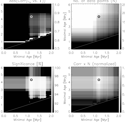
Figure 6: Maps of the correlation coefficient (absolute value, upper left), the number of selected data points (upper right), the significance (lower left) and the product of the correlation coefficient and the number of selected datapoint (lower right) for the $L_{\mathrm{X}}$ vs. $\Gamma$ correlation taking only objects into consideration which have a stellar age in between the minimum and the maximum age as indicated by the two axes of the maps. The circles indicate our selection of the stellar age for which the correlation coefficient and the statistics has been optimized. The straight lines indicate where the minimum and maximum age limitations are identical.

Finally, we plot in Fig. 7 the product of $L_{\mathrm{X}}$ and $H$ against $\Gamma$, using the same object selection as before.

Figure 7: Product of the X-ray luminosity $L_{\mathrm{X}}$ and the X-ray hardness $H$ vs. total crystalline mass fraction $\Gamma$ for objects of an age within $1.1-4.5$ Myr (top panel), for objects younger than 1.1 Myr (bottom left panel), and older than 4.5 Myr (bottom right panel).

We measure a correlation coefficient of -0.66 with a significance of 99.9%. The product of $L_{\mathrm{X}}$ and $H$ may represent the deposited energy of the X-rays in the disk. It is remarkable that the correlation for the product of $L_{\mathrm{X}}$ and the hardness correlate better with the crystalline mass fraction than the X-ray luminosity alone. We investigated the optimum age selection limits as before, and got for both the minimum and maximum age identical values as derived for the $L_{\mathrm{X}}$ vs. $\Gamma$ correlation.

We repeated this study with the values of the crystalline mass fraction derived by SA09 to discuss the dependencies of the correlation on the applied method. Therefore, we correlated the crystalline mass fractions $\Gamma_{\mathrm{c}}$ and $\Gamma_{\mathrm{w}}$ (see Sect. 5.1 and Table 3) with $L_{\mathrm{X}}$ . Since the reduced $\chi^{2}_{\mathrm{red}}$ in SA09 are systematically high, we had to increase the limit to $\chi^{2}_{\mathrm{red}}\leq 5$ to calculate the correlation with a sufficient sample. With this approach we use a sample of 20 common objects of which 14 fall into the age range of 1.1-4.5 Myr. We found that $\Gamma_{\mathrm{w}}$ correlates weakly with $L_{\mathrm{X}}$ (corr=-0.54, $P$=95.6 %) and strongly with $H\cdot L_{\mathrm{X}}$ (corr=-0.65, $P$=98.9 %). $\Gamma_{\mathrm{c}}$ does not correlate with any of these parameters at all. Further, repeating the investigation of the age range selection showed a comparable picture to the valid range (1.1-1.5 Myr for the lower limit and 1.5-6 Myr for the upper limit).

This result confirms three aspects of our study: First, the correlation seems to be independent of the applied fitting method and is therefore not biased by the systematics of the decomposition approach. Second, our TLTD fit refers to the 10 $\mu$m feature, for which we found a correlation between crystallinity and $L_{\mathrm{X}}$ . In the 2T fit (as used by SA09), the 10 $\mu$m feature is emitted by the warm component, and a corresponding correlation is indeed found. Our focus on the 10 $\mu$m silicate feature is therefore justified a posteriori as the cold component from the 2T fit does not show a correlation. And third, we see in both data sets that the correlation for the combined product of hardness and X-ray luminosity is better than for the X-ray luminosity alone.

5.3 Is the dust amorphized by the stellar wind?

It is a remarkable result that an anticorrelation between the X-ray emission and the crystalline mass fraction is found; so far, no correlation between properties of the central object and the crystalline structure of the dust disk has been reported from observations (e.g., Sicilia-Aguilar et al. 2007).

However, the observed anticorrelation demands an indirect explanation because X-rays of the observed energies carry too little momentum to damage the crystalline structure of the dust. Their energy will rather be absorbed by the electrons, which temporarily leads to ionization of lattice atoms and finally to the production of phonons and a resulting increase of the temperature within the grain.

Although the processes of X-ray emission are still controversial for T Tauri objects, it seems clear that they mostly originate in magnetic coronae analogous to the solar corona, although stellar coronae are much more X-ray luminous and hotter. Therefore, we assume that the X-ray emission of our sample of T Tauri stars is related to the high energy processes in the stellar corona that also lead to a solar-like wind composed of ions, electrons and neutrons. We show in the following that the flux of the solar wind and the particle energies would be sufficient to amorphize dust grains efficiently in a protoplanetary disk at a radius of 1 AU and that this process induces significant changes in the emission profile of the dust grains. Although we may observe the silicates at larger distances from their central object, the choice of 1 AU is based on the availability of data from the solar wind and allows for an extrapolation to larger distances. We use a simple disk model where homogeneous dust grains at the disk surface are directly exposed to the stellar wind and where recrystallization effects are neglected.

5.3.1 Stellar wind properties

We first derive the particle fluxes and energies from data from the solar wind as this is the only object for which direct and reliable measurements of these parameters are available. We know from the enrichment of spallation products in meteorites that the young Sun had a proton flux several orders of magnitude higher than at present (Caffe et al. 1987). Unfortunately, the energies which lead to nuclear spallation are in the order of $E>10\leavevmode\nobreak\$MeV while the energies of interest for amorphization are $E<1\leavevmode\nobreak\$MeV (see below and, e.g., Jäger et al. 2003). The processes producing these energies might be different and consequently it may not be correct to scale particle fluxes with the well measured soft X-ray flux for younger stars. Therefore, we proceed with present solar particle fluxes and energies and use its amorphization potential as a lower limit.

We used the database from OMNIWeb (King & Papitashvili 2005) to determine the present proton density of the solar wind plasma, its velocities and proton to He-ion ratio near the Earth. We averaged the full dataset over the years 1963 until 2008 and obtained a density of $\sim$7.2 protons/cm³, a wind speed of $\sim$450 km/s and a He-ion to proton ratio of $\sim$4.4 %. Uncertainties of these quantities are up to 30 %. This leads to a mean proton flux of 3.2$\cdot 10^{8}$ protons/(cm${}^{2}\cdot$s) at energies around 1 keV and to a He-ion flux of 1.4$\cdot 10^{7}$ ions/(cm${}^{2}\cdot$s) at energies around 4 keV.

5.3.2 Calculation of dust amorphization

We use these values to compare them with the ion dose required to amorphize a dust grain. For this purpose we calculate the number of displacements of lattice atoms per incident ion using the SRIM-2008 software (Ziegler et al. 2008). SRIM is a collection of software packages which calculate many features of the transport of ions in matter such as ion stopping, range and straggling distributions in multilayer targets of any material. Further, it allows the calculation of ion implantation including damages to solid targets by atom displacement, sputtering and transmission in mixed gas/solid targets. Table 4 summarizes the calculation performed for two minerals, pyroxene and enstatite, respectively, irradiated by protons and He-ions at various energies. With the SRIM software we determined the penetration depth (range) of the ion and the number of displaced lattice atoms (due to elastic scattering on the atom’s nuclei) per incident ion.

Table 4: Ion-penetration depth (range), number of displaced lattice atoms per ion $N_{\mathrm{Disp.}}/\mathrm{ion}$, and the minimum required dose for full amorphization of the upper layer (of thickness equal to the ion penetration depth) of pyroxene and enstatite by proton and He-ion irradiation at various energies. For this calculation, mineral data from the webmineral data base and the calculation software SRIM-2008 (Ziegler et al. 2008) have been used. For the calculation of the dose, a minimal displacement per lattice atom (dpa) of 2.5 have been assumed to observe amorphization.

Ion	Stellar Wind	Particle	Pyroxene, $\rho=1.2\cdot 10^{23}\frac{\mathrm{atoms}}{\mathrm{cm}^{3}}$			Enstatite, $\rho=9.6\cdot 10^{22}\frac{\mathrm{atoms}}{\mathrm{cm}^{3}}$
	Speed	Energy	Range	$\frac{N_{\mathrm{Disp.}}}{\textrm{ion}}$	Dose	Range	$\frac{N_{\mathrm{Disp.}}}{\textrm{ion}}$	Dose
	[km/s]	[keV]	[nm]		$\cdot 10^{16}\leavevmode\nobreak\ \frac{\mathrm{ions}}{\mathrm{cm}^{2}}$	[nm]		$\cdot 10^{16}\leavevmode\nobreak\ \frac{\mathrm{ions}}{\mathrm{cm}^{2}}$
p+	$300$	$0.5$	$8.3$	$0.8$	$30.7$	$9.4$	$0.8$	$28.2$
	$400$	$0.8$	$12$	$1.5$	$23.7$	$10.7$	$1.5$	$17.1$
	$450$	$1.1$	$15.8$	$2.1$	$22.3$	$17.3$	$2.1$	$19.8$
	$500$	$1.3$	$17.7$	$2.4$	$21.8$	$19.6$	$2.5$	$18.8$
	$600$	$1.9$	$24.4$	$3.3$	$21.9$	$26.6$	$3.3$	$19.3$
	$700$	$2.6$	$31.7$	$4$	$23.5$	$35.5$	$4.1$	$20.8$
	$800$	$3.3$	$38.8$	$4.7$	$24.4$	$43$	$4.8$	$21.5$
	$1384$	$10.0$	$97.2$	$8.2$	$35.1$	$107.1$	$8.1$	$31.7$
	$3094$	$50.0$	$332.7$	$12.6$	$78.2$	$364.5$	$12.4$	$70.6$
He	$300$	$1.9$	$14.4$	$20.1$	$2.1$	$15.5$	$19.4$	$1.9$
	$400$	$3.3$	$23.4$	$31.1$	$2.2$	$26.3$	$31.1$	$2.0$
	$450$	$4.2$	$29.1$	$36.9$	$2.3$	$33.6$	$36.6$	$2.2$
	$500$	$5.2$	$35.7$	$42.6$	$2.5$	$40.1$	$42.3$	$2.3$
	$600$	$7.5$	$50.5$	$53.3$	$2.8$	$56.5$	$52.8$	$2.6$
	$700$	$10.2$	$67.5$	$63.8$	$3.1$	$74.3$	$62.7$	$2.8$
	$800$	$13.3$	$84.9$	$72.7$	$3.5$	$95.5$	$71$	$3.2$
	$1553$	$50.0$	$263.4$	$116.2$	$6.7$	$292$	$113$	$6.2$

The mineral densities have been taken from the webmineral database. We determine the required ion dose for complete amorphization of the dust grain material down to the penetration depth of the incident ion by deriving the column density of the lattice atoms. Further, we require a quantity for how many displacements per lattice atom (dpa) are required to observe amorphization. We set this number to be 2.5 based on the mineral irradiation experiments for enstatite (Jäger et al. 2003), forsterite (Bringa et al. 2007) and olivine (Demyk et al. 2001; Carrez et al. 2002). However, this quantity remains inaccurate as most of the above cited studies determined doses for He-irradiation to fully amorphize the minerals varying within an order of magnitude. Jäger et al. (2003) presented a dpa-value of 2.5 but the lowest He-ion energy used was 50 keV. For protons, we assume the same dpa ratio although this is hypothetical.

Table 4 further shows that $N_{\mathrm{Disp}}/\mathrm{ion}$ increases with increasing energy but the required dose for amorphization increases as well. This can be explained from the definition of the required dose. With higher energies, the ions penetrate deeper into the dust grain and consequently a thicker layer will be amorphized. This requires a larger total number of displacements as more lattice atoms are impacted.

We can therefore conclude from this calculation that the He-ions of the present solar wind would amorphize the top $\sim$30 nm of the irradiated face of a pyroxene dust grain and the required dose of $\sim$2.3$\cdot 10^{16}\leavevmode\nobreak\ \mathrm{ions}/\mathrm{cm}^{2}$ would be accumulated within $\sim$50 years. To allow the full surface to be amorphized, the dust grain has to rotate with respect to the ion beam to allow for an isotropic irradiation, and the timescale has to be increased by a factor of a few. Obviously this indicates a very efficient mechanism for amorphization and might be even more efficient as we have ignored the irradiation by other ions.

On the other hand, this calculation assumes that all dust grains are fully exposed to the radiation of the central object. This is obviously not true for the majority of the observable grains in the disk atmosphere. The ion flux gets extinct analogue to optical light due to absorption by dust grains (self-shielding) and therefore, the amorphization timescale depends strongly on the location of the grain within the disk and the presence of vertical mixing of the disk material. Therefore, the 50 years of irradiation time represent the timescale for amorphization, based on the full flux. This number will increase exponentially (or faster) the deeper the grains are located in the disk. Consequently, our observations probe various timescales for dust amorphization; conclusions depending on whether the presented mechanisms are too efficient or too inefficient cannot be made at the present time. Knowing the mean free path length along the particle trajectories would enable more quantitative conclusions about the amorphization timescale and potential with respect to other dust processing mechanisms. Particles of higher energies could also be considered by studying multiple scattering of ions with dust grains. This would allow an amorphization of dust deeper in the disk. For this purpose, dedicated modeling of the disk geometry and grain size distribution is required. This will be addressed in future studies.

For now, we can conclude that the dust amorphization by stellar wind ions at the disk surface is sufficiently efficient so that this mechanism might dominate the dust processing at the disk surface layer.

5.3.3 Optical properties and grain size dependency

Since the dust grains are amorphized only at the surface layer, the impact on the optical emissivity has to be investigated to demonstrate the observability of the amorphization of circumstellar dust by the low energetic stellar wind.

As an example, we calculate the optical mass absorption coefficients of crystalline pyroxene, coated with a 30 nm thick layer of amorphous pyroxene using Mie theory according to Bohren & Huffman (1983) for coated spheres. The calculation code in the appendix B of Bohren & Huffman (1983) has been translated by Mätzler (2002) into a Matlab script which we have used for this study. The optical constants from Jäger et al. (1994) were used for crystalline pyroxene while parameters for the amorphous pyroxene are taken from Dorschner et al. (1995).

Figure 8 shows the resulting mass absorption coefficient within the wavelength range of interest for a dust grain of 0.1 $\mu$m and 1.26$\mu$m in radius, respectively.

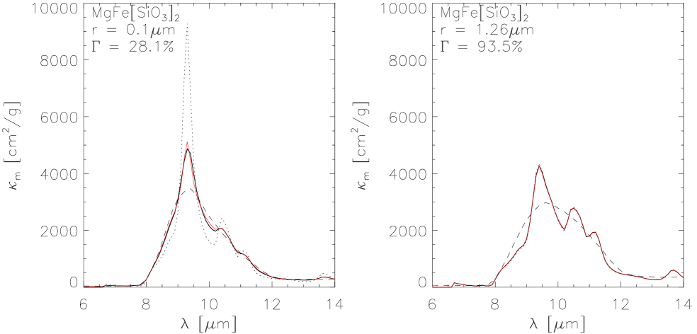
Figure 8: The thick, solid line corresponds to the mass absorption coefficient of a 2-layer spherical dust grain with pyroxene stoichiometry and a radius of 0.1 $\mu$m (left) and 1.26 $\mu$m (right). The outer layer is amorphous with a thickness of 30 nm in both cases and the core is crystalline. The dotted line corresponds to a pure crystalline and the dashed line to a pure amorphous grain of the same size and chemical composition. The red, thin solid line shows a decomposition fit of the 2-layer absorption coefficient with a purely amorphous and purely crystalline component and a crystalline mass fraction of $\Gamma$=28.1% and $\Gamma$=93.5% is measured, respectively. Due to the high crystalline mass fraction for the larger grain, the dotted, red and thick lines overlap in the right panel.

Further, this plot indicates the two extremes of a purely crystalline grain and a purely amorphous pyroxene grain. Finally, we calculate a linear combination of the two extremes to fit the 2-layer case and get a contribution ratio for the crystalline dust of $\Gamma$=28.1% for the 0.1 $\mu$m grain and $\Gamma$=93.5% for the 1.26 $\mu$m grain, where $\Gamma$ corresponds to the same definition as used for the decomposition fits. This result reflects the mass ratio used for the coated sphere calculation (29.1% crystalline for the 0.1 $\mu$m grain and 93.0% for the 1.26 $\mu$m grain) with relatively high accuracy. Consequently, even if the dust grains are amorphized in the surface layer only, the spectrally derived value for amorphization corresponds to the mass ratio of crystalline and amorphous silicates and conclusions about dust amorphization are valid even for low-energy ions.

However, the provided calculation assumes a purely crystalline dust grain. We expect to see a mixture of amorphous and crystalline dust regardless of the stellar wind and its impact on the dust structure. Consequently, the model described here delivers only an additional component for the amorphous dust content and values for $\Gamma$ are expected to be lower than these limits.

Further, the results of the decompositional fits of our sample (see Table A) suggest that a significant amount of the dust is present in larger grains and hence, the discussed mechanism might not be applicable. However, we repeated this study considering only small grains and no correlation between $L_{\mathrm{X}}$ and $\Gamma$ was found. It is very likely that higher energetic ions are important and more abundant than in the present solar system. These ions penetrate deeper into the dust grain and consequently, larger grains are amorphized. Therefore, the approach of using a monochromatic ion beam with solar wind properties is too elementary and has to be extended for more quantitative studies.

6 Conclusions

The previous calculations show that the amorphization of the surface layer of the protoplanetary dust by the stellar wind is a viable scenario. We have seen that a stellar wind with solar characteristics allows a very fast amorphization of the upper layer of dust grains compared to the longer timescales of dust processing during the star and disk formation. For sub-micron grains, this process leads to an observable structural change of the grain.

However, these processes are inefficient for micron-sized grains or larger bodies as the penetration depth of the low-energetic ions are too small to degrade the dust sufficiently.

On the other hand, as young stars are generally more active, we can assume that particle fluxes and energies are generally higher than in the present solar wind and consequently, the described processes may be even more efficient. Further, the solar irradiation is not only composed of the solar wind but a great variety of additional particles at various energies and fluxes. Since our knowledge of these particle fluxes ($E\la$10 MeV) in the early time of the solar history is very poor, and since particle irradiation in other systems are unmeasurable, the assessment of the amorphization efficiency remains very inaccurate and difficult. Other irradiation sources than the star, such as shocks from stellar winds in the protoplanetary gas disk or from accretion or jets confuse the overall picture further. Recrystallization due to thermal annealing of warmer dust grains (see, e.g., Djouadi et al. 2005) may inhibit the amorphization process and needs to be taken into account for quantitative models.

Nonetheless, we observe a correlation for 20 objects between the X-ray luminosity as well as the X-ray luminosity multiplied with the X-ray hardness and the crystalline mass fraction of the atmospheric dust of the inner protoplanetary disk for objects within an age range of approx. 1 to 4.5 Myr. We interpret this as an indicator of high-energy processes in the central object. We therefore postulate degenerative processes for the crystalline structure of the dust by ionic irradiation. Although we cannot observe the stellar wind directly, its flux and/or speed might be related to the X-ray luminosity, as shown for low X-ray fluxes by Wood et al. (2005) by comparing stellar mass loss rates with X-ray surface fluxes.

Self-shielding effects of the dust disk play an important role for the time scale and the overall potential of amorphization. Consequently, the disk geometry and the dust density distribution have to be taken into account for studying evolutionary effects. Further, self-shielding could explain why the correlation diminishes if we include objects younger than $\sim$1 Myr. These objects might have well mixed disks even in the upper disk atmosphere where dust settling has poorly progressed; consequently, the self-shielding is more relevant.

It is less clear why the correlation worsens if we include objects older than $\sim$4.5 Myr. It could be related to a statistical problem as our sample does not include many objects at such ages. Further physical effects may also play a role on longer time scales. Possibilities include radial dust mixing or the reproduction of crystalline dust material in the inner disk region.

It would be interesting to verify if this correlation is present in other star forming regions and for a larger sample of objects. The extension of this study to Herbig Ae/Be systems could provide different aspects of this process due to the shorter evolutionary time scales of the central object.

Appendix A Resulting fit parameters

Table 5: Resulting fit parameters for the decomposition analysis of the 10 $\mu$m silicate feature. Dashes indicate that the lower boundary has been reached and the component proportion has been set to 0.

Name	$q_{\mathrm{disk}}$	MgFeSiO4		MgFe[SiO3]2		Mg2SiO4		MgSiO3		SiO2
	$\times 10^{-1}$	Small [%]	Large [%]	Small [%]	Large [%]	Small [%]	Large [%]	Small [%]	Large [%]	Small [%]	Large [%]
04187+1927	$-6.32_{-0.01}^{+0.01}$	$-$	$-$	$12.8_{-2.0}^{+0.1}$	$53.7_{-0.1}^{+3.1}$	$-$	$10.4_{-0.5}^{+0.1}$	$1.9_{-0.3}^{+0.0}$	$15.7_{-0.1}^{+0.1}$	$4.8_{-0.0}^{+0.1}$	$0.7_{-0.0}^{+0.1}$
04303+2240	$-5.84_{-0.08}^{+0.09}$	$-$	$66.4_{-0.8}^{+0.8}$	$-$	$-$	$7.1_{-0.2}^{+0.2}$	$18.2_{-0.6}^{+0.6}$	$-$	$-$	$-$	$8.4_{-0.0}^{+0.0}$
04385+2550	$-4.35_{-0.08}^{+0.07}$	$32.4_{-0.2}^{+0.2}$	$47.6_{-3.6}^{+4.6}$	$-$	$18.3_{-4.0}^{+3.7}$	$0.0_{-0.0}^{+0.0}$	$1.7_{-0.1}^{+0.2}$	$-$	$-$	$-$	$-$
AA Tau	$-6.07_{-0.21}^{+0.16}$	$29.0_{-1.4}^{+1.5}$	$-$	$-$	$55.4_{-3.3}^{+2.6}$	$0.0_{-0.0}^{+0.0}$	$5.9_{-0.7}^{+0.7}$	$-$	$7.3_{-0.6}^{+0.8}$	$-$	$2.4_{-0.1}^{+0.1}$
BP Tau	$-5.50_{-0.36}^{+0.19}$	$44.5_{-2.1}^{+1.2}$	$0.0_{-0.0}^{+5.3}$	$9.9_{-0.9}^{+1.6}$	$37.0_{-6.6}^{+1.1}$	$1.2_{-0.0}^{+0.0}$	$4.4_{-0.3}^{+0.2}$	$2.6_{-0.4}^{+0.5}$	$-$	$-$	$0.6_{-0.5}^{+0.2}$
CI Tau	$-5.29_{-0.11}^{+0.11}$	$21.0_{-0.6}^{+0.7}$	$-$	$-$	$63.7_{-1.7}^{+1.7}$	$2.1_{-0.1}^{+0.1}$	$6.1_{-0.5}^{+0.5}$	$-$	$3.4_{-0.4}^{+0.4}$	$-$	$3.8_{-0.0}^{+0.0}$
CoKu Tau/3	$-5.51_{-0.17}^{+0.15}$	$-$	$-$	$-$	$77.3_{-1.4}^{+1.3}$	$3.4_{-0.1}^{+0.1}$	$9.6_{-0.7}^{+0.8}$	$-$	$6.7_{-0.7}^{+0.8}$	$-$	$3.0_{-0.2}^{+0.2}$
CW Tau	$-7.50_{-0.14}^{+0.05}$	$0.0_{-0.0}^{+21.7}$	$-$	$-$	$79.3_{-27.5}^{+0.6}$	$3.8_{-0.0}^{+0.2}$	$4.8_{-0.3}^{+2.6}$	$-$	$7.3_{-0.3}^{+3.7}$	$-$	$4.8_{-0.8}^{+0.0}$
CY Tau	$-5.43_{-0.60}^{+0.49}$	$-$	$-$	$40.9_{-0.3}^{+1.9}$	$22.3_{-8.2}^{+4.6}$	$3.4_{-0.0}^{+0.1}$	$14.0_{-1.4}^{+2.2}$	$0.0_{-0.0}^{+0.5}$	$11.0_{-2.8}^{+3.3}$	$0.4_{-0.3}^{+0.2}$	$8.2_{-0.2}^{+0.2}$
CZ Tau	$-5.10_{-0.02}^{+0.01}$	$15.3_{-0.6}^{+1.0}$	$-$	$41.7_{-1.0}^{+0.6}$	$40.8_{-0.0}^{+0.1}$	$0.8_{-0.1}^{+0.0}$	$-$	$1.4_{-0.1}^{+0.1}$	$-$	$-$	$0.0_{-0.0}^{+0.0}$
DD Tau	$-5.59_{-0.29}^{+0.20}$	$0.0_{-0.0}^{+7.6}$	$0.0_{-0.0}^{+24.4}$	$4.9_{-2.3}^{+8.6}$	$71.2_{-25.4}^{+7.1}$	$1.5_{-0.0}^{+0.1}$	$5.5_{-0.2}^{+0.8}$	$1.7_{-1.2}^{+0.1}$	$7.2_{-0.2}^{+1.1}$	$-$	$1.9_{-1.3}^{+0.1}$
DK Tau	$-4.78_{-0.08}^{+0.09}$	$-$	$0.0_{-0.0}^{+1.4}$	$1.7_{-0.7}^{+1.4}$	$80.6_{-1.1}^{+0.5}$	$3.5_{-0.1}^{+0.1}$	$3.4_{-0.2}^{+0.1}$	$7.1_{-0.3}^{+0.2}$	$-$	$0.3_{-0.0}^{+0.0}$	$3.0_{-0.1}^{+0.0}$
DN Tau	$-5.74_{-0.14}^{+0.20}$	$-$	$-$	$12.1_{-0.6}^{+0.6}$	$43.8_{-3.1}^{+4.3}$	$3.0_{-0.0}^{+0.0}$	$14.7_{-0.9}^{+0.7}$	$-$	$17.7_{-2.3}^{+2.2}$	$1.1_{-0.0}^{+0.1}$	$7.8_{-0.0}^{+0.0}$
FM Tau	$-4.81_{-0.14}^{+0.17}$	$57.1_{-0.5}^{+0.4}$	$13.1_{-3.6}^{+3.5}$	$-$	$28.8_{-3.8}^{+3.7}$	$0.8_{-0.0}^{+0.0}$	$-$	$0.0_{-0.0}^{+0.3}$	$-$	$-$	$0.2_{-0.2}^{+0.4}$
FO Tau	$-5.65_{-0.76}^{+0.60}$	$-$	$-$	$25.2_{-0.5}^{+4.6}$	$50.3_{-13.5}^{+5.9}$	$2.9_{-0.1}^{+0.1}$	$2.8_{-0.8}^{+1.8}$	$0.0_{-0.0}^{+0.4}$	$17.2_{-5.9}^{+8.3}$	$1.2_{-0.4}^{+0.1}$	$0.7_{-0.7}^{+1.0}$
FQ Tau	$-8.11_{-0.06}^{+0.04}$	$-$	$-$	$-$	$49.3_{-1.6}^{+0.6}$	$-$	$17.7_{-0.4}^{+1.1}$	$2.5_{-0.0}^{+0.1}$	$24.8_{-0.2}^{+0.3}$	$0.1_{-0.1}^{+0.0}$	$5.6_{-0.1}^{+0.3}$
FS Tau	$-5.21_{-0.06}^{+0.08}$	$20.2_{-0.5}^{+0.4}$	$56.4_{-1.8}^{+1.4}$	$-$	$22.3_{-1.9}^{+2.5}$	$1.1_{-0.1}^{+0.1}$	$-$	$0.0_{-0.0}^{+0.1}$	$-$	$-$	$0.0_{-0.0}^{+0.0}$
FV Tau	$-4.31_{-0.06}^{+0.04}$	$-$	$98.5_{-0.5}^{+0.4}$	$-$	$-$	$0.3_{-0.0}^{+0.0}$	$0.5_{-0.4}^{+0.6}$	$-$	$-$	$-$	$0.7_{-0.1}^{+0.1}$
FX Tau	$-4.71_{-0.09}^{+0.08}$	$40.5_{-0.5}^{+0.6}$	$-$	$-$	$54.9_{-1.4}^{+1.2}$	$2.4_{-0.1}^{+0.1}$	$0.6_{-0.4}^{+0.6}$	$1.5_{-0.2}^{+0.3}$	$-$	$-$	$0.2_{-0.1}^{+0.1}$
FZ Tau	$-4.94_{-0.15}^{+0.15}$	$-$	$48.9_{-7.6}^{+6.0}$	$-$	$8.0_{-8.0}^{+8.6}$	$4.2_{-0.0}^{+0.0}$	$11.9_{-0.0}^{+0.1}$	$13.2_{-0.3}^{+0.2}$	$6.8_{-1.0}^{+1.0}$	$5.0_{-0.2}^{+0.2}$	$2.1_{-0.5}^{+0.5}$
GH Tau	$-6.64_{-0.41}^{+0.37}$	$-$	$-$	$0.0_{-0.0}^{+1.1}$	$65.1_{-3.7}^{+2.2}$	$0.1_{-0.1}^{+0.1}$	$12.3_{-1.0}^{+1.5}$	$-$	$20.6_{-2.5}^{+3.1}$	$1.2_{-0.0}^{+0.0}$	$0.8_{-0.3}^{+0.2}$
GI Tau	$-5.73_{-0.19}^{+0.13}$	$45.1_{-1.0}^{+1.3}$	$-$	$0.0_{-0.0}^{+1.1}$	$44.5_{-2.3}^{+0.3}$	$1.4_{-0.0}^{+0.1}$	$2.9_{-0.1}^{+0.6}$	$0.1_{-0.1}^{+0.0}$	$3.9_{-0.2}^{+0.6}$	$-$	$2.1_{-0.2}^{+0.1}$
GK Tau	$-4.61_{-0.10}^{+0.09}$	$43.2_{-0.6}^{+0.7}$	$-$	$15.2_{-1.6}^{+1.4}$	$34.0_{-0.7}^{+0.8}$	$3.2_{-0.0}^{+0.0}$	$0.4_{-0.0}^{+0.0}$	$2.6_{-0.1}^{+0.1}$	$-$	$-$	$1.4_{-0.0}^{+0.0}$
GN Tau	$-5.11_{-0.18}^{+0.10}$	$-$	$-$	$-$	$82.8_{-1.7}^{+0.9}$	$3.5_{-0.1}^{+0.2}$	$3.0_{-0.4}^{+0.8}$	$-$	$5.5_{-0.4}^{+0.8}$	$2.7_{-0.1}^{+0.0}$	$2.5_{-0.0}^{+0.0}$
GO Tau	$-5.40_{-0.28}^{+0.36}$	$-$	$-$	$0.3_{-0.3}^{+4.3}$	$82.1_{-2.3}^{+1.4}$	$0.8_{-0.1}^{+0.1}$	$1.7_{-0.6}^{+1.4}$	$-$	$13.7_{-2.2}^{+1.9}$	$-$	$-$
Haro 6-13	$-3.81_{-0.03}^{+0.03}$	$11.8_{-0.0}^{+0.0}$	$61.7_{-1.6}^{+1.9}$	$-$	$25.0_{-2.0}^{+1.7}$	$1.4_{-0.1}^{+0.1}$	$-$	$-$	$-$	$-$	$-$
Haro 6-28	$-6.97_{-0.06}^{+0.03}$	$-$	$-$	$-$	$69.7_{-1.0}^{+0.2}$	$5.6_{-0.0}^{+0.3}$	$-$	$15.4_{-0.1}^{+0.5}$	$8.0_{-0.1}^{+0.0}$	$0.5_{-0.3}^{+0.0}$	$0.7_{-0.1}^{+0.6}$
HK Tau	$-4.75_{-0.00}^{+0.58}$	$8.3_{-0.0}^{+2.9}$	$34.1_{-34.1}^{+0.0}$	$-$	$16.8_{-0.0}^{+39.3}$	$1.2_{-0.0}^{+1.0}$	$17.2_{-0.0}^{+2.4}$	$13.7_{-0.0}^{+0.2}$	$8.8_{-8.8}^{+0.0}$	$-$	$0.0_{-0.0}^{+1.8}$
HO Tau	$-4.38_{-0.38}^{+0.18}$	$34.9_{-0.7}^{+0.2}$	$0.0_{-0.0}^{+11.1}$	$-$	$59.7_{-9.3}^{+0.7}$	$2.1_{-0.3}^{+0.2}$	$0.9_{-0.4}^{+0.5}$	$-$	$-$	$0.2_{-0.1}^{+0.1}$	$2.0_{-0.7}^{+0.1}$
HP Tau	$-4.82_{-0.08}^{+0.11}$	$47.1_{-0.2}^{+0.4}$	$3.5_{-3.5}^{+2.2}$	$-$	$45.6_{-2.3}^{+3.3}$	$2.5_{-0.0}^{+0.1}$	$-$	$-$	$-$	$-$	$1.7_{-0.1}^{+0.2}$
IQ Tau	$-5.41_{-0.28}^{+0.33}$	$12.0_{-0.7}^{+1.0}$	$60.4_{-7.5}^{+5.8}$	$-$	$20.8_{-5.2}^{+7.0}$	$2.6_{-0.0}^{+0.0}$	$-$	$-$	$1.3_{-0.7}^{+0.6}$	$-$	$2.9_{-0.3}^{+0.3}$
IS Tau	$-4.64_{-0.19}^{+0.18}$	$-$	$-$	$-$	$71.0_{-2.6}^{+2.6}$	$4.8_{-0.3}^{+0.3}$	$8.3_{-1.1}^{+1.2}$	$3.9_{-0.4}^{+0.4}$	$4.4_{-0.5}^{+0.6}$	$2.8_{-0.1}^{+0.1}$	$4.9_{-0.2}^{+0.2}$
IT Tau	$-5.58_{-0.29}^{+0.28}$	$-$	$-$	$-$	$67.7_{-7.4}^{+4.7}$	$-$	$3.1_{-0.5}^{+1.8}$	$1.0_{-1.0}^{+0.3}$	$28.0_{-2.8}^{+6.1}$	$0.0_{-0.0}^{+0.4}$	$-$
MHO-3	$-3.43_{-0.02}^{+0.02}$	$39.9_{-0.0}^{+0.0}$	$37.4_{-1.1}^{+1.1}$	$-$	$21.2_{-1.1}^{+1.2}$	$1.1_{-0.1}^{+0.1}$	$0.4_{-0.0}^{+0.0}$	$-$	$-$	$-$	$-$
RY Tau	$-5.40_{-0.11}^{+0.05}$	$47.5_{-0.4}^{+0.5}$	$-$	$-$	$45.5_{-1.5}^{+0.7}$	$2.2_{-0.1}^{+0.1}$	$2.7_{-0.2}^{+0.3}$	$0.9_{-0.1}^{+0.1}$	$-$	$-$	$1.2_{-0.0}^{+0.0}$
UZ Tau/e	$-6.30_{-1.31}^{+0.16}$	$11.3_{-11.3}^{+0.4}$	$44.4_{-2.1}^{+37.5}$	$0.0_{-0.0}^{+8.1}$	$32.8_{-32.8}^{+2.5}$	$0.9_{-0.1}^{+0.0}$	$2.8_{-2.0}^{+0.1}$	$-$	$4.7_{-0.3}^{+0.9}$	$-$	$3.1_{-1.1}^{+0.1}$
V410 Anon 13	$-6.93_{-0.09}^{+0.35}$	$-$	$-$	$11.8_{-2.7}^{+0.9}$	$30.0_{-3.9}^{+5.6}$	$14.6_{-0.8}^{+0.5}$	$16.4_{-1.3}^{+0.8}$	$23.3_{-2.2}^{+1.4}$	$3.2_{-0.1}^{+0.7}$	$1.2_{-0.2}^{+0.2}$	$-$
V710 Tau	$-3.98_{-1.02}^{+0.17}$	$-$	$0.0_{-0.0}^{+40.5}$	$23.3_{-2.7}^{+3.0}$	$61.1_{-46.9}^{+1.8}$	$0.4_{-0.4}^{+0.1}$	$4.3_{-0.3}^{+0.2}$	$0.0_{-0.0}^{+0.8}$	$6.6_{-1.0}^{+4.2}$	$-$	$4.9_{-2.1}^{+0.2}$
V773 Tau	$-4.56_{-0.22}^{+0.00}$	$-$	$69.8_{-0.0}^{+2.4}$	$-$	$7.9_{-7.9}^{+0.0}$	$5.3_{-0.0}^{+0.7}$	$6.3_{-0.0}^{+0.9}$	$-$	$10.8_{-0.0}^{+2.0}$	$-$	$-$
V807 Tau	$-7.26_{-0.39}^{+0.47}$	$-$	$-$	$-$	$67.9_{-4.6}^{+3.6}$	$5.3_{-0.3}^{+0.4}$	$10.4_{-1.3}^{+1.9}$	$-$	$16.3_{-3.1}^{+2.8}$	$-$	$0.0_{-0.0}^{+1.3}$
V955 Tau	$-5.53_{-0.17}^{+0.20}$	$-$	$-$	$-$	$63.5_{-2.2}^{+2.7}$	$7.7_{-0.3}^{+0.2}$	$8.5_{-0.8}^{+0.6}$	$2.5_{-0.0}^{+0.0}$	$8.2_{-1.5}^{+1.3}$	$3.1_{-0.0}^{+0.0}$	$6.4_{-0.0}^{+0.0}$
XZ Tau	$-5.27_{-0.04}^{+0.05}$	$-$	$76.5_{-1.8}^{+1.6}$	$-$	$-$	$4.9_{-0.2}^{+0.4}$	$13.4_{-1.1}^{+1.1}$	$5.2_{-0.6}^{+0.5}$	$-$	$0.0_{-0.0}^{+0.2}$	$0.0_{-0.0}^{+0.2}$

Appendix B Spectra of the complete Data Sample

Table 6: IRS spectra (black line) and fit (red line) including the corresponding uncertainties (gray lines) of the full dataset. The continuum background used for the fit function is shown in blue. In the lower part of the figures, the resulting $\chi^{2}$, multiplied by the sign of the deviation, are shown.