Pattern formation in growing sandpiles with multiple sources or sinks

Abstract

Adding sand grains at a single site in Abelian sandpile models produces beautiful but complex patterns. We study the effect of sink sites on such patterns. Sinks change the scaling of the diameter of the pattern with the number $N$ of sand grains added. For example, in two dimensions, in presence of a sink site, the diameter of the pattern grows as $\sqrt{(N/\log N)}$ for large $N$, whereas it grows as $\sqrt{N}$ if there are no sink sites. In presence of a line of sink sites, this rate reduces to $N^{1/3}$. We determine the growth rates for these sink geometries along with the case when there are two lines of sink sites forming a wedge, and its generalization to higher dimensions. We characterize one such asymptotic patterns on the two-dimensional F-lattice with a single source adjacent to a line of sink sites, in terms of position of different spatial features in the pattern. For this lattice, we also provide an exact characterization of the pattern with two sources, when the line joining them is along one of the axes.

1 Introduction

It is well known that beautiful and complex patterns can be generated by deterministic evolution of systems under simple local rules, e.g. in the game of life earlierone , and Turing patterns earliertwo . Growing sandpiles on a flat table with boundaries by adding particles at a constant rate gives rise to singular structures like ridges in the stationary state, which have attracted much attention recently hadeler ; falcone_vita . In the Abelian sandpile model, growing sandpiles produce richer and hence more interesting patterns. This model is inspired by real sandpile dynamics, but has different rules of evolution. The steady state of sandpile models with slow driving, and presence of a boundary has been studied much in the context of self-organized criticality dd_physica . The Abelian sandpile model, with particles added at one site, on an infinite lattice have the very interesting property of proportionate growth epl . This is a well-known feature of biological growth in animals, where different parts of the growing animal grow at roughly the same rate. Our interest in studying growing sandpiles comes from it being the prototypical model of proportionate growth. Most of the other growth models studied in physics literature, such as diffusion-limited aggregation, or surface deposition do not show this property, and the growth is confined to some active outer region, and the inner structures once formed are frozen in, and do not evolve further in time herrmann .

In epl , we studied growing sandpiles in the Abelian model on the F-lattice and the Manhattan lattice. These are directed variants of the square lattice, obtained by assigning directions to the bonds, as shown in Fig.1. We found that for a particular choice of the initial background configuration, the patterns formed can be characterized exactly. The special initial configuration is the one in which each alternate site of the lattice is occupied, forming a chequerboard pattern. If we add particles at the origin, and relax the configuration using the sandpile toppling rules, we generate a fairly complex pattern made up of triangles and dart-shaped patches (Fig.2), that shows proportionate growth. The full characterization of this pattern reveals an interesting underlying mathematical structure, which seems to deserve further exploration. This is what we do in this paper, by adding sink sites, or multiple sources.

Presence of sink sites changes the pattern in interesting ways. In particular, it changes how different spatial lengths in the pattern scale with the number of added grains $N$. For example, in absence of sink sites, the diameter of the pattern grows as $\sqrt{N}$ for large $N$, whereas presence of a single sink site next to the site of addition, this changes to a $\sqrt{N/\log{N}}$ growth. If there is a line of sink sites next to the site of addition the growth rate is $N^{1/3}$. We also studied the case where the source site is at the corner of a wedge-shaped region of wedge angle $\omega=\pi/2$, $3\pi/2$, or $2\pi$, and where the wedge boundaries are absorbing. (The last case corresponds to the source next to an infinite half line.) For the single point source, determination of different distances in the pattern required a solution of the Laplace equation on a discrete Riemann surface of two sheets. Interestingly, for these wedge angles, we still have to solve the discrete Laplace equation, but the structure of the Riemann surface changes, e.g. from two-sheets to three-sheets for $\omega=\pi$, and five-sheets for $\omega=2\pi$. We characterize the patterns in terms of the solution of the discrete Laplace equation. We also show that the pattern grows as $N^{\alpha}$, with $\alpha=2\omega/(\pi+4\omega)$.

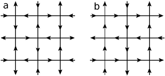
Figure 1: Directed square lattices studied in this paper:(a) F-lattice and (b) Manhattan lattice.

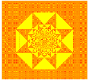
Figure 2: Stable configuration for the ASM, obtained by adding $5\times 10^{4}$ grains at one site, on the F-lattice of Fig.1($a$) with initial chequerboard configuration. Color code: red=0, yellow=1. Apparent orange regions in the picture represent patches with chequerboard configuration. (Details can be seen in the online version using zoom in.)

We also study the effect of having multiple sites of addition on the pattern. For multiple sources, the pattern of small patches near each source is not substantially different from a single-source pattern, but some rearrangement occurs in the larger outer patches. Two patches may sometimes join into one, or conversely, a patch may break up into two. But the number of patches undergoing such changes is finite. However, the sizes of all patches are affected by the presence of other sources, and we show how these changes can be calculated exactly for the asymptotic pattern. Spatial patterns in sandpile models were first discussed by Liu et al liu . The asymptotic shape of the boundaries of sandpile patterns produced by adding grains at single site on different periodic backgrounds was discussed in dhar99 . Borgne borgne obtained bounds on rate of growth of these boundaries and later these bounds are improved by Fey et al redig and Levine et al lionel . The first detailed analysis of different periodic structures found in the patterns are carried out by Ostojic in ostojic . Other special configurations in the ASM models, like the identity borgne ; identity ; caracciolo , or the stable state produced from special unstable states also show complex internal self-similar structures liu , which also share common features with the patterns studied here. There are other models, which are related to the Abelian sandpile model, e.g. the internal Diffusion-Limited Aggregation (DLA), Eulerian walkers (also called rotor-router model), and the infinitely-divisible sandpile, which also show similar structure. For the Internal DLA, Gravner and Quastel showed that the asymptotic shape of the growth pattern is related to the classical Stefan problem in hydrodynamics, and determined the exact radius of the pattern with a single point source gravner . Levine and Peres have studied patterns with multiple sources in these models recently, and proved the existence of a limit shapelevine_peres .

This paper is organized as follows. After defining the model in Section $2$, we discuss scaling of the diameter of the patterns with $N$. We first consider in Section $3$ the pattern in the presence of a line of sink sites. In Section $4$, this analysis is extended to other sink geometries: two intersecting line sinks in two dimensions and two or three intersecting plane sinks in three dimensions. The case of a single sink site is a bit different from others, and is discussed separately in Section $5$. The remaining sections are devoted to a detailed characterization of some of these patterns. In Section $6$ we give a summary of our earlier work on characterization of single source pattern, and use it to characterize the pattern in presence of a line sink. In Section $7$, we discuss the case when there are two sources present. Section $8$ contains a summary and some concluding remarks.

2 Definition of the model

We consider the Abelian sandpile model on the F-lattice (Fig.1$a$). This is a square lattice with directed bonds such that each site has two inward and two outward arrows. A different assignment of arrow directions, that gives us the Manhattan lattice is shown in Fig.1$b$. The asymptotic pattern formed by growing sandpile on the Manhattan lattice is the same as on the F-lattice epl . We shall discuss here only the F-lattice, but the discussion is equally applicable to the Manhattan lattice.

Define a position vector on the lattice, $\mathbf{R}\equiv\left(x,y\right)$. In the Abelian sandpile model, a height variable $z\left(\mathbf{R}\right)$, called the number of grains on the site, is assigned to each site $\mathbf{R}$. In a stable configuration all sites have height $z\left(\mathbf{R}\right)<2$. The system is driven by adding grains at a single site and if this addition makes the system unstable it relaxes by the toppling rule: each unstable site transfers one grain each in the direction of its outward arrows. We start with an initial configuration in which $z\left(\mathbf{R}\right)=1$, for sites with $(x+y)=$ even, and $0$ otherwise. For numerical purpose we used a lattice large enough so that none of the avalanches reaches the boundary. The result of adding $N=5\times 10^{4}$ grains at the origin is shown in Fig.2.

3 Growth of the pattern with line sink

Consider the pattern formed by adding sand grains at a single site in presence of a line of sink sites. Any grain reaching a sink site gets absorbed, and is removed from the system. For simplicity let us consider the source site at $\mathbf{R}_{o}\equiv\left(x_{o},0\right)$ and the sink sites along the $y$-axis. A picture of the pattern produced by adding $14336000$ grains at $\left(1,0\right)$ is shown in Fig.3. When $N$ grains have been added, let $2\Lambda\left(N\right)$ be the diameter of the pattern, measured as the height of the smallest rectangle that enclosed all sites that have toppled at least once. We want to study how $\Lambda(N)$ increases as a function of $N$.

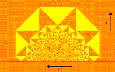
Figure 3: Pattern produced by adding grains at a single site adjacent to a line of sink sites. Color code: red=0 and yellow=1. Apparent orange regions in the picture represent patches with chequerboard configuration. (Zoom in for details in the online version.)

As mentioned before, the pattern exhibits proportionate growth. While there is as yet no rigorous proof of this important property, we assume this in the following. Then, it is natural to describe the pattern in reduced coordinates defined by $\xi=x/\Lambda$ and $\eta=y/\Lambda$. A position vector in this reduced coordinate is defined by $\mathbf{r}=\mathbf{R}/\Lambda\equiv\left(\xi,\eta\right)$. Then in $\Lambda\rightarrow\infty$, the pattern can be characterized by a function $\Delta\rho(\mathbf{r})$ which gives local excess density of sand grains in the pattern in a small rectangle of size $\delta\xi\delta\eta$ about the point $\mathbf{r}$, with $1/\Lambda\ll\delta\xi$, $\delta\eta\ll 1$.

Let $T_{\Lambda}\left(\mathbf{R}\right)$ be the number of toppling at site $\mathbf{R}$ when the diameter reaches value $2\Lambda$ for the first time. Define

$$\phi\left(\mathbf{r}\right)=\lim_{\Lambda\rightarrow\infty}\frac{1}{2\Lambda^{2}}T_{\Lambda}\left(\mathbf{R}^{\prime}\right),$$ (1)

where $\mathbf{R}^{\prime}\equiv\left(\lfloor\Lambda\xi\rfloor,\lfloor\Lambda\eta\rfloor\right)$ with $\lfloor x\rfloor$ being the floor function which gives the largest integer $\leq x$.

From the conservation of sand-grains in the toppling process, it is easy to see that $\phi$ satisfies the Poisson equation epl

$$\nabla^{2}\phi\left(\mathbf{r}\right)=\Delta\rho\left(\mathbf{r}\right)-\frac{N}{\Lambda^{2}}\delta\left(\mathbf{r}-\mathbf{r}_{o}\right)$$ (2)

for all $\mathbf{r}$ in the right-half plane with $\xi>0$, where $\mathbf{r}_{o}$ is the position of the source in reduced coordinates. Also as there are no toppling at sink sites, $\phi$ must satisfy the boundary condition

$$\phi\left(\mathbf{r}\right)=0\rm{~{}~{}for~{}all~{}}\mathbf{r}\equiv\left(0,\eta\right).$$ (3)

A complete information of $\phi\left(\mathbf{r}\right)$ determines the density function $\Delta\rho\left(\mathbf{r}\right)$ and in turn characterizes the asymptotic pattern.

We can think of $\phi$ as the potential due to a point charge $N/\Lambda^{2}$ at $\mathbf{r}_{o}$ and an areal charge density $-\Delta\rho\left(\mathbf{r}\right)$, in presence of a grounded conducting line along the $\eta$-axis. This problem can be solved using the well-known method of images in electrostatics. Let $\mathbf{r}^{\prime}$ be the image point of $\mathbf{r}$ with respect the $\eta$-axis. Define $\Delta\rho\left(\mathbf{r}\right)$ in the left half plane as

$$\Delta\rho\left(\mathbf{r}^{\prime}\right)=-\Delta\rho\left(\mathbf{r}\right).$$ (4)

Then the Poisson equation for this new charge configuration is

$$\nabla^{2}\phi(\mathbf{r})=\Delta\rho(\mathbf{r})-\frac{N}{\Lambda^{2}}\delta\left(\mathbf{r}-\mathbf{r}_{o}\right)+\frac{N}{\Lambda^{2}}\delta\left(\mathbf{r}-\mathbf{r^{\prime}}_{o}\right).$$ (5)

As the function $\Delta\rho\left(\mathbf{r}\right)$ is odd under reflection, $\phi$ automatically vanishes along the $\eta$-axis.

We define $N_{r}$ as the number of sand grains that remain unabsorbed. Then

$$N_{r}=\sum_{x>0}\sum_{y}\Delta z\left(x,y\right),$$ (6)

where $\Delta z\left(x,y\right)$ is the change in height variables before and after the system relaxes. Clearly, for large $\Lambda$, we can write

$$N_{r}\simeq\Lambda^{2}\int_{\mathbb{H}}d\tau\Delta\rho\left(\mathbf{r}\right),$$ (7)

where $d\tau=d\xi d\eta$ is the infinitesimal area around $\mathbf{r}\equiv\left(\xi,\eta\right)$ and the integration performed over the right half-plane $\mathbb{H}$ with $\xi>0$. We shall use the sign $\simeq$ to denote equality up to leading order in $\Lambda$. Since $\Delta\rho\left(\mathbf{r}\right)$ is a non-negative bounded function, exactly zero outside a finite region, this integral exists. Let its value be $C_{2}$ and then we have

$$N_{r}\simeq C_{2}\Lambda^{2}.$$ (8)

Let $N_{a}$ denote the number of grains that are absorbed by the sink sites. Then considering that grains can reach sink sites only by toppling at its neighbors we have

$$N_{a}\simeq\frac{1}{2}\sum_{y}T_{\Lambda}\left(1,y\right).$$ (9)

The factor $1/2$ comes from the fact that in F-lattice, only half of the sites on the column $x=1$ would have arrows going out to the sink sites. Then using our scaling ansatz in equation (1), for $\Lambda$ large,

$$T_{\Lambda}\left(1,y\right)\simeq 2\Lambda\left.\frac{\partial\phi}{\partial\xi}\right\arrowvert_{\xi=0}.$$ (10)

Hence

$$N_{a}\simeq\Lambda^{2}\int_{-\infty}^{\infty}d\eta\left.\frac{\partial\phi}{\partial\xi}\right\arrowvert_{\xi=0}.$$ (11)

Now from equation (5) the potential $\phi$ can be written as sum of two terms: $\phi_{dipole}$ due to two point charges $N/\Lambda^{2}$ and $-N/\Lambda^{2}$ at $\mathbf{r}_{o}\equiv\left(\xi_{o},0\right)$ and its image point $\mathbf{r}^{\prime}_{o}\equiv\left(-\xi_{o},0\right)$ respectively, and the term $\phi_{rest}$ due to the areal charge density.

$$\phi\left(\mathbf{r}\right)=\phi_{dipole}\left(\mathbf{r}\right)+\phi_{rest}\left(\mathbf{r}\right),$$ (12)

where

$$\nabla^{2}\phi_{dipole}\left(\mathbf{r}\right) = -\frac{N}{\Lambda^{2}}\delta\left(\mathbf{r}-\mathbf{r}_{o}\right)+\frac{N}{\Lambda^{2}}\delta\left(\mathbf{r}-\mathbf{r}^{\prime}_{o}\right),$$

$$\nabla^{2}\phi_{rest}\left(\mathbf{r}\right) = \Delta\rho\left(\mathbf{r}\right).$$ (13)

We first consider the case where $R_{o}$ is finite and $r_{o}=R_{o}/\Lambda$ vanishes in the large $\Lambda$ limit. Then $\phi_{dipole}$ reduces to a dipole potential, and it diverges near origin. However, $\phi_{rest}\left(\mathbf{r}\right)$ is a non-singular function for all $\mathbf{r}$. From the solution of dipole potential, it is easy to show that

$$\phi_{dipole}\left(r,\theta\right)\approx A\frac{\cos\theta}{r},$$ (14)

for $1\gg r\gg 1/\Lambda$, where we have used polar coordinates $\left(r,\theta\right)$ with $\theta$ being measured with respect to the $\xi$-axis. Here $A$ is a numerical constant, which is determined by the property of the asymptotic pattern. Then

$$\left.\frac{\partial\phi}{\partial\xi}\right\arrowvert_{\xi=0}=\frac{A}{\eta^{2}},$$ (15)

and the integral in equation (11) diverges as $A/\eta_{min}$, where $\eta_{min}$ is the cutoff introduced by the lattice. Using $\eta_{min}=\mathcal{O}\left(1/\Lambda\right)$ it is easy to show that

$$N_{a}\simeq C_{1}\Lambda^{3},$$ (16)

where $C_{1}$ is a constant. Then using equation (8) and (16) and that $N_{a}$ and $N_{r}$ add up to $N$, we get

$$C_{1}\Lambda^{3}+C_{2}\Lambda^{2}\doteqdot N.$$ (17)

Here we use the symbol $\doteqdot$ to denote “nearly equal to”. Considering the dominant term in the expression for large $\Lambda$, it follows that $\Lambda$ increases as $N^{1/3}$.

The above scaling behavior is verified with our numerical data. Let $\Lambda^{\ast}\left(N\right)$ be the real positive root of the equation (17) for a given value of integer $N$. As $\Lambda$ takes only integer values on the lattice, an estimate of it would be $Nint\left[\Lambda^{\ast}(N)\right]$ the integer nearest to $\Lambda^{\ast}\left(N\right)$.

Interestingly, we found that for a choice of $C_{1}=0.1853$ and $C_{2}=0.528$, this estimate gives values which differ from the measured value $\Lambda\left(N\right)$ at most by $1$ for all $N$ in the range of $100$ to $3\times 10^{6}$. Clearly more precise estimates of $C_{1}$ and $C_{2}$ would be required if we want this to work for larger $N$. Here we find Eqs.(8) and (16) on dimensional counting grounds, and the final Eq.(17) is then only a statement of conservation of sand grains. It is quite remarkable that this scaling analysis gives almost the exact value of $\Lambda\left(N\right)$. The equation has an important feature. It includes “correction to scaling” term whereas the usual scaling analysis ignores the sub-leading powers.

For patterns in the other limit where the source is placed at a distance $\mathcal{O}\left(\Lambda\right)$ such that $r_{o}$ is non zero for $\Lambda\rightarrow\infty$, $\phi_{dipole}$ is non-singular along the sink line. Then, clearly $N_{a}\sim\Lambda^{2}$ and as a result $\Lambda\left(N\right)\sim N^{1/2}$.

4 Generalization to more complex patterns

The above analysis can be easily generalized to a case with sink sites along two straight lines intersecting at an angle $\omega$ and a point source inside the wedge. For square lattice, $\omega=0,\pi/2,\pi,3\pi/2$ and $2\pi$ are most easily constructed, and avoid problems of lines with irrational slopes, or slopes of rational numbers with large denominators. The wedge with wedge-angle $\omega=\pi/2$ is obtained by placing sink sites along the $x$ and $y$-axis and the source site at $\mathbf{R}_{o}\equiv\left(1,1\right)$ in the first quadrant. The pattern with line sink, discussed in previous section, correspond to $\omega=\pi$.

For any general $\omega$, corresponding electrostatic problem reduces to determining the potential function $\phi$ inside a wedge formed by two intersecting grounded conducting lines. Again the potential has two contributions: the potential $\phi_{point}\left(\mathbf{r}\right)$ due to a point charge at the source site and the potential $\phi_{rest}\left(\mathbf{r}\right)$ due to the areal charge density. We first consider the case where the source site is placed at a finite distance from the wedge corner such that the distance in reduced coordinate vanishes for $\Lambda$ large limit. In this limit $\phi_{rest}$ is non-singular function of $\mathbf{r}$ while $\phi_{point}$ diverges close to the origin. A simple calculation of the electrostatic problem gives

$$\phi_{point}\left(r,\theta\right)=A\frac{\sin\alpha\theta}{r^{\alpha}},$$ (18)

where $\alpha=\pi/\omega$ and we have used polar coordinates $\left(r,\theta\right)$ with the polar angle $\theta$ measured from one of the absorbing lines. Again $A$ is a constant independent of $N$ or $\Lambda$ and is a property of the asymptotic pattern. Then arguing as before, we get

$$N_{a}\simeq C_{1}\Lambda^{2+\alpha}\rm{~{}~{}and~{}~{}}N_{r}\simeq C_{2}\Lambda^{2}.$$ (19)

So the equation analogous to equation (17) is

$$C_{1}\Lambda^{2+\alpha}+C_{2}\Lambda^{2}\doteqdot N.$$ (20)

For wedge angle $\omega=\pi$, $\alpha=1$, and the above equation reduces to Eq.(17). For $\omega=2\pi$, the value of $\alpha$ is $1/2$. Again, Eq. (20) is in very good agreement with our numerical data. Let $\Lambda^{\ast}(N)$ be the solution of Eq. (20) for a given $N$. Choosing $C_{1}=0.863408$ and $C_{2}=0.043311$, we find that the function $Nint\left[\Lambda^{\ast}\left(N\right)\right]$ differ from the measured values of $\Lambda$ at most by $1$ for all $N$ in the range from $100$ to $2\times 10^{5}$.

For the problem where the source site is at a distance $\mathcal{O}\left(\Lambda\right)$ from the wedge corner both the functions $\phi_{rest}$ and $\phi_{point}$ are nonsingular close to the origin. Then it is easy to show that $\Lambda\left(N\right)$ grows as $N^{1/2}$.

The argument is easily extended to other lattices with different initial height distributions, or to higher dimensions. Consider, for example, an Abelian sandpile model defined on the cubic lattice. Allowed heights are $0$ to $5$, and a site topples if the height exceeds $5$, and sends one particle to each neighbor. The sites are labelled by the Cartesian coordinates $(x,y,z)$, where $x,y$ and $z$ are integers. We consider the infinite octant defined by $x\geq 0,y\geq 0,z\geq 0$. We start with all heights $4$, and add sand grains at the site $(1,1,1)$. We assume that the sites on planes $x=0$, $y=0$ and $z=0$ are all sink sites, and any grain reaching there is lost. We add $N$ grains and determine the diameter of the resulting stable pattern.

We again reduce the potential function in two parts: $\phi_{point}$ due to a point charge at $\left(1/\Lambda,1/\Lambda,1/\Lambda\right)$ and $\phi_{rest}$ due to bulk charge density in presence of three conducting grounded planes. Then simple electrostatic calculation gives that the potential $\phi_{point}$ is the octapolar potential of the form

$$\phi\left(r,\theta,\Phi\right)\simeq\frac{f\left(\theta,\phi\right)}{r^{4}},$$ (21)

where the spherical coordinate is used to denote position. This then implies that the equation determining the dependence of $\Lambda$ on $N$ is

$$C_{1}\Lambda^{6}+C_{2}\Lambda^{3}\doteqdot N$$ (22)

Like the other cases, this relation is also confirmed against numerical data. The function $Nint\left[\Lambda^{\ast}\left(N\right)\right]$ with $C_{1}=0.0159$ and $C_{2}=88$ gives almost exact values of $\Lambda\left(N\right)$. We have checked for $N$ between $5\times 10^{5}$ to $5\times 10^{8}$, the difference is at most $1$.

5 A single sink site

Let the site of addition is the origin and the sink site is placed at $\mathbf{R}_{o}$. We will show that when $\mathbf{r}_{o}$ lies in a dense patch (color yellow in Fig.4), the asymptotic patterns are identical to the one produced in absence of a sink.

The patterns produced for $r_{o}$ close to $1$ with sink sites placed deep inside a dense patch is simple to analyze, even for finite but large $\Lambda$. One such pattern is presented in Fig.4.

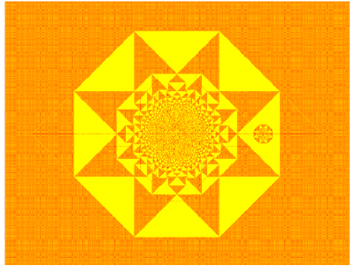
Figure 4: Pattern produced by adding $224000$ grains at the origin with a sink site at $\left(400,0\right)$ inside a patch of density $1$ (color yellow ). Color code red$=0$ and yellow$=1$. The apparent orange regions correspond to chequerboard height distribution. (Zoom in for details in the online version.)

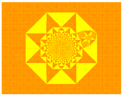
Figure 5: Pattern produced by adding $224000$ grains at origin with a sink site placed at $\left(360,140\right)$ inside a low density patch. Color code red$=0$ and yellow$=1$. The apparent orange regions correspond to the chequerboard height distribution. (Details can be seen in the online version using zoom in.)

We see that the effect of sink site on the pattern is to produce a depletion pattern centered at the sink site. The depletion pattern is a smaller copy of the single source pattern. We define the function $\Delta z_{sink}\left(\mathbf{R};N\right)$ as the difference between the heights at ${\mathbf{R}}$ in the final stable configuration produced by adding $N$ grains at the origin, with and without sink.

$$\Delta z_{sink}\left(\mathbf{R};N\right)=\Delta z_{source+sink}\left({\mathbf{R}};N\right)-\Delta z_{source}\left(\mathbf{R};N\right).$$ (23)

From the figure it is seen that, in this case, $\Delta z_{sink}\left(\mathbf{R};N\right)$ is negative of the pattern produced by a smaller source, centered at $\mathbf{R}_{0}$. The number of particles required to produce this smaller pattern is exactly the number of particles $N_{a}$ absorbed at the sink site.

$$\Delta z_{sink}\left(\mathbf{R};N\right)=-\Delta z_{source}\left(\mathbf{R}-\mathbf{R}_{o};N_{a}\right).$$ (24)

This is immediately seen from the fact that the toppling function $T_{\Lambda}\left(\mathbf{R}\right)$ satisfies

$$\sum_{\mathbf{R^{\prime}}\in\Gamma(\mathbf{R})}T_{\Lambda}\left(\mathbf{R^{\prime}}\right)-2T_{\Lambda}\left(\mathbf{R}\right)=\Delta z_{source+sink}\left(\mathbf{R};N\right)-N\delta_{\mathbf{R},\mathbf{0}}+N_{a}\delta_{\mathbf{R},\mathbf{R}_{o}},$$ (25)

where $\Gamma(\mathbf{R})$ is the set of two neighbors which transfer grains to the site $\mathbf{R}$ under toppling. Let $T_{source}({\mathbf{R}};N)$ be the number of toppling at ${\mathbf{R}}$, when we add $N$ particles at the origin. Since Eq. (25) is a linear equation, it follows that a solution of this equation is

$$T_{\Lambda}\left(\mathbf{R}\right)=T_{source}\left(\mathbf{R};N\right)-T_{source}\left(\mathbf{R}-\mathbf{R}_{o};N_{a}\right),$$ (26)

This is a valid solution of our problem, if the corresponding heights in the final configuration with sink are all non-negative. This happens when the region with nonzero $\Delta z_{sink}$ is confined within the dense patch.

The number $N_{a}$ can be determined from the requirement that number of toppling at the sink site is zero. The potential function for a single source problem diverges as $\left(4\pi\right)^{-1}\log r$ near the source epl . Considering the ultra violate cutoff due to lattice, $T_{source}\left(\mathbf{R},N\right)$ at $\mathbf{R}=0$ can be approximated by $\left(4\pi\right)^{-1}N\log N$ in leading orders in $N$. Then at $\mathbf{R}=\mathbf{R}_{0}$, $T_{source}\left(\mathbf{R}-\mathbf{R}_{o};N_{a}\right)$ is approximately equal to $(4\pi)^{-1}N_{a}\log N_{a}$ whereas $T_{source}\left(\mathbf{R}_{0};N\right)\approx N\phi_{source}(\mathbf{r}_{0})$, where $\phi_{source}\left(\mathbf{r}\right)$ is the potential function for the problem without a sink. Then from equation (26) we have

$$\frac{1}{4\pi}N_{a}\log N_{a}\simeq N\phi_{source}\left(\mathbf{r}_{o}\right).$$ (27)

For large $N$, this implies that $N_{a}\simeq 4\pi\phi_{source}\left(\mathbf{r}_{o}\right)N/\log N$. In numerical measurement it is found that for a change of $N$ from $224000$ to $896000$, $N_{a}\log{N}/N$ changes by less than $7\%$ which is consistent with the above scaling relation. For large $N$, for a sink at a fixed reduced coordinate $\mathbf{r}_{o}$, the relative size of the defect produced by the sink decreases as $(\log N)^{-1/2}$. Hence asymptotically, the fractional area of the defect region will decrease to zero, if sink position $\mathbf{r}_{o}$ is in a dense patch.

When the sink site is inside a light patch, the subtraction procedure of equation (24) gives positive heights, and no longer gives the correct solution. However it is observed for patches in the outer layer where patches are large, effect of sink site is confined within neighboring dense patches (Fig.5) and rest of the pattern in the asymptotic limit remains unaffected.

The pattern where the source and sink sites are adjacent to each other appears to be very similar to the one produced in absence of sink site. This is easy to see. The Poisson equation analogous to equation (5) for this problem is

$$\nabla^{2}\phi(\mathbf{r})=\Delta\rho(\mathbf{r})-\frac{N}{\Lambda^{2}}\delta(\mathbf{r})+\frac{N_{a}}{\Lambda^{2}}\delta(\mathbf{r}-\mathbf{r}_{o}),$$ (28)

where $N_{a}$ is the number of grains absorbed in the sink site at $\mathbf{r}_{o}$. In an electrostatic analogy, as discussed earlier, $\phi$ can be considered as the potential due to a distributed charge of density $-\Delta\rho\left(\mathbf{r}_{o}\right)$ and two point charges of strength $N/\Lambda^{2}$ and $-N_{a}/\Lambda^{2}$ placed at origin and at $\mathbf{r}_{o}$ respectively. It is easy to see that the dominant contribution in the potential is the monopole term with net charge $(N-N_{a})/\Lambda^{2}$. The contribution due to other terms decreases as $1/\Lambda$ for large $\Lambda$, and the asymptotic pattern is the same as without a sink, with $N-N_{a}$ particles added.

The number of particles absorbed $N_{a}$ is determined by the condition that the number of toppling at $(1,0)$ ( the sink position) is zero. The potential produced by the areal charge density at $(1,0)$ and $(0,0)$ is nearly the same. The number of toppling at $(1,0)$ if we add $N_{a}$ particles at the sink site is approximately $\left(4\pi\right)^{-1}N_{a}\log N_{a}$. Now, from the solution of the discrete Laplacian, the number of toppling produced at $(1,0)$ due to $N$ particles added at $(0,0)$ is approximately $\left(4\pi\right)^{-1}\left(N\log N-CN\right)$ with $C$ being an undetermined constant. Equating these two, we get

$$N_{a}\log N_{a}\doteqdot N\log N-CN$$ (29)

The above relation is verified with numerical data in figure 6. We find that $(N\log N-N_{a}\log N_{a})/N$ asymptotically approaches a value $C=2.155$ with the difference from the asymptotic value decreasing as $N^{-1/2}$. As the asymptotic pattern is the same as produced by adding $\left(N-N_{a}\right)$ grains at the origin without a sink, we have $N-N_{a}\simeq\Lambda^{2}$. Then, using the numerical value for $C$ we get

$$(N-\Lambda^{2})\log(N-\Lambda^{2})\doteqdot N\log N-2.155N.$$ (30)

Simplification of this equation for large $N$, shows that $\Lambda$ grows as $\sqrt{N/\log N}$ with $N$.

For finite $\Lambda$, the leading correction to $\phi\left(\mathbf{r}\right)$ comes from the dipole term in the potential. Presence of this term breaks the reflection symmetry of the pattern about the origin. The relative contribution of the dipole potential compared to the monopole term decays as $\log\Lambda/\Lambda$. A measure of the bilateral asymmetry is the difference of boundary distances on two opposite sides of the source. This difference is plotted in Fig.7, where $R_{1}$ and $R_{2}$ are boundary distances measured along the positive and negative $x$ axis with a sink site placed at $\left(1,0\right)$. The difference $(R_{2}-R_{1})$ is found to fit to $1.22\log{(R_{2}+0.5)}$.

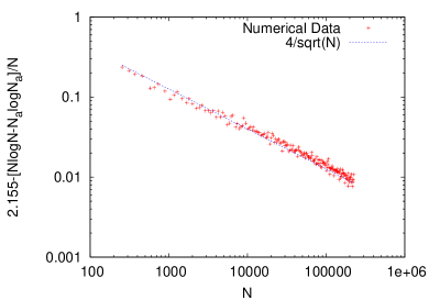
Figure 6: Dependence of number of absorbed grains $N_{a}$ on number of grains added $N$ at the origin with a sink site at $\left(1,0\right)$.

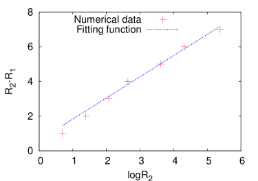
Figure 7: Bilateral asymmetry due to the presence of a sink site in Fig.4.

6 Characterization of the pattern with line sink

We start by recalling the characterization of single source pattern epl . As discussed in Section $3$, the asymptotic patterns can be characterized by the function $\Delta\rho\left(\mathbf{r}\right)$ in rescaled coordinate. The single source pattern on F-lattice with chequerboard background is made of union of distinct regions, called “patches”, where inside each patch $\Delta\rho\left(\mathbf{r}\right)$ is constant and takes only two possible values, $1/2$ in a dense patch and $0$ in a light patch epl .

The potential function $\phi\left(\mathbf{r}\right)$ for the single source problem follows the Poisson equation

$$\nabla^{2}\phi(\mathbf{r})=\Delta\rho(\mathbf{r})-\frac{N}{\Lambda^{2}}\delta(\mathbf{r}).$$ (31)

The condition that determines $\phi\left(\mathbf{r}\right)$ is the requirement that inside each patch of constant density, it is a quadratic function of $\xi$ and $\eta$ epl . Let us write

$$\phi\left(\mathbf{r}\right)=a\xi^{2}+2h\xi\eta+b\eta^{2}+d\xi+e\eta+f$$ (32)

where $a$, $h$, $b$, $d$, $e$ and $f$ are constants inside a patch and $a+b=\Delta\rho/2$ corresponding to the patch. Then each patch is characterized by these parameters. Continuity of $\phi\left(\mathbf{r}\right)$ and its derivatives along the boundary between two adjacent patches imposes linear relations among the corresponding parameters. These linear equations can be solved on the connectivity graph of patches which forms a square lattice on two sheeted Riemann surface epl .

The pattern with line sink (Fig.3) retained two important properties present in the single source pattern. These are: the asymptotic pattern is made of union of two types of patches of excess density $1/2$ and $0$ and the separating boundaries of patches are straight lines of slope $0$, $\pm 1$ or $\infty$. However the adjacency graph is changed significantly and this changes the sizes of patches as well. In this section we show how to explicitly determine the potential function on this adjacency graph.

The adjacency graph of the patches is given in Fig.9. This representation of the graph is easier to see by taking $1/r^{3}$ transformation of the pattern and then joining the neighboring patches by straight lines (Fig.8). Each vertex in the graph is connected to four neighbors except the vertices corresponding to the patches next to the absorbing line. These have coordination number $3$. Also the vertex at the center corresponding to the exterior of the pattern is connected to seven neighbors.

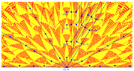
Figure 8: $1/r^{3}$ transformation of the pattern in Fig.3. Two adjoining patches are connected by drawing a straight line.

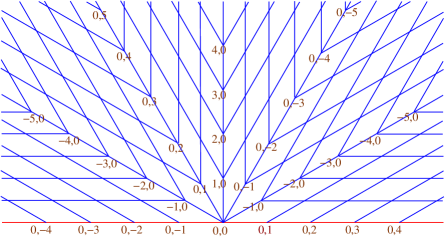
Figure 9: Adjacency graph of the patches in pattern in Fig.3.

Let us write the quadratic potential function in a patch $P$ having excess density $1/2$ as

$$\phi_{{}_{P}}(\mathbf{r})=\frac{1}{8}(m_{{}_{P}}+1)\xi^{2}+\frac{1}{4}n_{{}_{P}}\xi\eta+\frac{1}{8}(1-m_{{}_{P}})\eta^{2}+d_{{}_{P}}\xi+e_{{}_{P}}\eta+f_{{}_{P}},$$ (33)

where the parameters $m$, $n$, $d$, $e$ and $f$ take constant values within a patch. Similarly for the lighter patches $P^{\prime}$

$$\phi_{{}_{P^{\prime}}}(\mathbf{r})=\frac{1}{8}m_{{}_{P^{\prime}}}(\xi^{2}-\eta^{2})+\frac{1}{4}n_{{}_{P^{\prime}}}\xi\eta+d_{{}_{P^{\prime}}}\xi+e_{{}_{P^{\prime}}}\eta+f_{{}_{P^{\prime}}}.$$ (34)

Using the continuity of $\phi\left(\mathbf{r}\right)$ and its derivatives along the common boundaries between neighboring patches it has been shown that for single source pattern without sink sites $m$ and $n$ take integer values epl . Same arguments also applies for this problem and $\left(m,n\right)$ are the coordinates of the patches in the adjacency graph in Fig.9. These coordinates are shown next to some of the vertices.

There are two different patches corresponding to same set of $\left(m,n\right)$ values. Infact, as in the single source pattern the adjacency graph forms a square lattice on two sheeted Riemann surface, the same is formed for this pattern but on a three sheeted Riemann surface. The pattern covers half of the surface with $\left(m,n\right)$ being the Cartesian coordinates on the surface.

Define function $D\left(m,n\right)=d\left(m,n\right)+ie\left(m,n\right)$ on this lattice. Using the matching conditions along the common boundaries between neighboring patches it can be shown that $d$ and $e$ satisfy discrete Cauchy-Riemann condition epl

$$d\left(m+1,n+1\right)-d\left(m,n\right) = e\left(m,n+1\right)-e\left(m+1,n\right),$$

$$e\left(m+1,n+1\right)-e\left(m,n\right) = d\left(m+1,n\right)-d\left(m,n+1\right),$$ (35)

and then the function $D$ follows discrete Laplaces equation

$$\sum_{i=\pm 1}\sum_{j=\pm 1}D(m+i,n+j)-4D(m,n)=0,$$ (36)

on this adjacency graph. Let us define $M=m+in$ and $z=\xi+\eta$. Then, as argued before, close to the origin the potential $\phi$ diverges as $1/r$ (equation (14)). Then the corresponding complex potential $\Phi\left(z\right)\sim 1/z$. As $M\sim{d^{2}\Phi}/{dz^{2}}$, and $D\sim d\Phi/dz$, it follows that for large $|m|+|n|$,

$$D\sim M^{2/3}.$$ (37)

The condition that on the absorbing line $\phi\left(\mathbf{r}\right)$ must vanish implies that for the vertices with even $n$ along the red line in Fig.9 $e(0,n)$ vanishes. These vertices correspond to the patches with absorbing line as horizontal boundary in Fig.3. Equation (36) with above constraint and the boundary condition in equation(37) has a unique solution. The normalization of $\phi$ is fixed by the requirement that $d(1,0)=-1$ which fixes the diameter of the pattern to be $2$ in reduced units.

Equation 36 is the standard two-dimensional lattice Laplace equation, whose solution is well-known when $\left(m,n\right)\in\mathbb{Z}^{2}$ spitzer . In our case when the lattice sites form a surface of two sheets, we have not been able to find a closed-form formula for $D(m,n)$. However the solution can be determined numerically to very good precision by solving it on a finite grid $-L\leq m,n\leq L$ with the above conditions imposed exactly at the boundary. The calculation is performed with $D=M^{2/3}$ at the boundary and then the solution is normalized to have $d\left(1,0\right)=-1$. We determined $d$ and $e$ numerically for $L=100$, $200$, $300$, $400$ and $500$ and extrapolated our results for $L\rightarrow\infty$.

Comparison of results from this numerical calculation and that obtained by measurements on the pattern is presented in Table $1$. We considered four different lengths $R_{1}$, $R_{2}$, $R_{3}$ and $R_{4}$ on the pattern and they are shown in Fig.10. Among them, according to the definition of the diameter of the pattern, $R_{1}=2\Lambda$. We present values of $R_{2}$, $R_{3}$ and $R_{4}$ normalized by $R_{1}$ for different $N$. Theoretical values of these lengths are determined from asymptotic values of $d$ and $e$. Comparision of these results shows very good agreement among the theoretical and measured values.

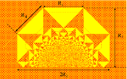
Figure 10: Spatial lengths $R_{1}$, $R_{2}$, $R_{3}$ and $R_{4}$ tabulated in Table $1$.

N	$896k$	$14336k$	$57344k$	$229376k$	Theoretical
$\frac{R_{2}}{R_{1}}$	0.769	0.768	0.770	0.770	0.7698
$\frac{R_{3}}{R_{1}}$	0.675	0.675	0.667	0.668	0.6666
$\frac{R_{4}}{R_{1}}$	0.609	0.609	0.617	0.616	0.6172

Table 1: Comparison of different lengths measured directly from the pattern in Fig.10 for increasing values of $N$, with their theoretical values.

7 Patterns with two sources

In this section we discuss patterns produced by adding $N$ grains each at two sites placed at a distance $2\Lambda\mathbf{r_{o}}$ from each other along the $x$-axis at $\Lambda\mathbf{r}_{o}$ and $-\Lambda\mathbf{r}_{o}$ with $\mathbf{r}_{o}\equiv\left(\xi_{o},0\right)$. Again the diameter $2\Lambda$ is defined as the height of the smallest rectangle enclosing all sites that have toppled atleast once. Two limits $r_{0}$ close to zero and $r_{0}$ large are trivial: For $r_{o}\rightarrow 0$, the asymptotic pattern is same as that produced by adding grains at a single site. On the otherhand if $r_{o}>1$, each source produces its own pattern, which do not overlap, and the final pattern is simple superposition of the two patterns.

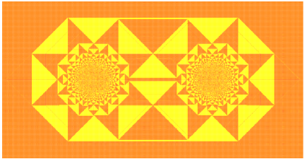
Figure 11: Pattern produced by adding $N=640000$ grains each at ($-760,0$) and ($760,0$) on F-lattice with initial chequerboard distribution of grains and relaxing. This corresponds to $r_{o}=0.95$. Color code red=0 and yellow=1. (Details can be seen in the online version using zoom in )

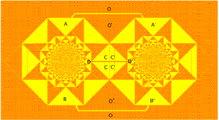
Figure 12: Pattern constructed by combining two single source patterns and drawing connecting lines between few patches following the connectivity in the pattern in Fig.11.

As noted before, the connectivity graph for single source pattern has square lattice structure on a Riemann surface of two sheets epl . Then the graph for two non-intersecting single source pattern is square lattice on two disjoint Riemann surfaces each consists of two sheets (Fig.13). Only the vertex at the origin represent the exterior of the pattern, which is same for both the single source patterns. It has sixteen neighbors and is placed midway between the two Riemann surfaces. For later convenience let us associate the lower Riemann surface to the pattern around $-\mathbf{r}_{o}$ and denote it by $\Gamma_{L}$. Similarly the upper Riemann surface as $\Gamma_{R}$ corresponding to the pattern around $\mathbf{r}_{o}$.

For $0<r_{o}<1$, using the Abelian property, we can first topple as if the other source was absent. The resulting pattern still has some unstable sites in the region where the patterns overlap. Further relaxing these sites transfers these excess grains outward, and changes the dimensions and positions of patches: some patches become bigger, some may merge, and some times a patch may beak into two disjoint patches.

The pattern produced with two sources with $r_{0}=0.95$ is shown in Fig.11. We see that there are still only two types of periodic patches, corresponding to $\Delta\rho(\mathbf{r})$ values $0$ and $1/2$, and the slopes of the boundaries between patches takes values $0$, $\pm 1$ or $\infty$.

The relaxations due to overlaps change the adjacency graph from the case with no overlap. This modified adjacency graph is shown in Fig.14. However, for $r_{0}$ just below $1$, these changes are few, and are listed below.

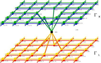
Figure 13: Representation of adjacency graph of patches for two non-overlapping single source patterns as square grid on two Riemann surfaces each of two sheets. Vertices with the same $(m,n)$ coordinates on different sheets are represented by different colors.

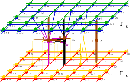
Figure 14: Connectivity graph for two intersecting single source patterns around two sites of addition placed at a distance $2\mathbf{r}_{o}$ from each other. The graph has the structure of square grids on four Riemann sheets except for a finite number of vertices indicated by alphabates $A$, $B$, $O$, $O^{\prime}$, $O"$ and $D$ shown placed in middle layer. This graph remains unchanged for $r_{o}$ in the range $0.65$ to $1.00$.

i) We note that patches labelled $A$ and $A^{\prime}$ in Fig.12 have the same potential function $\phi$. Then, for $r_{0}$ just below $1$, these patterns can join with each other by a thin strip. This only requires a small movement in the boundaries of nearby patches, ( i.e. only a small change in the $d$ and $e$ values of nearby patches). Thus, in the adjacency graph, the vertices corresponding to $A$ and $A^{\prime}$ are collapsed into a single vertex $A$ in Fig.14.

ii) Similarly, the vertices corresponding to patches $B$ and $B^{\prime}$ in Fig.12 are collapsed into a single vertex $B$ in Fig.14.

iii) This divides the region outside the pattern in three parts, $O$, $O^{\prime}$ and $O"$. They are also shown in Fig.14 as separate vertices.

iv) The patches marked $C$ and $C^{\prime}$ also have the same quadratic form, and the vertical boundary between them disappears. However, the patches $D$ and $D^{\prime}$ are also joined by a thin strip. This horizontal strip divides the joined $C$ and $C^{\prime}$ into two again (Fig.12).

The adjacency of other patches remains unchanged. The adjacency graph of the pattern is shown in Fig.14. Interestingly, this new adjacency graph remains the same for all $0.70<r_{0}<1$, even though for $r_{o}<0.85$, the sizes of different patches are substantially different. [Compare the pattern for $r_{0}=0.70$ in Fig.15, with pattern for $r_{0}=0.95$ in Fig.11]. Shape of the patches near the center of Fig.15 is different from that in Fig.11.

In Fig.14, we have have placed the vertices which are formed by merging or dividing patches in the overlap region midway between the Riemann sheets corresponding to the two sources. As $r_{0}$ is decreased below $0.70$, more collisions between growing patches will occur, and the number of vertices in this middle region will increase. For any nonzero $r_{0}$, the number of vertices in the middle layer is finite. In the $r_{o}\rightarrow 0$ limit vertices from both the surfaces $\Gamma_{L}$ and $\Gamma_{R}$ come together and form a single Riemann surface corresponding to a single source pattern around $\mathbf{r}=0$. For $r_{0}$ small, but greater than zero, the outer patches are arranged as in the single-source case, but closer to the sources, one has a crowded pattern near each source. In the adjacency graph, this corresponds to vertices near the patch $(0,0)$ roughly arranged as on a Riemann surface of two sheets, while the ones farther from the patch $(0,0)$ remain undisturbed on the 4-sheeted Riemann surface.

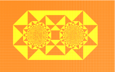
Figure 15: Pattern produced by adding $640000$ grains at site $\left(-600,0\right)$ and $\left(600,0\right)$. Although the pattern is significantly different from the one in Fig.11, their adjacency graph is same.

We now characterize the pattern with two sources, and $r_{0}>0.70$ in detail by explicitly determining the potential function on this adjacency graph.

The Poisson equation analogous to Eq.(31) for this problem is

$$\nabla^{2}\phi(\mathbf{r})=\Delta\rho(\mathbf{r})-\frac{N}{\Lambda^{2}}\delta(\mathbf{r}-\mathbf{r}_{o})-\frac{N}{\Lambda^{2}}\delta(\mathbf{r}+\mathbf{r}_{o}).$$ (38)

Let us use the same quadratic form of the potential function given in equation (33) and equation (34).

Again using the same argument given in epl it can be shown that $m$ and $n$ are the coordinates of the patches in both the adjacency graphs in Fig.13 and Fig.14. These coordinates are shown next to each vertex. Also, in the region away from the origin, on each sheet,the function $D(m,n)=d(m,n)+ie(m,n)$ satisfies the discrete Laplace equation

$$\sum_{i=\pm 1}\sum_{j=\pm 1}D(m+i,n+j)-4D(m,n)=0.$$ (39)

Let us define $z_{o}=\xi_{o}+i\eta_{o}$ where $(\xi_{o},\eta_{o})$ and $(-\xi_{o},-\eta_{o})$ are the coordinates corresponding to $\mathbf{r}_{o}$ and $-\mathbf{r}_{o}$. Considering that close to $\mathbf{r}_{o}$ and $-\mathbf{r}_{o}$ the potential $\phi\left(\mathbf{r}\right)$ diverges logarithmically it can be shown (as done for single source pattern in epl ) that for large $|m|+|n|$,

$$D(m,n) = \pm\frac{A}{\sqrt{2\pi}}\sqrt{M}+\bar{z}_{o}\frac{M}{4}\rm{,~{}on~{}}\Gamma_{L}$$ (40)

$$= \pm\frac{A}{\sqrt{2\pi}}\sqrt{M}-\bar{z}_{o}\frac{M}{4}\rm{,~{}on~{}}\Gamma_{R}$$

where $A$ is a constant independent of $N$ or $\Lambda$.

Again we determine the solution of equation (39) numerically to very good precision by solving it on finite grid $-L\leq m,n\leq L$ with the conditions Eq. (40) imposed exactly at the boundary. The value of $A$ is determined from a self consistency condition that the diameter of the pattern in reduced coordinate is 2 which imposes $2e(-1,0)=-1$ corresponding to the vertex $A$ in Fig.14. We determined $d$ and $e$ numerically for $L=100$, $200$, $300$, $400$ and $500$ and extrapolated our results for $L\rightarrow\infty$.

Comparison of results from this numerical calculation and that obtained by measurements on the pattern in presented in Table $2$. We considered five different lengths in the pattern corresponding to $r_{o}=0.800$. These different lengths are drawn in Fig.16 and their values rescaled by $\sqrt{N}$, for the patterns with increasing $N$, is given in Table $2$. Theoretical results are obtained using the asymptotic values of $d$ and $e$ for large $L$. The rescaled lengths extrapolated to infinite $N$ limit matches very well to the theoretical results.

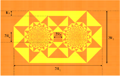
Figure 16: Spatial lengths $R_{1}$, $R_{2}$, $R_{3}$, $R_{4}$ and $R_{5}$ tabulated in Table.$2$

N	$2.5k$	$10k$	$40k$	$160k$	$640k$	Theoretical
$\frac{R_{1}}{\sqrt{N}}$	1.84	1.84	1.84	1.83	1.83	1.82
$\frac{R_{2}}{\sqrt{N}}$	1.06	1.07	1.07	1.06	1.05	1.06
$\frac{R_{3}}{\sqrt{N}}$	0.22	0.21	0.20	0.19	0.18	0.18
$\frac{R_{4}}{\sqrt{N}}$	0.18	0.19	0.19	0.18	0.18	0.18
$\frac{R_{5}}{\sqrt{N}}$	0.20	0.22	0.21	0.21	0.21	0.21

Table 2: Comparison of different lengths measured directly from the two source pattern for $r_{o}=0.800$ with their theoretical values.

8 Summary

We have shown that exact characterization of the patterns in F-lattice on chequerboard background reduces to solving a discrete Laplace equation on the adjacency graph of the pattern. For the single source pattern this graph is a square grid on two-sheeted Riemann surface and in presence of a line sink it is on a $3$-sheeted Riemann surface. This Riemann surface structure occurs for other sink geometries also and the number of sheets can be determined from the way $\phi$ diverges near origin.

If the potential $\phi(r)$ diverges as $r^{-a}$ near the origin, then the corresponding complex function $\Phi(z)\sim z^{-a}$. Then $\frac{d^{2}}{dz^{2}}\Phi\sim z^{-2-a}$. In all the cases we studied above, the patch to which point $z$ belongs is characterized by integers $(m,n)$, where $\frac{d^{2}}{dz^{2}}\Phi\sim m+in$. Also $\frac{d}{dz}\Phi\sim d+ie$. Writing $D=d+ie$, and $M=m+in$, we see that $D\sim M^{\frac{1+a}{2+a}}$. This then gives the number of Riemann sheets. For example, for a wedge angle $\omega=2\pi$, we have $a=1/2$. Then $D\sim M^{3/5}$, and the Riemann surface would have 5 sheets.

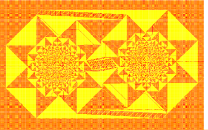
Figure 17: Pattern produced by adding $N=40000$ grains each at ($-180,0$) and ($180,20$) on F-lattice with initial chequerboard distribution of grains and relaxing. Color code red=0 and yellow=1. (Details can be seen in the online version using zoom in )

The cases where the full pattern can be explicitly determined are clearly special. For example, one of the conditions used for exact characterization of patterns in this paper is that inside each patch the height variables are periodic and hence $\Delta\rho\left(\mathbf{r}\right)$ is constant. It is easy to check that this condition is not met for most of the sink geometries. For example, patterns of the type discussed in Section $4$ with any $\omega$ other than integer multiples of $\pi/4$ has aperiodic patches. Similarly for the patterns with two sources even slight deviation of the position of the second source in Fig.11 from the x-axis introduces aperiodic patches. One of such patterns produced by adding $40000$ grains each at $\left(-180,0\right)$ and $\left(180,20\right)$ is shown in Fig.17. The regions with stipes of red and yellow are the aperiodic patches. Also boundary of all these aperiodic patches have slopes other than $0$, $\pm 1$ and $\infty$ and some boundaries of patches are not straight lines. In such cases, the present treatment is clearly not applicable. However the scaling analysis for the growth of spatial lengths in the pattern with $N$ is still valid.

The function $D=d+ie$ satisfies discrete Cauchy-Riemann condition (equation (35)). These functions are known as discrete holomorphic functions in the mathematics literature. They have been usually studied for a square grid of points on the plane duffin ; spitzer . While more general discretizations of the plane have been discussed mercat ; laszlo , not much is known about the behavior of such functions for muti-sheeted Riemann surfaces.

In our analysis we have also used a fact that the patterns have non-zero average overall excess density ( i.e. $C_{2}$ in Eq. (8) is nonzero). The case when $C_{2}$ is zero is quite different, and requires a substantially different treatment. We hope to discuss such patterns in a future publication next .

- (1) Schulman L. S. and Seidon P. E.: Statistical Mechanics of a Dynamical System Based on Conway’s Game of Life. J. Stat. Phys.19, 293 (1978) .
- (2) Pearson J. E.: Complex Patterns in a Simple System. Science 261, 189 (1993).
- (3) A particular mathematical model is discussed in Hadeler K. P. and Kuttler C.: Dynamical Models for Granular Matter. In: Granular Matter, vol. 2, pp 9-18. Springer-Verlag, Berlin (1999).
- (4) Falcone M. and Vita S. F.: A Finite-Difference Approximation of A Two-Layer System for Growing Sandpiles. SIAM Journal on Sc. Computing. 28, 1120-1132 (2006).
- (5) D. Dhar: Theoretical Studies of Self-Organized Criticality. Physica A. 369, 29-70 (2006).
- (6) Dhar D., Sadhu T. and Chandra S.: Pattern Formation in Growing Sandpiles. Euro. Phys. Lett. 85, 48002 (2009).
- (7) Herrmann H. J.: Geometrical Cluster Growth Models and Kitenic Gelation. Phys. Rep. 136, 153-224 (1986).
- (8) Liu S. H., Kaplan T. and Gray L. J.: Geometry and Dynamics of Deterministic Sandpiles. Phys. Rev. A. 42, 3207-3212 (1990).
- (9) Dhar D.: Studying Self-organized Criticality with Exactly Solved Models. arXiv:cond-mat 9909009 (1999).
- (10) Borgne Y. Le and Rossin D.: On the Identity of Sandpile Group. Discr. Math. 256, 775-790 (2002).
- (11) Boer A. F. and Redig F.: Limiting Shapes fro Deterministic Centrally Seeded Growth Models. J. Stat. Phys. 130, 579-597 (2008).
- (12) Levine L. and Peres Y.: Spherical Asymptotics for The Rotor-Router Model in . Indiana Univ. Math. J. 57, 431-450 (2008).
- (13) Ostojic S.: Patterns Formed by Addition of Sand Grains to Only One Site of an Abelian Sandpile. Physica A, 318, 187 (2003); Ostojic S. : Diploma thesis, Ecole Poly. Fed., Lausanne (2002) (unpublished).
- (14) Creutz M.: Abelian Sandpiles. Comput. Phys. 5 198-203 (1991).
- (15) Caracciolo S., Paoletti G. and Sportiello A.: Explicit Characterization of The Identity Configuration in an Abelian Sandpile Model. J. Phys. A: Math. Theor. 41, 495003 (2008).
- (16) Gravner J. and Quastel J.: Internal DLA and The Stefan Problem. Ann. Prob. 28, 1528 (2000).
- (17) Levine L. and Peres Y.: Scaling Limit of Internal Aggregation Models with Multiple Sources. preprint, [arXiv:0712.3378v2] (2009).
- (18) Duffin R. J.: Basic Properties of Discrete Analytic Functions. J. Phys. A: Math. Theor. 41, 495003 (2008).
- (19) Spitzer F.: Principles of Random Walk. Sec. 15, ch. 3, Second Edition Springer (2001).
- (20) Mercat C.: Discrete Riemann Surfaces and The Ising Model. Commun. Math. Phys. 218, 177-216 (2001).
- (21) Lovsz L.: Discrete Analytic Functions: An Exposition. Surveys in Differential Geometry , Eigenvalues of Laplacians and Other Geometric Operators (Ed. Grigor’yan A., Yau S.-T.), Int. Press, Somerville, MA (2004), 241–273..
- (22) Sadhu T. and Dhar D., Growing Sandpile Patterns on Triangular Lattice, in Preparation.