IPPP/09/55

DCPT/09/110

Towards Measuring the Stop Mixing Angle at the LHC

Krzysztof Rolbiecki, Jamie Tattersall and Gudrid Moortgat-Pick

Institute for Particle Physics Phenomenology,
Durham University, Durham DH1 3LE, UK

Abstract

We address the question of how to determine the stop mixing angle and its CP-violating phase at the LHC. As an observable we discuss ratios of branching ratios for different decay modes of the light stop $\tilde{t}_{1}$ to charginos and neutralinos. These observables can have a very strong dependence on the parameters of the stop sector. We discuss in detail the origin of these effects. Using various combinations of the ratios of branching ratios we argue that, depending on the scenario, the observable may be promising in exposing the light stop mass, the mixing angle and the CP phase. This will, however, require a good knowledge of the supersymmetric spectrum, which is likely to be achievable only in combination with results from a linear collider.

e-mail:

krzysztof.rolbiecki@desy.de
jamie.tattersall@th.physik.uni-bonn.de
gudrid.moortgat-pick@desy.de

1 Introduction

Supersymmetry (SUSY) [1] is one of the best-motivated extensions of the Standard Model (SM). It allows one to stabilize the hierarchy between the electroweak (EW) scale and the Planck scale and to naturally explain electroweak symmetry breaking (EWSB) by a radiative mechanism. The naturalness of the scale of electroweak symmetry breaking and the Higgs mass places a rough upper bound on the superpartner masses of several TeV and the fits to the electroweak precision data point to a rather light SUSY spectrum [2]. Therefore a high potential for the discovery of SUSY is expected at the LHC [3, 4, 5].

Strongly interacting SUSY particles will be produced copiously at the LHC, with cross sections up to tens of pb for squarks and gluinos if their mass range is of a few hundreds GeV. Cross sections for direct production of scalar top quarks – the supersymmetric partners of top quarks – are expected to be smaller due to a different production mechanism, however, still in a range of a few pb, e.g. for the SPS1a^′ parameter point [6]. The other possible source of 3rd generation squarks, depending on the details of particle mass spectrum in the SUSY scenario, would be decays of other squarks and gluinos [7].

Stops are of a special interest since they play an important role in the mechanism of radiative electroweak symmetry breaking. Light stops together with CP-violating phases can also provide an attractive mechanism for electroweak baryogenesis by triggering a strong first-order electroweak phase transition [8]. Therefore a careful analysis of the stop sector can give an insight into the mechanism of EWSB and the origin of the matter-antimatter asymmetry. Finally, the stop sector has a large impact on the masses of the Higgs bosons [9], and in the presence of the CP-violating phases it triggers mixing between CP-odd and CP-even Higgs states [10]. Therefore a precise knowledge of the 3rd generation squark parameters would allow us to test the anatomy of the Higgs boson sector and electroweak symmetry breaking in the MSSM.

If stops are within the kinematic reach of the International Linear Collider or CLIC, production cross sections can be measured with a high accuracy [11, 12, 13]. Using polarized beams, this can provide information on the mixing angle and masses, and a precise determination of stop sector parameters can be foreseen [14, 15, 16]. In this paper, however, we concentrate on the measurement of the stop sector at the hadron collider. One of the advantages of hadron colliders, like the LHC, is the enhancement of cross section due to strong interactions [17, 18]. On the other hand, however, further challenges will become important due to the harsh experimental environment.

One of the possible sources of stops at the LHC will be decays of other supersymmetric particles, for example gluinos. The analysis of kinematical edges in the invariant mass distributions of the cascade decay chains provides an example of one measurement that is often studied at the LHC [7, 19, 20]. Taking the SPS1a^′ scenario as an example, a large number of stops and sbottoms will appear in the gluino decay chain. Both, however, can give a similar experimental signature and consequently one has to do a simultaneous analysis of sbottom and stop sectors. This leads to good constraints for the sbottom sector but the constraints on the stop mixing angle are much weaker. Another possible observable is the polarization of top quarks in the decay $\tilde{t}_{1}\to\tilde{\chi}^{0}_{1}\,t$. The information on the stop mixing angle can be extracted here from the forward-backward asymmetries in leptonic and hadronic top decays [21]. The feasibility of this method depends on sufficient suppression of $t\bar{t}$ background that might turn out to be difficult, see however [22].

Another way of getting access to stop parameters are global fits using low energy and collider data [23, 24]. This method gives very good results when the fit is done within highly constrained models like mSUGRA, see e.g. Fittino [23]. In this analysis the input observable was an invariant-mass end-point in the already mentioned gluino decay chain. However, when analyzing a MSSM model with 18 free parameters the constraints for the third generation squarks mass parameters and the trilinear coupling parameters are rather poor. Therefore, one has to study whether adding a new observable would allow us to achieve better constraints from such fits. In the general MSSM there are 105 free parameters and in principle all of these should be determined separately to fully realize the model of SUSY breaking. Therefore, it is very important to perform a model independent measurement of the stop mixing angle.

In this paper we focus our attention on the decays of the light top squark to charginos and neutralinos that are possible in a wide range of scenarios of the Minimal Supersymmetric Standard Model (MSSM):

$$\tilde{t}_{1}\to\tilde{\chi}_{i}^{+}\,b\,,$$ (1)

$$\tilde{t}_{1}\to\tilde{\chi}^{0}_{j}\,t\,.$$ (2)

The stop and sbottom decays have already been analyzed in the literature in some detail [15, 25, 26, 27], including radiative corrections [28, 29, 30, 31, 32, 33, 34]. In this paper we propose a method to expose the properties of the stop sector using simultaneously the decays Eqs. (1) and (2). Observation of the above channels will be experimentally challenging. However recent studies suggest it may be feasible in the case of $\tilde{t}_{1}\to\tilde{\chi}^{0}_{1}\,t$ followed by hadronic top decays [22, 35], as well as $\tilde{t}_{1}\to\tilde{\chi}^{0}_{2}\,t$ [36]. Certainly, more detailed studies are required, but the new technique of top-tagging [37] can significantly improve the sensitivity.

We analyze three scenarios of the MSSM with different gaugino/higgsino composition of charginos and neutralinos and discuss in detail the relevance of the underlying gaugino/higgsino mixing for the determination of the stop mixing angle. We show that the branching ratios for these decays can be a sensitive probe of the mixing angle in the stop sector and also of the CP-violating phase. The highest sensitivity can be obtained in scenarios with weak mixing between gauginos and higgsinos, for instance in mSUGRA, as explained later in detail. We use a model-independent approach, i.e. without assuming a particular structure for the stop mass matrix, and parametrize the stop interactions in terms of the mixing parameters $\cos\theta_{\tilde{t}}$ and $\phi_{\tilde{t}}$. Since the absolute measurement of branching ratios is expected to be very difficult at the LHC we propose to exploit another set of observables, namely ratios of branching ratios, cf. Ref. [7, 19]. We argue that if more than one of the above decay modes can be observed at the LHC, it may be possible to derive some constraints on the mass and the mixing parameters of stops. We briefly discuss possible experimental issues for these processes. Finally, a $\chi^{2}$ fit is performed to give a range for the expected parameter determination precision under the assumption of a clean signal sample.

In order to successfully extract the parameters of the stop sector, one is going to need certain information about the structure of the chargino and neutralino sectors. In some scenarios this task may be difficult to achieve at the LHC due to its limited precision. In such a case, the input from a future linear collider will be needed, providing a measurement of the masses and mixing angles of gauginos and higgsinos [19, 38].

The paper is organized as follows. In Section 2 we give a brief overview of the mixing and the couplings of the stop, chargino and neutralino sectors of the MSSM. In Section 3 we give analytic expressions for the decay widths of the light stop into charginos and neutralinos and analyze their dependence on the stop mixing parameters in chosen scenarios. Section 4 explains in detail how to determine the stop mixing parameters using stop decays at the LHC for our benchmark models. Finally, we summarize our findings in Section 5.

2 Sparticle mixing and couplings

2.1 Stop sector of the MSSM

In the Minimal Supersymmetric Standard Model the stop sector is defined by the mass matrix ${\cal M}_{\tilde{t}}$ in the basis of gauge eigenstates $(\tilde{t}_{L},\tilde{t}_{R})$. The $2\times 2$ mass matrix depends on the soft scalar masses $\widetilde{M}_{Q}$ and $\widetilde{M}_{U}$, the supersymmetric higgsino mass parameter $\mu$, and the soft SUSY-breaking trilinear coupling $A_{t}$. It is given as

$${\cal M}^{2}_{\tilde{t}}=\left(\begin{array}[]{cc}m_{t}^{2}+m_{LL}^{2}&{m_{LR}^{*}}\,m_{t}\\ {m_{LR}}\,m_{t}&m_{t}^{2}+m_{RR}^{2}\end{array}\right)\,,$$ (5)

where

$$m_{LL}^{2} = \widetilde{M}_{Q}^{2}+m_{Z}^{2}\cos 2\beta\,(\frac{1}{2}-\frac{2}{3}\sin^{2}\theta_{W})\,,$$ (6)

$$m_{RR}^{2} = \widetilde{M}_{U}^{2}+\frac{2}{3}m_{Z}^{2}\cos 2\beta\,\sin^{2}\theta_{W}\,,$$ (7)

$$m_{LR} = {A_{t}}-{\mu^{*}}\cot\beta\,,$$ (8)

and $\tan\beta=v_{2}/v_{1}$ is the ratio of the vacuum expectation values of the two neutral Higgs fields which break the electroweak symmetry. From the above parameters only $\mu$ and $A_{t}$ can take complex values in our convention

$$A_{t}=|A_{t}|\,{\rm e}^{{\rm i}\phi_{A_{t}}},\qquad\mu=|\mu|\,{\rm e}^{{\rm i}\phi_{\mu}},\qquad(0\leq\phi_{A_{t}},\phi_{\mu}<2\pi)\,,$$ (9)

thus yielding CP violation in the stop sector.

The hermitian matrix ${\cal M}^{2}_{\tilde{t}}$ is diagonalized by a unitary matrix $\mathcal{R}_{\tilde{t}}$ that rotates gauge eigenstates, $\tilde{t}_{L}$ and $\tilde{t}_{R}$, into the mass eigenstates $\tilde{t}_{1}$ and $\tilde{t}_{2}$:

$$\mathcal{R}_{\tilde{t}}\>{\cal M}^{2}_{\tilde{t}}\>\mathcal{R}_{\tilde{t}}^{\dagger}=\left(\begin{array}[]{c c}m^{2}_{\tilde{t}_{1}}&0\\ 0&m^{2}_{\tilde{t}_{2}}\end{array}\right)\,,$$ (12)

where we choose the convention $m^{2}_{\tilde{t}_{1}}<m^{2}_{\tilde{t}_{2}}$ for the masses of $\tilde{t}_{1}$ and $\tilde{t}_{2}$. The matrix $\mathcal{R}_{\tilde{t}}$ rotates the gauge eigenstates, $\tilde{t}_{L}$ and $\tilde{t}_{R}$, into the mass eigenstates $\tilde{t}_{1}$ and $\tilde{t}_{2}$ as follows

$$\left(\begin{array}[]{c}{\tilde{t}}_{1}\\ {\tilde{t}}_{2}\end{array}\right)=\mathcal{R}_{\tilde{t}}\left(\begin{array}[]{c}{\tilde{t}}_{L}\\ {\tilde{t}}_{R}\end{array}\right)=\left(\begin{array}[]{cc}\cos\theta_{\tilde{t}}&\sin\theta_{\tilde{t}}\,\mathrm{e}^{-\mathrm{i}\phi_{\tilde{t}}}\\ -\sin\theta_{\tilde{t}}\,\mathrm{e}^{\mathrm{i}\phi_{\tilde{t}}}&\cos\theta_{\tilde{t}}\end{array}\right)\left(\begin{array}[]{c}{\tilde{t}}_{L}\\ {\tilde{t}}_{R}\end{array}\right)\,,$$ (21)

where $\theta_{\tilde{t}}$ and $\phi_{\tilde{t}}$ are the mixing angle and the CP-violating phase of the stop sector, respectively. The masses are given by

$$m_{\tilde{t}_{1,2}}^{2}=\frac{1}{2}\left(2m_{t}^{2}+m_{LL}^{2}+m_{RR}^{2}\mp\sqrt{(m_{LL}^{2}-m_{RR}^{2})^{2}+4|m_{LR}|^{2}m_{t}^{2}}\right)\,,$$ (22)

whereas for the mixing angle and the CP phase we have

$$\cos\theta_{\tilde{t}} = \frac{-m_{t}|m_{LR}|}{\sqrt{m_{t}^{2}|m_{LR}|^{2}+(m_{\tilde{t}_{1}}^{2}-m_{LL}^{2})^{2}}}\,,$$ (23)

$$\sin\theta_{\tilde{t}} = \frac{m_{LL}^{2}-m_{\tilde{t}_{1}}^{2}}{\sqrt{m_{t}^{2}|m_{LR}|^{2}+(m_{\tilde{t}_{1}}^{2}-m_{LL}^{2})^{2}}}\,,$$ (24)

$$\phi_{\tilde{t}} = \arg(A_{t}-\mu^{*}\cot\beta)\,.$$ (25)

By convention we take $0\leq\theta_{\tilde{t}}<\pi$ and $0\leq\phi_{\tilde{t}}<2\pi$. It must be noted that $\phi_{\tilde{t}}$ is an ‘effective’ phase and does not directly correspond to the phase of any MSSM parameter. Instead, the phase will have contributions from both $\phi_{A_{t}}$ and $\phi_{\mu}$ in our particular convention. However, for $A_{t}\gg\mu\cot\beta$ one has $\phi_{\tilde{t}}\approx\phi_{A_{t}}$. If $m_{LL}<m_{RR}$ then $\cos^{2}\theta_{\tilde{t}}>\frac{1}{{2}}$ and $\tilde{t}_{1}$ has a predominantly left gauge character. On the other hand, if $m_{LL}>m_{RR}$ then $\cos^{2}\theta_{\tilde{t}}<\frac{1}{{2}}$ and $\tilde{t}_{1}$ has a predominantly right gauge character.

2.2 Chargino mixing

In the MSSM, the mass matrix of the spin-1/2 partners of the charged gauge and charged Higgs bosons, $\tilde{W}^{+}$ and $\tilde{H}^{+}$, takes the form

$${\cal M}_{C}=\left(\begin{array}[]{cc}M_{2}&\sqrt{2}m_{W}\sin\beta\\[5.69054pt] \sqrt{2}m_{W}\cos\beta&\mu\end{array}\right)\>,$$ (28)

where $M_{2}$ is the $SU(2)$ gaugino mass parameter. By reparametrization of the fields, $M_{2}$ can be taken real and positive, while the higgsino mass parameter $\mu$ can be complex, see Eq. (9). Since the chargino mass matrix ${\cal M}_{C}$ is not symmetric, two different unitary matrices are needed to diagonalize it

$$U^{*}{\cal M}_{C}V^{\dagger}=\left(\begin{array}[]{cc}m_{\tilde{\chi}^{\pm}_{1}}&0\\ 0&m_{\tilde{\chi}^{\pm}_{2}}\\ \end{array}\right)\qquad\mbox{with}\qquad m_{\tilde{\chi}^{\pm}_{1}}<m_{\tilde{\chi}^{\pm}_{2}}\>.$$ (31)

$U$ and $V$ matrices act on the left- and right-chiral $\psi_{L,R}=(\tilde{W},\tilde{H})_{L,R}$ two-component states

$$\tilde{\chi}^{R}_{j}=U_{jk}\psi_{k}^{R}\,,\qquad\tilde{\chi}^{L}_{j}=V_{jk}\psi_{k}^{L}\>,$$ (32)

giving the two mass eigenstates $\tilde{\chi}^{\pm}_{1}$, $\tilde{\chi}^{\pm}_{2}$.

2.3 Neutralino mixing

In the MSSM, the four neutralinos $\tilde{\chi}^{0}_{i}$ ($i=1,2,3,4$) are mixtures of the neutral $U(1)$ and $SU(2)$ gauginos, $\tilde{B}$ and $\tilde{W}^{3}$, and the higgsinos, $\tilde{H}^{0}_{1}$ and $\tilde{H}^{0}_{2}$. The neutralino mass matrix in the $(\tilde{B},\tilde{W}^{3},\tilde{H}^{0}_{1},\tilde{H}^{0}_{2})$ basis,

$${\cal M}_{N}=\left(\begin{array}[]{cccc}M_{1}&0&-m_{Z}c_{\beta}s_{W}&m_{Z}s_{\beta}s_{W}\\[2.84526pt] 0&M_{2}&m_{Z}c_{\beta}c_{W}&-m_{Z}s_{\beta}c_{W}\\[2.84526pt] -m_{Z}c_{\beta}s_{W}&m_{Z}c_{\beta}c_{W}&0&-\mu\\[2.84526pt] m_{Z}s_{\beta}s_{W}&-m_{Z}s_{\beta}c_{W}&-\mu&0\end{array}\right)$$ (37)

is built up by the fundamental SUSY parameters: the $U(1)$ and $SU(2)$ gaugino masses $M_{1}$ and $M_{2}$, the higgsino mass parameter $\mu$, and $\tan\beta=v_{2}/v_{1}$ ($c_{\beta}=\cos\beta$, $s_{W}=\sin\theta_{W}$ etc.). In addition to the $\mu$ parameter, a non-trivial CP phase can also be attributed to the $M_{1}$ parameter:

$$M_{1}=|M_{1}|\,{\rm e}^{{\rm i}\phi_{1}},\quad\ \ (0\leq\phi_{1}<2\pi)\,.$$ (38)

Since the complex matrix ${\cal M}_{N}$ is symmetric, one unitary matrix $N$ is sufficient to rotate the gauge eigenstate basis $(\tilde{B},\tilde{W}^{3},\tilde{H}^{0}_{1},\tilde{H}^{0}_{2})$ to the mass eigenstate basis of the Majorana fields $\tilde{\chi}^{0}_{i}$

$${\rm diag}(m_{\tilde{\chi}_{1}^{0}},m_{\tilde{\chi}_{2}^{0}},m_{\tilde{\chi}_{3}^{0}},m_{\tilde{\chi}_{4}^{0}})=N^{*}{\cal M}_{N}N^{\dagger}\,,\qquad(m_{\tilde{\chi}_{1}^{0}}<m_{\tilde{\chi}_{2}^{0}}<m_{\tilde{\chi}_{3}^{0}}<m_{\tilde{\chi}_{4}^{0}})\,.$$ (39)

The masses $m_{\tilde{\chi}_{i}^{0}}$ ($i=1,2,3,4$) can be chosen to be real and positive by a suitable definition of the unitary matrix $N$.

2.4 Couplings of stops to charginos and neutralinos

We now give explicit formulae for the couplings relevant for decays Eqs. (1) and (2) in the convention of Ref. [39]. In terms of two-component (Weyl) gauge eigenstates the coupling between stop, top and neutral gauginos/higgsinos is given by

$$\mathcal{L}=\mathrm{i}\sqrt{2}\>\tilde{t}^{*}_{L}\left(g_{2}T^{3}\tilde{W}^{3}+\frac{1}{6}g_{1}\tilde{B}\right)t_{L}-\mathrm{i}\frac{2\sqrt{2}}{3}g_{1}\tilde{t}^{*}_{R}\tilde{B}t_{R}-Y_{t}\tilde{t}^{*}_{R}\tilde{H}^{0}_{u}t_{L}-Y_{t}\tilde{t}^{*}_{L}\tilde{H}^{0}_{u}t_{R}+\mathrm{h.c.}\,,$$ (40)

where $e=g_{2}s_{W}=g_{1}c_{W}$, $T^{3}=\frac{1}{2}\tau^{3}$ is the $SU(2)$ generator and $\tau^{3}$ is the Pauli matrix. After electroweak symmetry breaking for the mass eigenstates $t$, $\tilde{t}_{i}$ and $\tilde{\chi}^{0}_{j}$ we get

$$\mathcal{L}_{t\tilde{t}\tilde{\chi}^{0}}=\overline{\tilde{\chi}^{0}_{j}}\left(Q^{0,L}_{ij}P_{L}+Q^{0,R}_{ij}P_{R}\right)t\>\tilde{t}^{*}_{i}+\mathrm{h.c.}\,,$$ (41)

where

$$Q^{0,L}_{ij} = -\frac{e}{\sqrt{2}\>s_{W}c_{W}}\>\mathcal{R}^{\tilde{t}}_{i1}\left(\frac{1}{3}s_{W}N^{*}_{j1}+c_{W}N^{*}_{j2}\right)-Y_{t}\>\mathcal{R}^{\tilde{t}}_{i2}N^{*}_{j4}\,,$$ (42)

$$Q^{0,R}_{ij} = \frac{2\sqrt{2}\>e}{3c_{W}}\>\mathcal{R}^{\tilde{t}}_{i2}N_{j1}-Y_{t}\>\mathcal{R}^{\tilde{t}}_{i1}N_{j4}\,,$$ (43)

with the top Yukawa coupling given by

$$Y_{t}=\frac{e\>m_{t}}{\sqrt{2}\>m_{W}s_{W}\sin\beta}\,.$$ (44)

We now see that the right squark couples only to the bino and the higgsino components of the neutralino. If the $\mu$ parameter is much larger than the gaugino mass parameters then the light chargino $\tilde{\chi}^{\pm}_{1}$ and light neutralinos $\tilde{\chi}^{0}_{1},\tilde{\chi}^{0}_{2}$ are gauginos with small higgsino components. In this case the Yukawa term in Eq. (43) is negligible for stop decays into these states. On the other hand, as can be seen in Eqs. (42) and (43), left squarks couple both to the bino and the wino, however, with the bino coupling suppressed by a factor $1/3$ due to hypercharge. Therefore, having a prior knowledge on the composition of neutralinos we can infer the structure of the stop sector by comparing strength of the stop coupling to different neutralino states.

Let us turn now to the coupling between chargino, stop and bottom quark. The interaction Lagrangian in terms of gauge eigenstates reads in Weyl notation

$$\mathcal{L}=\mathrm{i}g_{2}\tilde{t}^{*}_{L}\tilde{W}^{+}b_{L}+Y_{t}\tilde{t}^{*}_{R}\tilde{H}_{u}^{+}b_{L}+Y_{b}\tilde{t}^{*}_{L}\tilde{H}_{d}^{+}b_{R}+\mathrm{h.c.}$$ (45)

After electroweak symmetry breaking and rotation of fields to their mass eigenstates we get

$$\mathcal{L}_{b\tilde{t}\tilde{\chi}}=\overline{\tilde{\chi}^{+}_{j}}\left(Q^{\pm,L}_{ij}P_{L}+Q^{\pm,R}_{ij}P_{R}\right)b\>\tilde{t}^{*}_{i}+\mathrm{h.c.}\,,$$ (46)

where

$$Q^{\pm,L}_{ij} = -\frac{e}{s_{W}}\>\mathcal{R}^{\tilde{t}}_{i1}V^{*}_{j1}+Y_{t}\>\mathcal{R}^{\tilde{t}}_{i2}V^{*}_{j2}\,,$$ (47)

$$Q^{\pm,R}_{ij} = Y_{b}\>\mathcal{R}^{\tilde{t}}_{i1}U_{j2}\,,$$ (48)

with the bottom Yukawa coupling given by

$$Y_{b}=\frac{e\>m_{b}}{\sqrt{2}\>m_{W}s_{W}\cos\beta}\,.$$ (49)

The right stop couples only to the higgsino component of the chargino via the Yukawa term in Eq. (48), whereas the left stop couples both to the higgsino and the wino. When the light chargino is mainly wino-like the higgsino couplings are small and only the stop-bottom-wino term becomes relevant. Therefore, similarly as for interactions with neutralinos, measurement of coupling strength to the light chargino can probe the left-right composition of the light stop.

3 Stop decays to charginos and neutralinos

3.1 Analytical formulae

We start this section by giving formulae for the decay widths of the top squarks into charginos and neutralinos [15, 27]. Using couplings defined in Sec. 2.4 the tree-level width for the decay Eq. (1) can be written as

$$\begin{split}\Gamma(\tilde{t}_{i}\to\tilde{\chi}^{+}_{j}b)=&\frac{\kappa(m_{\tilde{t}_{i}}^{2},m_{b}^{2},m^{2}_{\tilde{\chi}_{j}^{\pm}})}{16\pi m_{\tilde{t}_{i}}^{3}}\bigg{(}\left(\big{|}Q_{ij}^{\pm,L}\big{|}^{2}+\big{|}Q_{ij}^{\pm,R}\big{|}^{2}\right)\left(m_{\tilde{t}_{i}}^{2}-m_{b}^{2}-m^{2}_{\tilde{\chi}_{j}^{\pm}}\right)\\ &\hskip 93.89418pt-4\,{\rm Re}\left[Q_{ij}^{\pm,L}Q_{ij}^{\pm,R\,*}\right]m_{b}m_{\tilde{\chi}_{j}^{\pm}}\bigg{)}\,,\end{split}$$ (50)

with the kinematic triangle function

$$\kappa(x,y,z)=\sqrt{(x-y-z)^{2}-4yz}\,,$$ (51)

and the couplings $Q^{\pm}_{ij}$ given by Eqs. (47), (48). Substituting the explicit matrix elements of Eq. (21) we can make the following expansion in terms of the stop mixing angle and the phase

$$\begin{split}\big{|}Q_{1j}^{\pm,L}\big{|}^{2}+\big{|}Q_{1j}^{\pm,R}\big{|}^{2}=&\cos^{2}\theta_{\tilde{t}}\>\bigg{(}Y_{b}^{2}|U_{j2}|^{2}+\frac{e^{2}}{s_{W}^{2}}|V_{j1}|^{2}\bigg{)}+\sin^{2}\theta_{\tilde{t}}\>Y_{t}^{2}|V_{j2}|^{2}\\ &-2\sin\theta_{\tilde{t}}\cos\theta_{\tilde{t}}\>\frac{e}{s_{W}}Y_{t}\>{\rm Re}\left[{\rm e}^{-{\rm i}\phi_{\tilde{t}}}V_{j1}V_{j2}^{*}\right]\,,\end{split}$$ (52)

$${\rm Re}\left[Q_{ij}^{\pm,L}Q_{ij}^{\pm,R\,*}\right]= -\cos^{2}\theta_{\tilde{t}}\>\frac{e}{s_{W}}Y_{b}\>{\rm Re}\left[U_{j2}^{*}V_{j1}^{*}\right]+\sin\theta_{\tilde{t}}\cos\theta_{\tilde{t}}\>Y_{b}Y_{t}\>{\rm Re}\left[{\rm e}^{-{\rm i}\phi_{\tilde{t}}}U_{j2}^{*}V_{j2}^{*}\right]\,.$$ (53)

We see explicitly that the dependence of the phase $\phi_{\tilde{t}}$ appears only if there is a significant higgsino component ($U_{j2}$ or $V_{j2}$) in the chargino $\tilde{\chi}^{+}_{j}$ we are interested in.

Analogously, for decays to neutralinos we have [15, 27]

$$\begin{split}\Gamma(\tilde{t}_{i}\to\tilde{\chi}^{0}_{j}t)=&\frac{\kappa(m_{\tilde{t}_{i}}^{2},m_{t}^{2},m^{2}_{\tilde{\chi}^{0}_{j}})}{16\pi m_{\tilde{t}_{i}}^{3}}\bigg{(}\left(\big{|}Q_{ij}^{0,L}\big{|}^{2}+\big{|}Q_{ij}^{0,R}\big{|}^{2}\right)\left(m_{\tilde{t}_{i}}^{2}-m_{t}^{2}-m^{2}_{\tilde{\chi}^{0}_{j}}\right)\\ &\hskip 93.89418pt-4\,{\rm Re}\left[Q_{ij}^{0,L}Q_{ij}^{0,R\,*}\right]m_{t}m_{\tilde{\chi}^{0}_{j}}\bigg{)}\,,\end{split}$$ (54)

with $\kappa(x,y,z)$ given by Eq. (51) and couplings $Q_{ij}^{0}$ by Eqs. (42), (43). Similarly we obtain

$$\begin{split}\big{|}Q_{1j}^{0,L}\big{|}^{2}+\big{|}Q_{1j}^{0,R}\big{|}^{2}=&\\ &=\cos^{2}\theta_{\tilde{t}}\left(\frac{e^{2}}{2s_{W}^{2}c_{W}^{2}}\Big{|}\frac{1}{3}s_{W}N_{j1}+c_{W}N_{j2}\Big{|}^{2}+Y_{t}^{2}|N_{j4}|^{2}\right)+\sin^{2}\theta_{\tilde{t}}\left(\frac{8e^{2}}{9c_{W}^{2}}|N_{j1}|^{2}+Y_{t}^{2}|N_{j4}|^{2}\right)\\ &+2\sin\theta_{\tilde{t}}\cos\theta_{\tilde{t}}\>Y_{t}\left(\frac{e}{\sqrt{2}\>s_{W}c_{W}}\>{\rm Re}\bigg{[}{\rm e}^{{\rm i}\phi_{\tilde{t}}}\left(\frac{1}{3}s_{W}N^{*}_{j1}+c_{W}N^{*}_{j2}\right)N_{j4}\bigg{]}\right.\left.-\frac{2\sqrt{2}\>e}{3c_{W}}\>{\rm Re}\big{[}{\rm e}^{-{\rm i}\phi_{\tilde{t}}}N_{j1}N_{j4}^{*}\big{]}\right)\,\end{split}$$ (55)

$$\begin{split}{\rm Re}\left[Q_{1j}^{0,L}Q_{1j}^{0,R\,*}\right]=&\\ &=\cos^{2}\theta_{\tilde{t}}\>\frac{e}{\sqrt{2}\>s_{W}c_{W}}Y_{t}\>{\rm Re}\left[\left(\frac{1}{3}s_{W}N^{*}_{j1}+c_{W}N^{*}_{j2}\right)N_{j4}^{*}\right]+\sin^{2}\theta_{\tilde{t}}\>\frac{2\sqrt{2}\>e}{3c_{W}}\>Y_{t}\>{\rm Re}[N_{j4}^{*}N_{j1}^{*}]\\ &+\sin\theta_{\tilde{t}}\cos\theta_{\tilde{t}}\left(Y_{t}^{2}\>{\rm Re}\left[{\rm e}^{-{\rm i}\phi_{\tilde{t}}}N_{j4}^{*2}\right]-\frac{2}{3}\frac{e^{2}}{s_{W}c_{W}^{2}}\>{\rm Re}\left[{\rm e}^{{\rm i}\phi_{\tilde{t}}}\left(\frac{1}{3}s_{W}N^{*}_{j1}+c_{W}N^{*}_{j2}\right)N_{j1}^{*}\right]\right)\,.\end{split}$$ (56)

An interesting feature of Eqs. (50) and (54) is the relative importance of the squared $|Q_{ij}^{L}\big{|}^{2}+\big{|}Q_{ij}^{R}\big{|}^{2}$ terms and the left-right interference ${\rm Re}\left[Q_{ij}^{L}Q_{ij}^{R\,*}\right]$ terms. As they are multiplied by mass factors, it is going to be sensitive to the mass splitting between stop and $\tilde{\chi}^{+}_{i}\,b$, $\tilde{\chi}^{0}_{i}\,t$ pairs. If the given decay mode is close to its kinematic threshold (which will be the case for heavier neutralinos) the second term will become dominant, whereas far from the threshold the first term will usually be much larger.

In the above discussion, higher-order effects have been neglected. Different parts of the one-loop corrections have been calculated by many groups and the full one-loop result for the branching ratios in the real MSSM can be found in e.g. [33]. The size of the corrections depends on the scenario and can exceed 10%. These corrections will of course depend on the full MSSM parameter set. Moreover, depending on the renormalization scheme applied, one will have to redefine the stop mixing angle accordingly, cf. [40]. This, however, does not limit the applicability of the method presented here. Thus a determined mixing angle can be treated as an effective parameter. In order to extract a one-loop corrected mixing angle, one will have to know the dominant SUSY corrections to $\tilde{t}$ decays. This could be possible with high integrated luminosity at the LHC. The most accurate prediction of the model parameters will be made when a global SUSY fit is performed with many different observables. For the stop sector, the proposed ratio of branching ratios method could provide useful additional information for these fits. For an ultimate precision, however, a future linear collider will be needed (see Ref. [19] and references therein).

3.2 Discussion of typical mixing scenarios

In order to analyze the dependence of the stop mixing angle on the decay widths and the branching ratios, we consider three benchmark points of the MSSM. The first scenario is the well known mSUGRA inspired SPS1a^′ parameter point [6] – in the following we will refer to it as Scenario A. A feature of mSUGRA scenarios is that the charginos and the neutralinos are to a large extent pure gaugino/higgsino states: the lightest neutralino is bino-like, the light chargino and the second neutralino are winos, and the heavy chargino and the heavy neutralinos are higgsino-like. Scenarios B and C are adopted from Ref. [41]. In Scenario B the wino mass parameter $M_{2}$ and the higgsino mass parameter $\mu$ are of a similar order, giving strong mixing between the wino and the higgsino components of the charginos and the neutralinos. This makes the determination of $\theta_{\tilde{t}}$ more difficult since both left and right couplings of Eqs. (41) and (46) contribute to all the final states considered. On the other hand this gives the possibility to study the dependence on the CP-violating phase $\phi_{\tilde{t}}$, thanks to the last terms of Eqs. (52), (53), (55) and (56). Finally, Scenario C features the wino mass parameter two times larger than the $\mu$ parameter. In this case higgsino-like states will be lighter than winos with rather small mixing. In both cases, Scenarios B and C, the lightest supersymmetric particle $\tilde{\chi}_{1}^{0}$ is bino-like. In order to study the possible dependence of branching ratios on the CP-violating phase in the last two scenarios we introduce a CP phase for the stop trilinear coupling $A_{t}$. For all three scenarios we keep the values of other parameters (i.e. slepton and squark sectors) as in the SPS1a^′ scenario. The values of the gaugino, higgsino and stop sector parameters are collected in Tab. 1 and the nominal values of masses, mixing angles and branching ratios are listed in Tables 2 and 3.

	$M_{1}$	$M_{2}$	$\mu$	$\tan\beta$	$A_{t}$	$M_{Q_{3}}$	$M_{U_{3}}$
Scenario A	103.3	193.2	396.0	10	$-565.1$	471.4	387.5
Scenario B	109.0	240.0	230.0	10	$-610\>\mathrm{e}^{\mathrm{i}\>\pi/2}$	511.0	460.0
Scenario C	105.0	400.0	$-190.0$	20	$-610\>\mathrm{e}^{\mathrm{i}\>\pi/4}$	511.0	460.0

Table 1: MSSM parameters of Scenarios A, B and C relevant in the present study. Mass parameters and trilinear coupling are given in GeV.

	$m_{\tilde{t}_{1}}$	$m_{\tilde{t}_{2}}$	$m_{\tilde{\chi}^{\pm}_{1}}$	$m_{\tilde{\chi}^{\pm}_{2}}$	$m_{\tilde{\chi}^{0}_{1}}$	$m_{\tilde{\chi}^{0}_{2}}$	$m_{\tilde{\chi}^{0}_{3}}$	$m_{\tilde{\chi}^{0}_{4}}$
Scenario A	366.5	585.5	183.7	415.7	97.7	183.9	400.5	413.9
Scenario B	395.5	609.0	178.0	302.9	101.4	182.2	237.8	303.2
Scenario C	396.9	608.0	182.9	419.0	99.0	186.6	199.5	418.9

Table 2: Masses (in GeV) of stops, charginos and neutralinos in Scenarios A, B and C calculated by SPheno 2.2.3 [42].

Parameter	Scenario A	Scenario B	Scenario C
$\cos\theta_{\tilde{t}}$	0.56	0.62	0.62
$\phi_{\tilde{t}}$	0	1.53	0.80
$\Gamma(\tilde{t}_{1})$ [GeV]	1.45	3.25	6.36
$BR(\tilde{t}_{1}\to\tilde{\chi}_{1}^{+}b)$	73.5%	60.7%	63.7 %
$BR(\tilde{t}_{1}\to\tilde{\chi}_{2}^{+}b)$	—	17.6%	—
$BR(\tilde{t}_{1}\to\tilde{\chi}^{0}_{1}t)$	20.1%	8.8%	6.4%
$BR(\tilde{t}_{1}\to\tilde{\chi}^{0}_{2}t)$	6.4%	12.9%	8.5%
$BR(\tilde{t}_{1}\to\tilde{\chi}^{0}_{3}t)$	—	—	21.4%
$\sigma(pp\to\tilde{t}_{1}\tilde{t}_{1}^{*})$ [pb]	3.44	2.27	2.27

Table 3: Nominal values of mixing angles in the stop sector and branching ratios for stop decays calculated from Eqs. (50) and (54) for Scenarios A, B and C. In the last row, cross sections for stop pair production at the LHC with $\sqrt{s}=14$ TeV at NLO from Prospino 2.1 [18, 43].

We now discuss the behaviour of the decay widths and the branching ratios with respect to the stop mixing angle and the CP phase in each of the scenarios.

Scenario A – mSUGRA

According to the discussion in Sec. 2.4, for Scenario A we expect that if the $\tilde{t}_{1}$ is mainly a left stop (i.e. for $\cos\theta_{\tilde{t}}=\pm 1$) then it will dominantly couple to $\tilde{\chi}^{+}_{1}$ and $\tilde{\chi}^{0}_{2}$ (which are both winos), whereas the coupling to the bino-like $\tilde{\chi}^{0}_{1}$ is suppressed. On the other hand, if the $\tilde{t}_{1}$ is predominantly a right stop (i.e. for $\cos\theta_{\tilde{t}}=0$) we should observe enhancement in the coupling to the LSP and suppression for the decay to the light chargino and second neutralino. This general feature can be seen in the upper left panel of Fig. 1, where we show the dependence of the decay width on the stop mixing angle $\cos\theta_{\tilde{t}}$. The minima for decays to chargino and $\tilde{\chi}^{0}_{2}$ are somewhat shifted which is the result of the higgsino Yukawa contributions from Eqs. (42), (43), (47) and (48). On top of that, the decay $\tilde{t}_{1}\to\tilde{\chi}^{0}_{2}\,t$ is further suppressed by the phase space, since $m_{\tilde{\chi}^{0}_{2}}+m_{t}=355$ GeV is only slightly lower than the light stop mass. As one can see, the decay widths change by an order of magnitude or more. Therefore they are a sensitive probe of the mixing between left and right stop states. The upper right panel of Fig. 1 shows the dependence of the branching ratios on $\cos\theta_{\tilde{t}}$ that exhibit a similar behaviour as the decay widths.

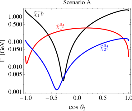
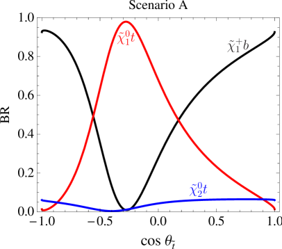
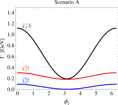
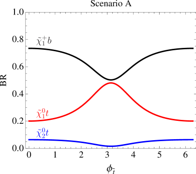
Figure 1: Decay widths (left column) and branching ratios (right column) for $\tilde{t}_{1}$ in Scenario A as a function of the stop mixing angle $\cos\theta_{\tilde{t}}$ (upper row) and the stop CP phase $\phi_{\tilde{t}}$ (lower row). Black, red and blue lines are for the $\tilde{\chi}^{+}_{1}b$, $\tilde{\chi}^{0}_{1}\,t$ and $\tilde{\chi}^{0}_{2}\,t$ final states, respectively.

Although Scenario A does not contain CP phases, we include them here to analyze the sensitivity of the decay widths and the branching ratios. The respective plots can be seen in the lower row of Fig. 1. The most significant change is for the decay to a chargino and a bottom quark. This results from the third term of Eq. (52) that changes sign when varying $\phi_{\tilde{t}}$ from 0 to $\pi$ giving destructive interference. Although the dependence on $\phi_{\tilde{t}}$ is clearly visible the constraints on this parameter, as we will see it later, will be rather weak.

Scenario B – mixed gaugino/higgsino $\tilde{\chi}_{1}^{+}$ and $\tilde{\chi}^{0}_{2}$

The situation changes significantly in Scenario B. The second chargino $\tilde{\chi}^{+}_{2}$ is now lighter than the stop $\tilde{t}_{1}$ so there is a new decay channel open. Both charginos and the neutralino $\tilde{\chi}^{0}_{2}$ now have a significant higgsino component. The dependence on the stop mixing angle of all the decay widths is much flatter now, as can be seen in the left panel of Fig. 2. We note a well pronounced enhancement of the decay widths for right stops (around $\cos\theta_{\tilde{t}}=0$). For charginos it can be understood by looking at Eq. (45) where the coupling of $\tilde{t}_{R}$ is proportional to the large top Yukawa coupling, whereas the coupling of $\tilde{t}_{L}$ is proportional to the smaller bottom Yukawa coupling. For the decay to $\tilde{\chi}^{0}_{2}\,t$ the enhancement is due to the left-right interference term, whereas for $\tilde{\chi}^{0}_{1}\,t$ it is due to the quadratic term in Eq. (54).

Thanks to the presence of the higgsino component in charginos and neutralinos, we now become more sensitive to the phase $\phi_{\tilde{t}}$, see the right panel of Fig. 2. Apart from the decay to $\tilde{\chi}^{0}_{2}\,t$, all other decay widths can change by up to an order of magnitude depending on the CP phase. The former remains almost unchanged due to the accidental cancellations between two terms of Eq. (54). For the decays to charginos $\tilde{\chi}_{1}^{\pm}$ ($\tilde{\chi}_{2}^{\pm}$) the suppression (enhancement) of the decay width with the phase arises due to change of the sign of $\cos\phi_{\tilde{t}}$ when $\phi_{\tilde{t}}\to\pi$, cf. Eqs. (52) and (53). The difference for $\tilde{\chi}_{1}^{+}$ and $\tilde{\chi}_{2}^{+}$ is the result of the sign difference between $V_{11}V_{12}^{*}$ and $V_{21}V_{22}^{*}$.

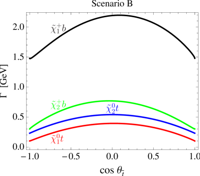
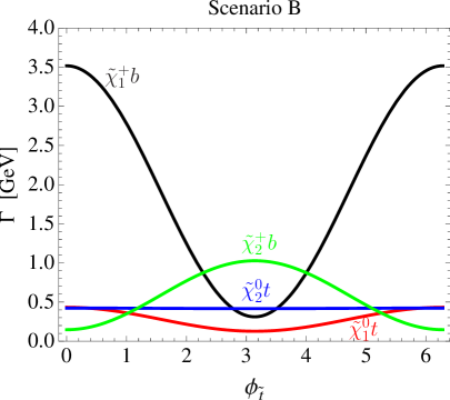
Figure 2: Decay widths for $\tilde{t}_{1}$ in Scenario B as a function of the stop mixing angle $\cos\theta_{\tilde{t}}$ (left panel) and the stop CP phase $\phi_{\tilde{t}}$ (right panel). Black, red, blue and green lines are for the $\tilde{\chi}^{+}_{1}b$, $\tilde{\chi}^{0}_{1}\,t$, $\tilde{\chi}^{0}_{2}\,t$ and $\tilde{\chi}^{+}_{2}b$ final states, respectively.

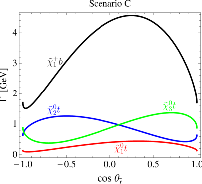
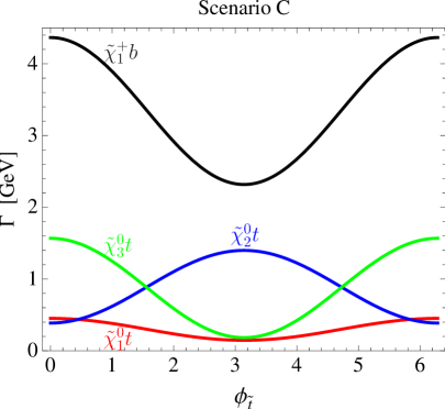
Figure 3: Decay widths for $\tilde{t}_{1}$ in Scenario C as a function of the stop mixing angle $\cos\theta_{\tilde{t}}$ (left panel) and the stop CP phase $\phi_{\tilde{t}}$ (right panel). Black, red, blue and green lines are for the $\tilde{\chi}^{+}_{1}b$, $\tilde{\chi}^{0}_{1}\,t$, $\tilde{\chi}^{0}_{2}\,t$ and $\tilde{\chi}^{0}_{3}\,t$ final states, respectively.

Scenario C – higgsino-like $\tilde{\chi}_{1}^{+}$, $\tilde{\chi}^{0}_{2}$ and $\tilde{\chi}^{0}_{3}$

The last discussed scenario features the hierarchy $M_{1}<\mu<M_{2}$. Therefore the light chargino and neutralinos $\tilde{\chi}^{0}_{2}$, $\tilde{\chi}^{0}_{3}$ are higgsino-like with small mass differences between them. The lightest neutralino is bino-like as in the previous scenarios. The dependence of the decay widths on the stop mixing angle has been shown in the left panel of Fig. 3. The difference in the decay widths to the chargino for left and right stops is a consequence of the $Y_{t}$ coupling for right states in Eq. (45). A similar effect was seen in Scenario B, however it is now more pronounced due to the higgsino nature of the light chargino $\tilde{\chi}_{1}^{+}$. We also observe the interesting exchange of the decay widths to heavier neutralinos when the sign of $\cos\theta_{\tilde{t}}$ changes. This feature arises due to the $Y_{t}^{2}\>{\rm Re}\left[N_{j4}^{*2}\right]$ term in the second line of Eq. (56) that is enhanced both by the large top Yukawa coupling and the higgsino nature of the two neutralinos. Since neutralinos $\tilde{\chi}^{0}_{2}$ and $\tilde{\chi}^{0}_{3}$ have opposite intrinsic CP parities in Scenario C, cf. Ref. [44], the entries in the neutralino mixing matrix that correspond to $\tilde{\chi}^{0}_{3}$ are purely imaginary. Therefore, the contribution has an opposite sign in the decay width and hence different behaviour with respect to the sign of $\cos\theta_{\tilde{t}}$.

A similar dependence of the decay widths $\tilde{\chi}^{0}_{2}\,t$ and $\tilde{\chi}^{0}_{3}\,t$ on the sign of $\cos\phi_{\tilde{t}}$ can be seen in the right panel of Fig. 3. Its origin is the same as in the above discussed case for $\cos\theta_{\tilde{t}}$. As before the change in the width of the decay to $\tilde{\chi}^{+}_{1}b$ is caused by a change in the sign of the last term of Eq. (52) with $\cos\phi_{\tilde{t}}$, as $\phi_{\tilde{t}}$ is varied from 0 to $\pi$. It is interesting to note that now the width for the decay to chargino $\tilde{\chi}_{1}^{+}$ does not show as strong dependence on the phase $\phi_{\tilde{t}}$ compared to Scenario B. However, the dependence of the branching ratios for the decays to neutralinos is still well pronounced.

4 Potential observables at the LHC

4.1 Ratios of branching ratios

As one can see in Figs. 1, 2 and 3, the decay widths can change by up to a few orders of magnitude depending on the stop mixing angle and the CP phase. In addition, the branching ratios are also very sensitive to these parameters. However, since the measurement of decay widths and branching ratios will be difficult at the LHC we propose to analyze the ratios of branching ratios. That means comparing the number of stops decaying to one final state with the number of stops decaying to another final state. Having three decay modes possible we can define the following ratios of branching ratios for each of the Scenarios A, B and C:

$$R_{1t}^{1b}=\frac{BR(\tilde{t}_{1}\to\tilde{\chi}^{+}_{1}b)}{BR(\tilde{t}_{1}\to\tilde{\chi}^{0}_{1}\,t)},\qquad R_{2t}^{1b}=\frac{BR(\tilde{t}_{1}\to\tilde{\chi}^{+}_{1}b)}{BR(\tilde{t}_{1}\to\tilde{\chi}^{0}_{2}\,t)},\qquad R_{2t}^{1t}=\frac{BR(\tilde{t}_{1}\to\tilde{\chi}^{0}_{1}\,t)}{BR(\tilde{t}_{1}\to\tilde{\chi}^{0}_{2}\,t)}\,.$$ (57)

Figure 4 shows the above ratios of branching ratios in Scenario A as functions of $\cos\theta_{\tilde{t}}$ and the CP-violating phase $\phi_{\tilde{t}}$. For Scenario B we have three additional combinations due to the decay $\tilde{t}_{1}\to\tilde{\chi}^{+}_{2}b$ being open,

$$R_{2b}^{1b}=\frac{BR(\tilde{t}_{1}\to\tilde{\chi}^{+}_{1}b)}{BR(\tilde{t}_{1}\to\tilde{\chi}^{+}_{2}b)},\qquad R_{2b}^{1t}=\frac{BR(\tilde{t}_{1}\to\tilde{\chi}^{0}_{1}\,t)}{BR(\tilde{t}_{1}\to\tilde{\chi}^{+}_{2}b)},\qquad R_{2b}^{2t}=\frac{BR(\tilde{t}_{1}\to\tilde{\chi}^{0}_{2}\,t)}{BR(\tilde{t}_{1}\to\tilde{\chi}^{+}_{2}b)}\,.$$ (58)

For Scenario C due to the decay $\tilde{t}_{1}\to\tilde{\chi}^{0}_{3}\,t$ being allowed we have

$$R_{3t}^{1b}=\frac{BR(\tilde{t}_{1}\to\tilde{\chi}^{+}_{1}b)}{BR(\tilde{t}_{1}\to\tilde{\chi}^{0}_{3}\,t)},\qquad R_{3t}^{1t}=\frac{BR(\tilde{t}_{1}\to\tilde{\chi}^{0}_{1}t)}{BR(\tilde{t}_{1}\to\tilde{\chi}^{0}_{3}\,t)},\qquad R_{3t}^{2t}=\frac{BR(\tilde{t}_{1}\to\tilde{\chi}^{0}_{2}\,t)}{BR(\tilde{t}_{1}\to\tilde{\chi}^{0}_{3}\,t)}\,.$$ (59)

Because of the higgsino nature of neutralinos $\tilde{\chi}^{0}_{2}$ and $\tilde{\chi}^{0}_{3}$ they are very close in mass and it might turn out that they are impossible to disentangle at the LHC. Therefore we define two additional ratios by combining the decay modes to $\tilde{\chi}^{0}_{2}\,t$ and $\tilde{\chi}^{0}_{3}\,t$

$$R_{23t}^{1b}=\frac{BR(\tilde{t}_{1}\to\tilde{\chi}^{+}_{1}b)}{BR(\tilde{t}_{1}\to\tilde{\chi}^{0}_{2}\,t)+BR(\tilde{t}_{1}\to\tilde{\chi}^{0}_{3}\,t)}\>,\qquad R_{23t}^{1t}=\frac{BR(\tilde{t}_{1}\to\tilde{\chi}^{0}_{1}t)}{BR(\tilde{t}_{1}\to\tilde{\chi}^{0}_{2}\,t)+BR(\tilde{t}_{1}\to\tilde{\chi}^{0}_{3}\,t)}\,.$$ (60)

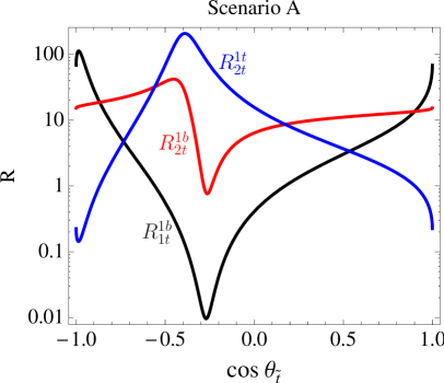
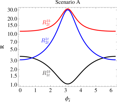
Figure 4: Ratios of branching ratios as a function of stop mixing angle $\cos\theta_{\tilde{t}}$ and CP phase $\phi_{\tilde{t}}$ in Scenario A, left and right panel, respectively. Black, red and blue lines are for the ratios ${R}_{1t}^{1b}$, ${R}_{2t}^{1b}$ and ${R}_{2t}^{1t}$ (see Eq. (57)), respectively.

In our analysis we focus on direct stop production $pp\to\tilde{t}_{1}\tilde{t}_{1}^{*}$ in order to have better control on the number of observed stops and to reduce the background due to bottom squarks. In the SPS1a^′ scenario the cross section for this process amounts to 3.44 pb at the next-to-leading order [18, 43], whereas the total SUSY cross section is 60 pb. Due to mass splitting between stop states the cross section for $pp\to\tilde{t}_{2}\tilde{t}^{*}_{2}$ is much smaller with a value of 0.26 pb. Similarly for sbottoms we get $\sigma(pp\to\tilde{b}_{1}\tilde{b}_{1}^{*})=0.6$ pb and $\sigma(pp\to\tilde{b}_{2}\tilde{b}_{2}^{*})=0.4$ pb. This gives a relatively clean environment for the observation of direct light stop pair production and further reduction after cuts may be expected. Possible final states are as follows:

$$pp\to\tilde{t}_{1}\tilde{t}_{1}^{*}\to t\tilde{\chi}^{0}_{2}+\bar{t}\tilde{\chi}^{0}_{2}\to t\ell^{+}{\ell^{-}}\tilde{\chi}^{0}_{1}+\bar{t}\ell^{+}{\ell}^{-}\tilde{\chi}^{0}_{1}\to 4\ell\>4j\>2b\ +E_{\rm miss}\,,$$ (61)

$$pp\to\tilde{t}_{1}\tilde{t}_{1}^{*}\to t\tilde{\chi}^{0}_{2}+\bar{t}\tilde{\chi}^{0}_{1}\to t\ell^{+}{\ell}^{-}\tilde{\chi}^{0}_{1}+\bar{t}\tilde{\chi}^{0}_{1}\to 2\ell\>4j\>2b+E_{\rm miss}\,,$$ (62)

$$pp\to\tilde{t}_{1}\tilde{t}_{1}^{*}\to t\tilde{\chi}^{0}_{2}+b\tilde{\chi}^{+}_{1}\to t\ell^{+}{\ell}^{-}\tilde{\chi}^{0}_{1}+b{\ell}^{+}\nu_{\ell}\tilde{\chi}^{0}_{1}\to 3\ell\>2j\>2b+E_{\rm miss}\,,$$ (63)

$$pp\to\tilde{t}_{1}\tilde{t}_{1}^{*}\to t\tilde{\chi}^{0}_{1}+\bar{t}\tilde{\chi}^{0}_{1}\to 4j\>2b+E_{\rm miss}\,,$$ (64)

$$pp\to\tilde{t}_{1}\tilde{t}_{1}^{*}\to t\tilde{\chi}^{0}_{1}+b\tilde{\chi}^{+}_{1}\to t\tilde{\chi}^{0}_{1}+b{\ell}^{+}\nu_{\ell}\tilde{\chi}^{0}_{1}\to\ell\>2j\>2b\>+E_{\rm miss}\,,$$ (65)

$$pp\to\tilde{t}_{1}\tilde{t}_{1}^{*}\to\bar{b}\tilde{\chi}^{-}_{1}+b\tilde{\chi}^{+}_{1}\to\bar{b}\ell^{-}\bar{\nu}_{\ell}\tilde{\chi}^{0}_{1}+b{\ell}^{+}\nu_{\ell}\tilde{\chi}^{0}_{1}\to 2\ell\>2b\>+E_{\rm miss}\,.$$ (66)

The production process itself can be tagged using a clean decay mode for one of the stops, for instance the decay to $\tilde{\chi}^{0}_{2}\,t$ followed by a leptonic neutralino decay and hadronic top decay. For an integrated luminosity of $\mathcal{L}=100\;\mathrm{fb}^{-1}$ we would have more than $300\,000$ stop pair production events in the case of SPS1a^′ scenario. Assuming that on average $10\%$ of charginos and neutralinos decay to leptons [42], taking into account the hadronic top branching ratio and varying a selection efficiency of $1\%$, $3\%$ and $5\%$, one can expect roughly 350, 1000 and 1750 events to be observed, respectively. A further increase in the integrated luminosity will result in larger samples. Therefore in our further analysis we will study the case when 1000 events have been correctly identified and show that with this amount of experimental data one can still get strong constraints on the stop mixing angle and the mass.

The other important point we wish to emphasize are the branching ratios for decays of the chargino $\tilde{\chi}^{\pm}_{1}$ and the neutralino $\tilde{\chi}^{0}_{2}$ into leptons. Although one may expect that the related uncertainty will cancel out to some extent in the ratio $R^{1b}_{2t}$ (as in our scenarios $\tilde{\chi}^{\pm}_{1}$ and $\tilde{\chi}^{0}_{2}$ have similar gaugino/higgsino composition), this is not true for the other ratios involving decays to the LSP. Since our focus here is on the stop sector we assume that the leptonic branching ratios of the charginos and neutralinos are known. However, as this would require a better knowledge of the gaugino/higgsino structure, it is possible that the measurements from the LHC would have to be supplemented by the linear collider experiment. Here charginos and neutralinos can be measured with a high precision $\mathcal{O}(1\%)$, see Ref. [38] and references therein. This would be an interesting example of LHC/ILC interplay [19], in particular for the scenarios where direct stop production is beyond the kinematical reach of the ILC.

A large number of SUSY and SM backgrounds are expected for stop production at the LHC. The most severe Standard Model background, especially for the channels Eqs. (64)–(66), will be $t\bar{t}$ production. The issue of whether these signals can be distinguished from the background is under discussion and requires further experimental studies. For instance, the analysis in Ref. [22] shows that within certain region of stop masses discovery looks promising in the $t\bar{t}+E_{\mathrm{miss}}$ channel with fully hadronic top decays. A more recent study [35], using the top-tagging [37] technique showed that the SM $t\bar{t}$ background can be manageable for the final state Eq. (64).

The most important SUSY background process is going to be gluino production with subsequent decays to stops or sbottoms. One important difference between the signal and these backgrounds is the number of $b$-jets. The signal event always results in exactly 2 $b$-jets, whereas SUSY backgrounds will typically have 4 $b$-jets and this feature can be used to suppress them. On the other hand, squark production followed by decay to chargino and leptonic chargino decay will also result in 2 jets and 2 leptons in the final state with a rather high rate. This can fake the signal process Eq. (66). However, the background will have two light quark jets instead of $b$-jets. Therefore, in order to extract the signal, good $b$-jet tagging efficiency and light jet rejection will be needed [4]. Requiring at least one and no more than two $b$-jets to be tagged would suppress the backgrounds significantly.

Another method of getting a handle on the supersymmetric and the Standard Model backgrounds has been discussed in [36]. Using kinematic reconstruction, it was shown that for the final states containing $\tilde{\chi}^{0}_{2}\to\ell^{+}\ell^{-}\tilde{\chi}^{0}_{1}$ one can suppress the SUSY backgrounds to the signal level and, at the same time, practically remove the SM contributions. This method gave a $S/B$ ratio of order 1, with an efficiency of about 5% depending upon the scenario. This is an encouraging result and the application to other final states, Eqs. (61)–(66), will be investigated.

Finally, we note that the signal process with leptonic top decay, e.g. $\tilde{\chi}^{0}_{1}\,t\to b\ell+E_{\rm miss}$, can give the same final state as the decay mode with charginos, i.e. $\tilde{\chi}^{+}_{1}b\to b\ell+E_{\rm miss}$. However, we note that this complication does not affect the result of the fit since it does not introduce any new unknown parameters. The fitted observables would be a linear combination of the original ones, Eq. (57), and the fit would rely on the same set of information. Hence, one can combine the above channels and actually enhance the signal.

An important note is that it will not be sufficient to simply remove as much background as possible using the relevant cuts. We will also need to understand with a high degree of accuracy how each individual signal channel will be affected by the backgrounds. Understanding the background well is required, as for each channel we study, the number of background events contaminating the sample will be different. Therefore the pollution due to backgrounds will affect our ratios of branching ratios. The reconstruction efficiency, cuts and triggers will also have a different effect on each channel and will have to be well understood for our measurements to be accurate. Another complication will be higher-order QCD effects, in particular in case of hadronic top decays. However, the study of this type will require high integrated luminosity and after a long running time these issues should be much better understood. We leave a detailed analysis of these effects for our different final states and the additional uncertainties for future work.

To summarize, a successful application of the method presented here will require a good understanding of the detectors and backgrounds. This may become possible after a few years of the LHC operating in the high luminosity mode. Also, new analysis techniques that are being constantly developed should improve our control of the backgrounds. In line with the results presented in [35, 36] we therefore assume that a signal-to-background ratio close to 1 can be achieved. This will lead to the increased error on the measured number of events by a factor $\sqrt{3}$. In the following, we take the slightly more conservative assumption that the error is twice that of the statistical error alone. A more reliable estimate will require a complete simulation of signal and background processes.

4.2 Determination of stop mass and mixing angle

In order to show the possible advantages of using ratios of branching ratios for the analysis of the stop sector we first define the normalized ratios

$$\widehat{R}_{j}^{i}=R_{j}^{i}-R^{i\>\mathrm{nominal}}_{j}\quad\mbox{with}\quad R^{i\>\mathrm{nominal}}_{j}=R_{j}^{i}(\cos\theta^{\mathrm{nominal}}_{\tilde{t}})\,,$$ (67)

where $\theta^{\mathrm{nominal}}_{\tilde{t}}$ is the actual mixing angle in the given scenario and $i$, $j$ run over all possible channels, i.e. $1b$, $1t$, $2t$ etc., cf. Eqs. (57)–(60). According to this definition $\widehat{R}_{i}(\cos\theta^{\mathrm{nominal}}_{\tilde{t}})\equiv 0$. Furthermore, we assume that we have $n=1000$ of well identified events of stop $\tilde{t}_{1}\tilde{t}_{1}^{*}$ pair production. We now take the expected number of events in each decay mode $n_{i}=n\times BR_{i}$. Note that $1=\sum n_{i}$ only if decays to charginos and neutralinos are the only possible decay channels. One should be aware that for our method it is not necessary to measure all possible decay modes, as explained later. The statistical error for $n_{i}$ is $(\Delta n_{i})_{\mathrm{stat}}=\sqrt{n_{i}}$. In order to account for some of the expected additional uncertainties, e.g. due to background subtraction, in the following $\chi^{2}$ fits we decide to use twice as large error, i.e.

$$\Delta n_{i}=2(\Delta n_{i})_{\mathrm{stat}}=2\sqrt{n_{i}}\;.$$ (68)

The resulting error for ratios of branching ratios is given by

$$\Delta R_{j}^{i}=\sqrt{\left(\frac{\Delta n_{i}}{n_{j}}\right)^{2}+\left(\frac{n_{i}\Delta n_{j}}{n_{j}^{2}}\right)^{2}}\qquad\mathrm{with}\qquad R_{j}^{i}=\frac{n_{i}}{n_{j}}\>.$$ (69)

Before analyzing the expected accuracy of determination of stop sector parameters let us study the possible influence of the gaugino/higgsino sector parameters, taking as an example Scenario A. The precise knowledge of the LSP mass and the mixing angles of the charginos and the neutralinos may only be accessible after the results from a linear $e^{+}e^{-}$ collider are available. In Fig. 5 we show the dependence of the normalized ratios Eq. (57) on the gaugino mass parameter $M_{2}$ and the mass of the LSP, $m_{\mathrm{LSP}}\equiv m_{\tilde{\chi}^{0}_{1}}$. In the left plot of Fig. 5 we keep the mass differences $m_{\tilde{\chi}^{0}_{2}}-m_{\tilde{\chi}^{0}_{1}}$ and $m_{\tilde{\chi}^{\pm}_{1}}-m_{\tilde{\chi}^{0}_{1}}$ fixed as these are expected to be measured with high precision at the LHC. As can be seen, the value of $\widehat{R}_{1t}^{1b}$ is very stable in both cases, whilst $\widehat{R}_{2t}^{1b}$ and $\widehat{R}_{2t}^{1t}$ exhibit an increase for larger values of $M_{2}$ and $m_{\mathrm{LSP}}$. This is because both $\widehat{R}_{2t}^{1b}$ and $\widehat{R}_{2t}^{1t}$ include a branching ratio for the decay to $\tilde{\chi}^{0}_{2}\,t$ that is close to its kinematic threshold. Therefore, for an increasing $m_{\mathrm{LSP}}$ or $M_{2}$ (note that $M_{1}\simeq m_{\tilde{\chi}^{0}_{1}}$ and $M_{2}\simeq m_{\tilde{\chi}^{0}_{2}}$ in Scenario A) we approach the point where this decay becomes impossible. High sensitivity of the decay width near the threshold means that to use such a decay mode to determine the mixing angle, one would have to know the masses extremely precisely. In this case the ratio of branching ratios is no longer a good observable. Moreover the branching ratio for such a decay usually becomes very small.

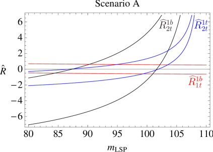
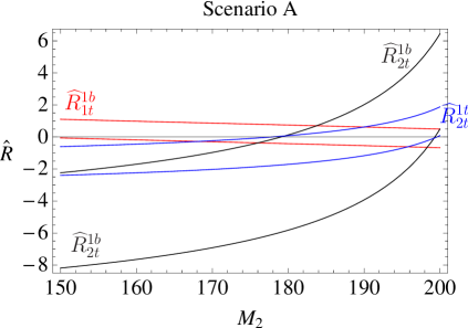
Figure 5: Dependence of the normalized ratios of branching ratios $\widehat{R}_{i}$, Eq. (67), in stop decays on the mass of the lightest neutralino (left panel) and the gaugino mass parameter $M_{2}$ (right panel) in Scenario A. The values of the other parameters and the mass difference between the LSP and $\tilde{\chi}^{0}_{2}$, $\tilde{\chi}_{1}^{\pm}$ for the left plot are fixed to their nominal values. Red lines are for $\widehat{R}_{1t}^{1b}$, black lines for $\widehat{R}_{2t}^{1b}$, and blue lines for $\widehat{R}_{2t}^{1t}$, see Eq. (57). The upper and lower lines show the band due to 1-$\sigma$ uncertainty with respect to the central value as defined in Eq. (69).

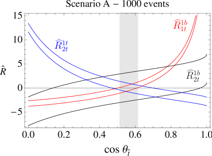
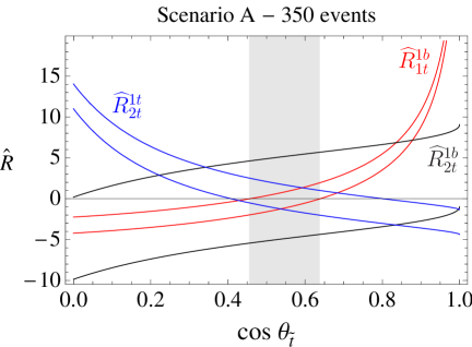
Figure 6: Normalized ratios $\widehat{R}_{j}^{i}$, Eq. (67), near the nominal value of $\cos\theta_{\tilde{t}}=0.56$ for Scenario A. Red lines are for $\widehat{R}_{1t}^{1b}$, black lines for $\widehat{R}_{2t}^{1b}$, and blue lines for $\widehat{R}_{2t}^{1t}$, see Eq. (57). The upper and lower lines show the 1-$\sigma$ uncertainty as defined in the text. The region allowed by all three ratios is shaded in grey. Left panel is for 1000 identified events, right panel for 350 events.

In order to analyze the possible accuracy in extracting the mixing parameters of the stop sector we start with the example of Scenario A. In Fig. 6 we show the behaviour of the normalized ratios of branching ratios, Eq. (67), near the nominal value of the mixing angle $\cos\theta^{\mathrm{nominal}}_{\tilde{t}}$ for 1000 and 350 events, left and right panel, respectively. Using only one of three possible ratios, the smallest error and hence the best estimate we get is using the ratio $\widehat{R}_{1t}^{1b}$, which depends on the dominant decay modes $\tilde{\chi}^{0}_{1}\,t$ and $\tilde{\chi}^{+}_{1}b$. For the ratio $\widehat{R}_{2t}^{1t}$ the impact of the error is slightly larger due to the limited statistics. On the other hand the ratio $\widehat{R}_{2t}^{1b}$ gives the weakest constraints because both $\tilde{\chi}^{+}_{1}$ and $\tilde{\chi}^{0}_{2}$ are winos, hence their couplings to $\tilde{t}_{1}$ follow a similar pattern. We assume here that the values of the other SUSY parameters, including the $\tilde{t}_{1}$ mass, are known. Using only the information from the ratio $\widehat{R}_{1t}^{1b}$ we get the estimate

$$0.51<\cos\theta_{\tilde{t}}<0.62$$ (70)

at the 1-$\sigma$ level, see Fig. 6, with 1000 events. We also show the plots when only 350 events are included. In this case, we can expect the following sensitivity

$$0.45<\cos\theta_{\tilde{t}}<0.64\;,$$ (71)

with the allowed range increased by a factor $\sim 2$.

Having at hand three possible decay modes we can constrain not only the mixing angle $\cos\theta_{\tilde{t}}$ but also the mass of the light stop quark and the CP-violating phase $\phi_{\tilde{t}}$. We use a $\chi^{2}$ fit defined as follows:

$$\chi^{2}=\sum_{\{i,j\}}\left(\frac{R_{j}^{i}(\cos\theta_{\tilde{t}})-R_{j}^{i\>\mathrm{nominal}}}{\Delta R_{j}^{i}}\right)^{2}\,,$$ (72)

where the error is defined by Eq. (69) and the sum runs over the respective ratios for each of the scenarios, e.g. $\{i,j\}=\{\{1b,1t\},\{1b,2t\},\{1t,2t\}\}$ in Scenario A, cf. Eqs (57)–(60). The results of fitting the stop mass $m_{\tilde{t}_{1}}$ and the mixing angle $\cos\theta_{\tilde{t}}$ in Scenario A are shown in the left panel of Fig. 7. We find two minima of $\chi^{2}$ that fit the input data well. In order to resolve the two-fold ambiguity, additional observables will be needed. Assuming that we can pin down the correct solution we get the following 1-$\sigma$ (2-$\sigma$) estimate of the two parameters

$$m_{\tilde{t}_{1}}=366^{+6\;(+18)}_{-3\;(-5)}\,,\qquad\cos\theta_{\tilde{t}}=0.56\pm 0.05\;(\pm 0.1)\,,\qquad\theta_{\tilde{t}}=0.98^{+0.06\;(+0.11)}_{-0.06\;(-0.13)}$$ (73)

for 1000 events assuming the errors defined in Eqs. (68) and (69) and neglecting other uncertainties. The mixing angle obtained here should be treated as an effective parameter, as discussed in Sec. 3.1. The better lower bound for the measured mass is a consequence of reaching the kinematic threshold for the decay ${\tilde{t}_{1}}\to\tilde{\chi}^{0}_{2}t$. In the right panel of Fig. 7 we show the results of the $\chi^{2}$ fit to the mixing angle and the phase $\phi_{\tilde{t}}$. As expected, the sensitivity to the CP phase is poor and taking into account the possible ambiguity in the mixing angle $\cos\theta_{\tilde{t}}$, the full range of phases remains allowed. The same set of plots in the case of 350 identified events is shown in Fig. 8, giving

$$m_{\tilde{t}_{1}}=366^{+14\;(+80)}_{-3\;(-7)}\,,\qquad\cos\theta_{\tilde{t}}=0.56\pm 0.08\;(\pm 0.15)\,,\qquad\theta_{\tilde{t}}=0.98^{+0.10\;(+0.17)}_{-0.10\;(-0.20)}\;,$$ (74)

at the 1-$\sigma$ (2-$\sigma$) level, respectively.

Figure 7: A $\chi^{2}$ fit of ratios ${R}_{1t}^{1b}$, ${R}_{2t}^{1b}$ and ${R}_{2t}^{1t}$, Eq. (57), to the stop mass and the mixing angle $\cos\theta_{\tilde{t}}$ (left panel), and the stop mixing angle and the CP phase $\phi_{\tilde{t}}$ (right panel) in Scenario A for $n=1000$ events. Bold, normal and dashed lines are for 1-, 2- and 3-$\sigma$ contours, respectively.

Figure 8: Same as Fig. 7, Scenario A, but for 350 identified stop decays.

The situation changes for Scenarios B and C. We now have 6 possible ratios in each case, for Scenario B: ${R}_{1t}^{1b}$, ${R}_{2t}^{1b}$, ${R}_{2t}^{1t}$, ${R}_{2b}^{1b}$, ${R}_{2b}^{1t}$, ${R}_{2b}^{2t}$, and for Scenario C: ${R}_{1t}^{1b}$, ${R}_{2t}^{1b}$, ${R}_{2t}^{1t}$, ${R}_{3t}^{1b}$, ${R}_{3t}^{1t}$, ${R}_{3t}^{2t}$. The results of the fit in Scenario B have been shown in Figs. 9 and 10 for 1000 and 350 events, respectively. Corresponding plots for Scenario C are presented in Figs. 11 and 12. We again consider two cases: fitting of the mass $m_{\tilde{t}}$ together with the mixing angle $\cos\theta_{\tilde{t}}$ and fitting of the mixing angle together with the CP-violating phase. In both cases we assume that the value of the third parameter is known. Charginos and neutralinos now have a significant higgsino component and, as we saw in Figs. 2 and 3, the dependence on the mixing angle is much weaker. Therefore the constraints for the mixing angle and the mass that we get are not as good as in the case of Scenario A. It is interesting to note that in general the results of the fit are better in Scenarios A and C (gaugino and higgsino, respectively) than in Scenario B (mixed case). Consequently we conclude that the scenario with strong mixing between gauginos and higgsinos would be the most difficult to resolve. This is visible for the 350-event case in Scenario B (Fig. 10), where the mixing angle and the phase are practically unconstrained.

Figure 9: A $\chi^{2}$ fit of ratios ${R}_{1t}^{1b}$, ${R}_{2t}^{1b}$, ${R}_{2t}^{1t}$, ${R}_{2b}^{1b}$, ${R}_{2b}^{1t}$ and ${R}_{2b}^{2t}$, Eq. (57) and Eq. (58), to the stop mass and the mixing angle $\cos\theta_{\tilde{t}}$ (left panel), and the stop mixing angle and the CP phase $\phi_{\tilde{t}}$ (right panel) in Scenario B for $n=1000$ events. Bold, normal and dashed lines are for 1-, 2- and 3-$\sigma$ contours, respectively.

Figure 10: Same as Fig. 9, Scenario B, but for 350 identified stop decays.

Analyzing both the mixing angle and the phase, we obtain four allowed regions. Nevertheless smaller regions are allowed for the CP phase as our observables are more sensitive to it than in Scenario A. Branching ratios are CP-even observables, therefore they cannot resolve ambiguities for the CP phase. This shows that for precise measurements in the stop sector one has to use CP-odd observables, like triple products of momenta [36, 41, 45]. Only such a combined analysis of CP-even and CP-odd observables can give an unambiguous determination of the stop sector parameters.

Figure 11: A $\chi^{2}$ fit of ratios ${R}_{1t}^{1b}$, ${R}_{2t}^{1b}$, ${R}_{2t}^{1t}$, ${R}_{3t}^{1b}$, ${R}_{3t}^{1t}$ and ${R}_{3t}^{2t}$, Eq. (57) and Eq. (59), to the stop mass and the mixing angle $\cos\theta_{\tilde{t}}$ (left panel) and the stop mixing angle and the CP phase $\phi_{\tilde{t}}$ (right panel) in Scenario C for $n=1000$ events. Bold, normal and dashed lines are for 1-, 2- and 3-$\sigma$ contours, respectively.

Figure 12: Same as Fig. 11, Scenario C, but for 350 identified stop decays.

Finally, we note that in Scenario C it might be difficult to resolve the decays $\tilde{\chi}^{0}_{2}\,t$ and $\tilde{\chi}^{0}_{3}\,t$, as the two close-in-mass higgsino-like neutralinos may be difficult to disentangle at the LHC. After combining decay modes of the two neutralinos we lose much of the sensitivity to the elements of the stop mixing matrix. In such cases, precise measurements in the neutralino and chargino sectors will be essential. The measurements of the masses and couplings of these particles may be possible with high accuracy at the linear collider.

5 Conclusions

As stops play an important role in the MSSM, it is crucial to measure their couplings and masses at future colliders in order to understand the underlying model. Therefore we have proposed a promising way to get hints of the stop sector parameters at the LHC by studying the dependence of branching ratios in various mixing scenarios. In particular, we have discussed the couplings and the decays of the supersymmetric top partners to the charginos and the neutralinos.

A careful analysis of the couplings of scalar tops to electroweak gauginos and higgsinos shows a strong dependence on the mixing angle and the CP-violating phase of the stop sector. This effect arises due to the structure of the electroweak gauge couplings and the Yukawa couplings of left and right stop states. We have analyzed three benchmark scenarios with different structures for the gaugino and higgsino sectors, where the light charginos and neutralinos had gaugino-like, higgsino-like or mixed composition. Analysis of the decay widths and the branching ratios has shown a strong relation between the stop mixing parameters and the decay pattern in each of the scenarios.

Next, we have discussed a possible approach to get a handle on the light stop mass, the mixing angle $\theta_{\tilde{t}}$ and the CP-violating phase $\phi_{\tilde{t}}$ at the Large Hadron Collider. Since stops will be produced in large numbers at this machine one can hope to learn the stop properties from their decay pattern. As the branching ratios are going to be difficult to be measured at the LHC, we propose to analyze the ratios of branching ratios for different decay modes. These observables inherit a strong dependence on the mixing angle from stop decay widths and therefore can be a sensitive probe of the stop sector. Since they rely only on the relative numbers of stops decaying via various channels, many experimental uncertainties will cancel. In particular, one does not need to control all of the possible decay modes. In fact, as we have shown for the SPS1a^′ parameter point, using only two decay modes can give good constraints on the stop mixing angle. Finally we have performed $\chi^{2}$ fits to show that the ratios of branching ratios can give strong bounds on the parameters of the stop sector: the mass of $\tilde{t}_{1}$, the stop mixing angle $\cos\theta_{\tilde{t}}$ and the CP-violating phase $\phi_{\tilde{t}}$. The expected accuracy depends upon the scenario studied but looks the most promising for mSUGRA models.

In the present study many of the experimental uncertainties have been neglected. Backgrounds have not been explicitly included, but assuming that they can be successfully controlled, as discussed, we extrapolated their possible impact by doubling the usual statistical error. It is clear that more detailed experimental studies are needed to assess the feasibility of the method in the harsh LHC environment and its possible accuracy. However, taking into account the importance of the stop sector for our understanding of the supersymmetric model, we think that such a study deserves further attention. Application of this method will require the study of many possible final states to understand those that are most promising. In addition a good control of detector effects, like fake rates for leptons and $b$-jets, and SM as well as SUSY backgrounds will be needed, but these are not yet included. These uncertainties will certainly lead to the method presented here having lower sensitivity. However, we believe that the results obtained here, even with a rather low number of events, are encouraging enough to pursue further studies of precision measurements in the stop sector.

References

- [1] Yu. A. Golfand and E. P. Likhtman, JETP Lett. 13 (1971) 323 [Pisma Zh. Eksp. Teor. Fiz. 13 (1971) 452]; D. V. Volkov and V. P. Akulov, Phys. Lett. B 46 (1973) 109; J. Wess and B. Zumino, Phys. Lett. B 49 (1974) 52; Nucl. Phys. B 70 (1974) 39; for reviews see e.g. H. P. Nilles, Phys. Rept. 110 (1984) 1; H. E. Haber and G. L. Kane, Phys. Rept. 117 (1985) 75; D. J. H. Chung, L. L. Everett, G. L. Kane, S. F. King, J. D. Lykken and L. T. Wang, Phys. Rept. 407 (2005) 1 [arXiv:hep-ph/0312378].
- [2] J. R. Ellis, S. Heinemeyer, K. A. Olive, A. M. Weber and G. Weiglein, JHEP 0708 (2007) 083 [arXiv:0706.0652 [hep-ph]]; O. Buchmueller et al., JHEP 0809 (2008) 117 [arXiv:0808.4128 [hep-ph]].
- [3] G. L. Bayatian et al. [CMS Collaboration], J. Phys. G 34 (2007) 995.
- [4] G. Aad et al. [The ATLAS Collaboration], arXiv:0901.0512 [hep-ex].
- [5] I. Hinchliffe, F. E. Paige, M. D. Shapiro, J. Soderqvist and W. Yao, Phys. Rev. D 55 (1997) 5520 [arXiv:hep-ph/9610544].
- [6] J. A. Aguilar-Saavedra et al., Eur. Phys. J. C 46 (2006) 43 [arXiv:hep-ph/0511344].
- [7] J. Hisano, K. Kawagoe, R. Kitano and M. M. Nojiri, Phys. Rev. D 66 (2002) 115004 [arXiv:hep-ph/0204078]; J. Hisano, K. Kawagoe and M. M. Nojiri, Phys. Rev. D 68 (2003) 035007 [arXiv:hep-ph/0304214].
- [8] M. Carena, G. Nardini, M. Quiros and C. E. M. Wagner, Nucl. Phys. B 812 (2009) 243 [arXiv:0809.3760 [hep-ph]].
- [9] J. R. Ellis, G. Ridolfi and F. Zwirner, Phys. Lett. B 257 (1991) 83; M. Frank, T. Hahn, S. Heinemeyer, W. Hollik, H. Rzehak and G. Weiglein, JHEP 0702 (2007) 047 [arXiv:hep-ph/0611326].
- [10] A. Pilaftsis, Phys. Rev. D 58 (1998) 096010 [arXiv:hep-ph/9803297]; A. Pilaftsis, Phys. Lett. B 435 (1998) 88 [arXiv:hep-ph/9805373].
- [11] M. Berggren, R. Keranen, H. Kluge and A. Sopczak, arXiv:hep-ph/9911345; A. Bartl, H. Eberl, S. Kraml, W. Majerotto and W. Porod, Eur. Phys. J. direct C 2 (2000) 6 [arXiv:hep-ph/0002115]; R. Keranen, A. Sopczak, H. Kluge and M. Berggren, Eur. Phys. J. direct C 2 (2000) 7; E. Boos, H. U. Martyn, G. A. Moortgat-Pick, M. Sachwitz, A. Sherstnev and P. M. Zerwas, Eur. Phys. J. C 30 (2003) 395 [arXiv:hep-ph/0303110]; A. Arhrib and W. Hollik, JHEP 0404 (2004) 073 [arXiv:hep-ph/0311149].
- [12] A. Freitas, C. Milstene, M. Schmitt and A. Sopczak, JHEP 0809 (2008) 076 [arXiv:0712.4010 [hep-ph]].
- [13] K. Kovarik, C. Weber, H. Eberl and W. Majerotto, Phys. Lett. B 591 (2004) 242 [arXiv:hep-ph/0401092]; K. Kovarik, C. Weber, H. Eberl and W. Majerotto, Phys. Rev. D 72 (2005) 053010 [arXiv:hep-ph/0506021].
- [14] A. Bartl, H. Eberl, S. Kraml, W. Majerotto and W. Porod, Z. Phys. C 73 (1997) 469 [arXiv:hep-ph/9603410]; A. Bartl, H. Eberl, S. Kraml, W. Majerotto, W. Porod and A. Sopczak, Z. Phys. C 76 (1997) 549 [arXiv:hep-ph/9701336].
- [15] S. Kraml, Ph.D. thesis, Vienna 1999, arXiv:hep-ph/9903257.
- [16] A. Finch, H. Nowak and A. Sopczak, arXiv:hep-ph/0211140.
- [17] H. Baer, M. Drees, R. Godbole, J. F. Gunion and X. Tata, Phys. Rev. D 44 (1991) 725; H. Baer, J. Sender and X. Tata, Phys. Rev. D 50 (1994) 4517 [arXiv:hep-ph/9404342].
- [18] W. Beenakker, M. Kramer, T. Plehn, M. Spira and P. M. Zerwas, Nucl. Phys. B 515 (1998) 3 [arXiv:hep-ph/9710451].
- [19] G. Weiglein et al. [LHC/LC Study Group], Phys. Rept. 426 (2006) 47 [arXiv:hep-ph/0410364].
- [20] D. Casadei, R. Konoplich and R. Djilkibaev, Phys. Rev. D 82 (2010) 075011 [arXiv:1006.5875 [hep-ph]].
- [21] M. Perelstein and A. Weiler, JHEP 0903, 141 (2009) [arXiv:0811.1024 [hep-ph]].
- [22] P. Meade and M. Reece, Phys. Rev. D 74 (2006) 015010 [arXiv:hep-ph/0601124].
- [23] P. Bechtle, K. Desch and P. Wienemann, Comput. Phys. Commun. 174 (2006) 47 [arXiv:hep-ph/0412012]; P. Bechtle, K. Desch, M. Uhlenbrock and P. Wienemann, Eur. Phys. J. C 66 (2010) 215 [arXiv:0907.2589 [hep-ph]].
- [24] R. Lafaye, T. Plehn, M. Rauch and D. Zerwas, Eur. Phys. J. C 54 (2008) 617 [arXiv:0709.3985 [hep-ph]].
- [25] A. Bartl, W. Majerotto and W. Porod, Z. Phys. C 64 (1994) 499 [Erratum-ibid. C 68 (1995) 518].
- [26] A. Bartl et al., Phys. Lett. B 435 (1998) 118 [arXiv:hep-ph/9804265]; K. Hidaka and A. Bartl, Phys. Lett. B 501 (2001) 78 [arXiv:hep-ph/0012021].
- [27] A. Bartl, S. Hesselbach, K. Hidaka, T. Kernreiter and W. Porod, Phys. Rev. D 70 (2004) 035003 [arXiv:hep-ph/0311338].
- [28] S. Kraml, H. Eberl, A. Bartl, W. Majerotto and W. Porod, Phys. Lett. B 386 (1996) 175 [arXiv:hep-ph/9605412].
- [29] A. Djouadi, W. Hollik and C. Junger, Phys. Rev. D 55 (1997) 6975 [arXiv:hep-ph/9609419].
- [30] W. Beenakker, R. Hopker, T. Plehn and P. M. Zerwas, Z. Phys. C 75 (1997) 349 [arXiv:hep-ph/9610313].
- [31] A. Bartl, H. Eberl, K. Hidaka, S. Kraml, W. Majerotto, W. Porod and Y. Yamada, bosons,” Phys. Lett. B 419 (1998) 243 [arXiv:hep-ph/9710286]; A. Bartl, H. Eberl, K. Hidaka, S. Kraml, W. Majerotto, W. Porod and Y. Yamada, Phys. Rev. D 59 (1999) 115007 [arXiv:hep-ph/9806299].
- [32] J. Guasch, W. Hollik and J. Sola, Phys. Lett. B 437 (1998) 88 [arXiv:hep-ph/9802329]; Phys. Lett. B 510 (2001) 211 [arXiv:hep-ph/0101086].
- [33] J. Guasch, W. Hollik and J. Sola, JHEP 0210 (2002) 040 [arXiv:hep-ph/0207364].
- [34] A. Arhrib and R. Benbrik, Phys. Rev. D 71 (2005) 095001 [arXiv:hep-ph/0412349].
- [35] T. Plehn, M. Spannowsky, M. Takeuchi and D. Zerwas, JHEP 1010 (2010) 078 [arXiv:1006.2833 [hep-ph]].
- [36] G. Moortgat-Pick, K. Rolbiecki and J. Tattersall, arXiv:1008.2206 [hep-ph].
- [37] J. M. Butterworth, A. R. Davison, M. Rubin and G. P. Salam, Phys. Rev. Lett. 100 (2008) 242001 [arXiv:0802.2470 [hep-ph]]; T. Plehn, G. P. Salam and M. Spannowsky, Phys. Rev. Lett. 104 (2010) 111801 [arXiv:0910.5472 [hep-ph]]; D. E. Soper and M. Spannowsky, JHEP 1008 (2010) 029 [arXiv:1005.0417 [hep-ph]].
- [38] K. Desch, J. Kalinowski, G. A. Moortgat-Pick, M. M. Nojiri and G. Polesello, JHEP 0402 (2004) 035 [arXiv:hep-ph/0312069].
- [39] J. Rosiek, Phys. Rev. D 41 (1990) 3464.
- [40] W. Hollik and H. Rzehak, Eur. Phys. J. C 32 (2003) 127 [arXiv:hep-ph/0305328]; S. Heinemeyer, H. Rzehak and C. Schappacher, Phys. Rev. D 82 (2010) 075010 [arXiv:1007.0689 [hep-ph]].
- [41] J. Ellis, F. Moortgat, G. Moortgat-Pick, J. M. Smillie and J. Tattersall, Eur. Phys. J. C 60 (2009) 633 [arXiv:0809.1607 [hep-ph]].
- [42] W. Porod, Comput. Phys. Commun. 153 (2003) 275 [arXiv:hep-ph/0301101].
- [43] W. Beenakker, R. Hopker and M. Spira, arXiv:hep-ph/9611232.
- [44] S. Y. Choi, J. Kalinowski, G. A. Moortgat-Pick and P. M. Zerwas, Eur. Phys. J. C 22 (2001) 563 [Addendum-ibid. C 23 (2002) 769] [arXiv:hep-ph/0108117]; J. Kalinowski, Acta Phys. Polon. B 34 (2003) 3441 [arXiv:hep-ph/0306272]; S. Y. Choi, B. C. Chung, J. Kalinowski, Y. G. Kim and K. Rolbiecki, Eur. Phys. J. C 46 (2006) 511 [arXiv:hep-ph/0504122].
- [45] F. Deppisch and O. Kittel, JHEP 0909 (2009) 110 [Erratum-ibid. 1003 (2010) 091] [arXiv:0905.3088 [hep-ph]].