Spectral properties of strongly correlated bosons in two-dimensional optical lattices

Abstract

Spectral properties of the two-dimensional Bose-Hubbard model, which emulates ultracold gases of atoms confined in optical lattices, are investigated by means of the variational cluster approach. The phase boundary of the quantum phase transition from Mott phase to superfluid phase is calculated and compared to recent work. Moreover the single-particle spectral functions in both the first and the second Mott lobe are presented and the corresponding densities of states and momentum distributions are evaluated. A qualitatively similar intensity distribution of the spectral weight can be observed for spectral functions in the first and the second Mott lobe.

I Introduction

Pioneering experiments on ultracold gases of atoms trapped in optical lattices allowed for a direct observation of quantum many-body phenomena, such as the quantum phase transition from Mott phase to superfluid phase.Jaksch et al. (1998); Greiner et al. (2002) Optical lattices are realized by counterpropagating laser beams, which form a periodic potential.Bloch et al. (2008) The bosonic particles located on the optical lattice gain kinetic energy when tunneling through the potential wells of neighboring sites of the periodic potential and they exhibit a repulsive interaction when a lattice site is occupied by more than one atom. A condensate of ultracold atoms can be driven from superfluid phase to Mott phase by gradually increasing the intensity of the laser beams. The potential wells of the optical lattice are shallow for low laser-beam intensity. Thus the bosonic particles can overcome the barrier easily and are delocalized on the whole lattice. However, for large intensity of the laser beams the potential wells are deep and there is little probability for the atoms to tunnel from one lattice site to another. This physical behavior can be described by the Bose-Hubbard (BH) model Fisher et al. (1989) provided the gas of ultracold atoms is cooled such that only the lowest Bloch band of the periodic potential has to be taken into account.Jaksch et al. (1998) The ground state of the BH model is superfluid when the local on-site repulsion between the atoms is small in comparison to the nearest-neighbor hopping strength whereas it is a Mott state for integer particle density and large on-site repulsion compared to the hopping strength. Due to these characteristics of the BH model the depth of the potential wells in optical lattices can be associated directly with the ratio of the on-site repulsion and the hopping strength. Ultracold atoms confined in optical lattices provide a very clean experimental realization of a strongly correlated many-body problem and the internal physical processes are well understood in comparison to conventional condensed-matter systems. There is large experimental control over the system parameters, such as the particle number, lattice size, and depth of the potential wells. Furthermore the sites of the optical lattice can be addressed individually due to the mesoscopic scale of the lattice.Würtz et al. (2009)

The quantum phase transition from Mott phase to superfluid phase has been first observed experimentally for ultracold rubidium atoms trapped in a three-dimensional optical lattice Greiner et al. (2002) and subsequently as well in optical lattices of two dimensions.Spielman et al. (2007, 2008) The corresponding theoretical model, the two-dimensional (2D) BH model, has already been investigated to some detail in literature. The phase diagram, which describes the quantum phase transition from Mott phase to superfluid phase, has been investigated thoroughly at the mean-field level (possibly including Gaussian-fluctuation corrections).Fisher et al. (1989); Bruder et al. (1993); Kampf and Zimanyi (1993); Sheshadri et al. (1993); van Oosten et al. (2001); Sachdev (2001); Menotti and Trivedi (2008) More accurate results for the phase diagram from quantum Monte Carlo Capogrosso-Sansone et al. (2008) (QMC) simulations, variational approaches,Rokhsar and Kotliar (1991); Capello et al. (2008) and strong-coupling perturbation theoryFreericks and Monien (1994); Freericks and Monien (1996); Elstner and Monien (1999); Buonsante and Vezzani (2005) are also available. The phase diagram for arbitrary integer fillings has been obtained recently using the so-called diagrammatic process chain approach.Teichmann et al. (2009a, b) Spectral functions of the two-dimensional BH model have been evaluated within a strong-coupling approach Sengupta and Dupuis (2005); Elstner and Monien (1999) and a variational mean field approach.Huber et al. (2007)

In the present paper we evaluate the border of the quantum phase transition from Mott phase to superfluid phase for the first two Mott lobes by means of the variational cluster approach (VCA),Potthoff et al. (2003) and show that this method provides quite accurately the boundaries of the Mott phase, as compared with more demanding QMC simulations and perturbative expansions. In addition, we study in detail the spectral functions of the two-dimensional BH model in both the first and the second Mott lobe, which require computing the Green’s function in real frequency domain. We also present the densities of states and momentum distributions corresponding to the spectral functions. Finally, as a technical point, we present an extension of the so-called $\mathsf{Q}$-matrix formalism, which has been originally proposed for fermionic (anticommutator) Green’s functions,Aichhorn et al. (2006a); Zacher et al. (2002) to bosonic (commutator) Green’s functions.Aichhorn et al. (2008) As we show below, this extension is nontrivial due to the nonunitary nature of the Bogoliubov transformation for bosonic particles.

This paper is organized as follows. In Sec. II the BH model is introduced. Section III contains a short review on the variational cluster approach and the extension of the $\mathsf{Q}$-matrix formalism. Section IV is devoted to the spectral properties of the BH model in two dimensions. Here the phase diagram, spectral functions, densities of states, and momentum distributions are presented. Finally, we summarize and conclude our findings in Sec. V.

II Model

The (grand-canonical) Hamiltonian of the BH model Fisher et al. (1989) is given by

$$\hat{H}=-t\sum_{\left\langle i,\,j\right\rangle}\left(b_{i}^{\dagger}\,b_{j}+\text{H.c.}\right)+\frac{U}{2}\sum_{i}\hat{n}_{i}\left(\hat{n}_{i}-1\right)-\mu\,\hat{N}_{p}\;\mbox{,}$$ (1)

where $t$ is the nearest-neighbor hopping strength, $U$ is the local on-site repulsion, and $\mu$ is the chemical potential. The angle brackets in the first part of the Hamiltonian specify to sum over pairs of nearest neighbors (each pair counted once). The operator $b_{i}^{\dagger}$ creates a particle at lattice site $i$ whereas $b_{i}$ annihilates a particle at site $i$. The total particle number

$$\hat{N}_{p}=\sum_{i}\hat{n}_{i}=\sum_{i}b_{i}^{\dagger}\,b_{i}$$ (2)

is conserved, since $[\hat{H},\,\hat{N}_{p}]=0$. The particles of the BH model are of bosonic character and thus the commutation relation $[b_{i},\,b_{j}^{\dagger}]=\delta_{ij}$ is satisfied. The first term of the Hamiltonian models the hopping of a particle from lattice site $j$ to lattice site $i$. The second part describes the local on-site repulsion, which remains zero when a lattice site is unoccupied or occupied by only one particle. However, it increases proportional to $U$ for each additionally added particle. We consider the on-site repulsion $U$ as unit of energy. The third part of the Hamiltonian is necessary to perform calculations in grand-canonical ensemble, where the chemical potential $\mu$ controls the total particle number of the system.

III Method

III.1 Variational cluster approach

We use VCAPotthoff et al. (2003) to evaluate the phase diagram and the spectral functions of the 2D BH model. VCA is a variational extension of the cluster perturbation theory Sénéchal et al. (2000, 2002) and is based on the self-energy functional approach (SFA) which has been originally proposed for fermionic systems by M. Potthoff.Potthoff (2003a, b) VCA has been extended to bosonic systems as well.Koller and Dupuis (2006)

The SFA is based on the fact that Dyson’s equation for the exact Green’s function is recovered at the stationary point of the grand potential $\Omega[\mathsf{\Sigma}]$ considered as a functional of the self-energy $\mathsf{\Sigma}$. Thus $\mathsf{\Sigma}$ corresponds, at the stationary point, to the real physical self-energy. The self-energy functional $\Omega[\mathsf{\Sigma}]$ cannot be evaluated directly as it contains the Legendre transform $F[\mathsf{\Sigma}]$ of the Luttinger-Ward functional.Luttinger and Ward (1960); Potthoff (2003a) However, the functional $F[\mathsf{\Sigma}]$ just depends on the interaction term of the Hamiltonian, i. e., on the second term of Eq. (1), and is thus equivalent for all Hamiltonians which share a common interaction part. Due to this property $F[\mathsf{\Sigma}]$ can be eliminated from the expression of the self-energy functional $\Omega[\mathsf{\Sigma}]$. For this purpose an exactly solvable, so-called “reference,” system $\hat{H}^{\prime}$ is constructed, which must be defined on the same lattice and must have the same interaction part as the original system $\hat{H}$. Thus both the self-energy functional of the original system $\Omega[\mathsf{\Sigma}]$ and the one of the reference system $\Omega^{\prime}[\mathsf{\Sigma}]$ contain the same $F[\mathsf{\Sigma}]$, which can be eliminated by comparison from the expressions of the two self-energy functionals. This yields for bosonic systems Koller and Dupuis (2006)

$$\Omega[\mathsf{\Sigma}] =\Omega^{\prime}[\mathsf{\Sigma}] -\mbox{Tr}\,\ln(-(\mathsf{G}_{0}^{\prime\,-1}-\mathsf{\Sigma}))$$

$$+\mbox{Tr}\,\ln(-(\mathsf{G}_{0}^{-1}-\mathsf{\Sigma}))\;\mbox{,}$$ (3)

where quantities with prime correspond to the reference system and $\mathsf{G}_{0}$ is the free Green’s function. The free Green’s function is defined as $\mathsf{G}_{0}^{-1}\equiv(\omega+\mu)\hat{\mathbbm{1}}-\mathsf{T}$, where $\mathsf{T}$ contains the hopping matrix and all other one-particle parameters of the Hamiltonian except for the chemical potential $\mu$, which is already treated separately in the definition. The symbol Tr denotes a summation over bosonic Matsubara frequencies and a trace over site indices. The self-energy functional $\Omega[\mathsf{\Sigma}]$ given by Eq. (3) is exact. In order to be able to evaluate the functional, the search space of the self-energy $\mathsf{\Sigma}$ has to be restricted,Potthoff (2003a) which consists in an approximation. More precisely, the functional $\Omega[\mathsf{\Sigma}]$ is evaluated for the subset of self-energies available to the reference system $\hat{H}^{\prime}$, see Fig. 1 (a). Practically, this is achieved by varying the single-particle parameters of the reference Hamiltonian in order to find the stationary point of the grand potential. Thus the functional $\Omega[\mathsf{\Sigma}]$ becomes a function of the set $\mathsf{x}$ of single-particle parameters of $\hat{H}^{\prime}$

$$\Omega(\mathsf{x}) =\Omega^{\prime}(\mathsf{x}) -\mbox{Tr}\,\ln(-(\mathsf{G}_{0}^{\prime\,-1}-\mathsf{\Sigma}(\mathsf{x})))$$

$$+\mbox{Tr}\,\ln(-(\mathsf{G}_{0}^{-1}-\mathsf{\Sigma}(\mathsf{x})))$$

$$=\Omega^{\prime}(\mathsf{x}) +\mbox{Tr}\,\ln(-\mathsf{G}^{\prime}(\mathsf{x}))-\mbox{Tr}\,\ln(-\mathsf{G}(\mathsf{x}))$$ (4)

leading to the stationary condition

$$\frac{\partial\,\Omega(\mathsf{x})}{\partial\,\mathsf{x}}=0\;\mbox{.}$$ (5)

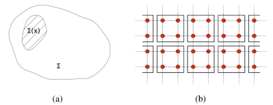
Figure 1: (Color online) (a) The search space for the self-energy $\mathsf{\Sigma}$ is restricted to self-energies $\mathsf{\Sigma}(\mathsf{x})$ which are accessible via the reference system $\hat{H}^{\prime}$. (b) Lattice decomposition of a square lattice into $2\times 2$ site clusters.

In VCA the reference system is given by the decomposition of the total system into identical clusters, see Fig. 1 (b). In order to implement the $\mathsf{Q}$-matrix approach, we solve each cluster by means of the band Lanczos method.Freund (2000); Aichhorn et al. (2006a) The Green’s function of the total system is obtained via the relation

$$\mathsf{G}^{-1}(\omega)=\mathsf{G}^{\prime\,-1}(\omega)-\mathsf{V}\;\mbox{,}$$ (6)

which can be deduced from the Dyson equation of the total system $\mathsf{G}^{-1}=\mathsf{G}_{0}^{-1}-\mathsf{\Sigma}(\mathsf{x})$ and the reference system $\mathsf{G}^{\prime\,-1}=\mathsf{G}_{0}^{\prime\,-1}-\mathsf{\Sigma}(\mathsf{x})$. The self-energy can be eliminated and it follows that

$$\mathsf{G}^{-1}=\mathsf{G}^{\prime\,-1}-(\mathsf{G}^{\prime\,-1}_{0}-\mathsf{G}^{-1}_{0})\;\mbox{.}$$

The expression in parenthesis defines the matrix

$$\mathsf{V} \equiv\mathsf{G}^{\prime\,-1}_{0}-\mathsf{G}^{-1}_{0}=((\omega+\mu^{\prime})\hat{\mathbbm{1}}-\mathsf{T}^{\prime})-((\omega+\mu)\hat{\mathbbm{1}}-\mathsf{T})$$

$$=-(\mu-\mu^{\prime})\hat{\mathbbm{1}}+(\mathsf{T}-\mathsf{T}^{\prime})\;\mbox{.}$$ (7)

With Eq. (6) the grand potential $\Omega(\mathsf{x})$ can be rewritten as

$$\Omega(\mathsf{x})=\Omega^{\prime}(\mathsf{x})+\mbox{Tr}\ln(\hat{\mathbbm{1}}-\mathsf{V}\mathsf{G}^{\prime})\;\mbox{.}$$ (8)

The decomposition of the $N$-site lattice into clusters of $L$ sites can be described by a superlattice. The original lattice is obtained by attaching a cluster to each site of the superlattice.Sénéchal (2008) A partial Fourier transform from superlattice indices to wave vectors ${\bf\tilde{k}}$, which belong to the first Brillouin zone of the superlattice, yields the total Green’s function

$$\mathsf{G}^{-1}({\bf\tilde{k}},\,\omega)=\mathsf{G}^{\prime\,-1}(\omega)-\mathsf{V}({\bf\tilde{k}})\;\mbox{.}$$ (9)

Due to the diagonality of $\mathsf{G}^{\prime}$ in the superlattice indices its partial Fourier transform does not depend on ${\bf\tilde{k}}$. The matrices in Eq. (9) are now defined in the space of cluster-site indices and are thus of size $L\times L$. The $N$ wave vectors ${\bf k}$ from the Brillouin zone of the total lattice can be expressed as

$${\bf k}={\bf\tilde{k}}+{\bf K}\;\mbox{,}$$ (10)

where ${\bf K}$ belongs to both the reciprocal superlattice and the first Brillouin zone of the total lattice.Sénéchal (2008)

III.2 $\mathsf{Q}$-matrix formalism for bosonic systems

The frequency integration implicit in the expression for the grand potential, given in Eq. (8), can be carried out analytically, yielding at zero temperatureKoller and Dupuis (2006); Potthoff (2003b); Sénéchal (2008)

$$\Omega(\mathsf{x})=\Omega^{\prime}(\mathsf{x})+\sum_{\lambda_{r}^{\prime}<0}\lambda_{r}^{\prime}-\frac{1}{N_{c}}\sum_{\bf\tilde{k}}\sum_{\lambda_{r}({\bf\tilde{k}})<0}\lambda_{r}({\bf\tilde{k}})\;\mbox{,}$$ (11)

where $\lambda_{r}^{\prime}$ and $\lambda_{r}({\bf\tilde{k}})$ are the poles of the cluster Green’s function and total Green’s function, respectively. The number of clusters $N/L$ is denoted as $N_{c}$. The poles $\lambda_{r}^{\prime}$ of the cluster Green’s function can be readily obtained from the Lanczos method, whereas the poles of the total Green’s function $\lambda_{r}({\bf\tilde{k}})$ can be evaluated with the so-called $\mathsf{Q}$-matrix formalism, which was originally proposed for fermionic Green’s functions.Aichhorn et al. (2006a); Zacher et al. (2002) Here, we extend this formalism to the generic case, i. e., we include bosonic Green’s functions. As we will see, this extension is nontrivial, since it involves non-unitary transformations.

For zero temperature, the cluster Green’s function reads Fetter and Walecka (1971)

$$G_{ij}^{\prime}\left(\omega\right) =\mathinner{\langle{\psi_{0}}|}a_{i}\frac{1}{\omega-(\hat{H}^{\prime}-\omega_{0})}a_{j}^{\dagger}\mathinner{|{\psi_{0}}\rangle}$$

$$-\epsilon\mathinner{\langle{\psi_{0}}|}a_{j}^{\dagger}\frac{1}{\omega+(\hat{H}^{\prime}-\omega_{0})}a_{i}\mathinner{|{\psi_{0}}\rangle}\;\mbox{,}$$ (12)

where $\mathinner{|{\psi_{0}}\rangle}$ is the ground state of the $N_{p}$ particle system, $\omega_{0}$ is its (grand-canonical) energy, and $\epsilon=1$ ($\epsilon=-1$) for bosonic (fermionic) Green’s functions. The first term on the right-hand side of Eq. (12) describes single-particle excitations from the $N_{p}$ particle ground state and can thus be referred to as particle term, whereas the second part corresponds to single-hole excitations and can be called hole term. Inserting the identity $\hat{\mathbbm{1}}=\sum_{\gamma}\mathinner{|{\gamma}\rangle}\mathinner{\langle{\gamma}|}$ into each part of Eq. (12), where $\mathinner{|{\gamma}\rangle}$ are the eigenvectors of the reference Hamiltonian with corresponding eigenvalues $\omega^{\prime}_{\gamma}$, yields the Lehmann representation of the Green’s function

$$G^{\prime}_{ij}\left(\omega\right) =\sum_{\alpha}\frac{\mathinner{\langle{\psi_{0}}|}a_{i}\mathinner{|{\alpha}\rangle}\mathinner{\langle{\alpha}|}a_{j}^{\dagger}\mathinner{|{\psi_{0}}\rangle}}{\omega-\left(\omega_{\alpha}^{\prime}-\omega_{0}\right)}$$

$$-\epsilon\sum_{\beta}\frac{\mathinner{\langle{\psi_{0}}|}a_{j}^{\dagger}\mathinner{|{\beta}\rangle}\mathinner{\langle{\beta}|}a_{i}\mathinner{|{\psi_{0}}\rangle}}{\omega+\left(\omega_{\beta}^{\prime}-\omega_{0}\right)}\;\mbox{,}$$ (13)

which can be cast into the form

$$G^{\prime}_{ij}\left(\omega\right)=\sum_{\gamma}Q_{i\gamma}\frac{1}{\omega-\lambda_{\gamma}^{\prime}}S_{\gamma\gamma}Q_{\gamma j}^{\dagger}\;\mbox{.}$$ (14)

In Eq. (14), we have introduced the following notation:

$$Q_{\gamma j}^{\dagger}\equiv\left\{\begin{array}[]{ccc}\mathinner{\langle{\gamma}|}a_{j}^{\dagger}\mathinner{|{\psi_{0}}\rangle}&&\mathinner{|{\gamma}\rangle}\in\mathcal{H}_{N_{p}+1}\\ \mathinner{\langle{\psi_{0}}|}a_{j}^{\dagger}\mathinner{|{\gamma}\rangle}&&\mathinner{|{\gamma}\rangle}\in\mathcal{H}_{N_{p}-1}\end{array}\right.\;\mbox{,}$$ (15)

$$\lambda_{\gamma}^{\prime}\equiv\left\{\begin{array}[]{ccc}\omega_{\gamma}^{\prime}-\omega_{0}&&\mathinner{|{\gamma}\rangle}\in\mathcal{H}_{N_{p}+1}\\ \omega_{0}-\omega_{\gamma}^{\prime}&&\mathinner{|{\gamma}\rangle}\in\mathcal{H}_{N_{p}-1}\end{array}\right.$$ (16)

and

$$S_{\gamma\gamma^{\prime}}\equiv\left\{\begin{array}[]{ccl}\delta_{\gamma\gamma^{\prime}}&&\mathinner{|{\gamma}\rangle}\in\mathcal{H}_{N_{p}+1}\\ -\epsilon\,\delta_{\gamma\gamma^{\prime}}&&\mathinner{|{\gamma}\rangle}\in\mathcal{H}_{N_{p}-1}\end{array}\right.\;\mbox{,}$$ (17)

where $\mathcal{H}_{M}$ is the Hilbert space of an $M$ particle system. With

$$g^{\prime}_{\gamma\gamma^{\prime}}\left(\omega\right)\equiv\frac{\delta_{\gamma\gamma^{\prime}}}{\omega-\lambda_{\gamma}^{\prime}}$$ (18)

the cluster Green’s function can be written in matrix notation

$$\mathsf{G}^{\prime}\equiv\mathsf{Q}\,\mathsf{g}^{\prime}\left(\omega\right)\,\mathsf{S}\,\mathsf{Q}^{\dagger}\;\mbox{.}$$ (19)

With the help of this expression the VCA Green’s function Eq. (9) can be rewritten as

$$\mathsf{G} =\mathsf{G}^{\prime}\frac{1}{1-\mathsf{V}\,\mathsf{G}^{\prime}}=\mathsf{Q}\,\mathsf{g}^{\prime}\,\mathsf{S}\,\mathsf{Q}^{\dagger}\frac{1}{1-\mathsf{V}\,\mathsf{Q}\,\mathsf{g}^{\prime}\,\mathsf{S}\,\mathsf{Q}^{\dagger}}$$

$$=\mathsf{Q}\,\mathsf{g}^{\prime}\,\mathsf{S}\,\mathsf{Q}^{\dagger}\left\{1+\mathsf{V}\,\mathsf{Q}\,\mathsf{g}^{\prime}\,\mathsf{S}\,\mathsf{Q}^{\dagger}+\ldots\right\}$$

$$=\mathsf{Q}\,\mathsf{g}^{\prime}\left[1-\mathsf{S}\,\mathsf{Q}^{\dagger}\,\mathsf{V}\,\mathsf{Q}\,\mathsf{g}^{\prime}\right]^{-1}\mathsf{S}\,\mathsf{Q}^{\dagger}$$

$$=\mathsf{Q}\frac{1}{\mathsf{g}^{\prime\,-1}-\mathsf{S}\,\mathsf{Q}^{\dagger}\,\mathsf{V}\,\mathsf{Q}}\mathsf{S}\,\mathsf{Q}^{\dagger}\;\mbox{,}$$ (20)

where in the third step we expanded the fraction in a Taylor series. The matrix $\mathsf{g}^{\prime}$ is diagonal and contains the poles of the cluster Green’s function $\mathsf{G}^{\prime}$, see Eq. (18). It can be written as $\mathsf{g}^{\prime\,-1}=\omega-\mathsf{\Lambda}$ with $\Lambda_{\gamma\gamma^{\prime}}=\lambda_{\gamma}^{\prime}\,\delta_{\gamma\gamma^{\prime}}$. Plugging this into Eq. (20) yields

$$\mathsf{G}=\mathsf{Q}\frac{1}{\omega-(\mathsf{\Lambda}+\mathsf{S}\,\mathsf{Q}^{\dagger}\,\mathsf{V}\,\mathsf{Q})}\mathsf{S}\,\mathsf{Q}^{\dagger}\;\mbox{.}$$ (21)

We introduce the matrix $\mathsf{M}\equiv\mathsf{\Lambda}+\mathsf{S}\,\mathsf{Q}^{\dagger}\,\mathsf{V}\,\mathsf{Q}$. This matrix can be diagonalized as $\mathsf{M}\mathsf{X}=\mathsf{X}\mathsf{D}$, where $\mathsf{D}$ is a diagonal matrix containing the eigenvalues of $\mathsf{M}$ and $\mathsf{X}$ is the matrix of the eigenvectors of $\mathsf{M}$. The eigenvalue equation of the matrix $\mathsf{M}$ can be rewritten as $\mathsf{M}=\mathsf{X}\mathsf{D}\mathsf{X}^{-1}$, where $\mathsf{X}^{-1}$ is the inverse of $\mathsf{X}$ and not its transpose as $\mathsf{M}$ is a non-symmetric matrix. From that we obtain

$$(\omega-\mathsf{M})^{-1}=\mathsf{X}(\omega-\mathsf{D})^{-1}\mathsf{X}^{-1}\;\mbox{.}$$ (22)

Therefore, the poles of the total Green’s function $\mathsf{G}$ in Eq. (21) are the eigenvalues of the matrix $\mathsf{M}$. The matrices $\mathsf{G}$ and $\mathsf{V}$ are defined on the space of cluster-site indices. Thus $\mathsf{G}$ and $\mathsf{V}$ are of size $L\times L$ and depend on the wave vector $\tilde{{\bf k}}$, see Eq. (9). The matrix $\mathsf{Q}$ is of size $L\times K$, where $K$ is the dimension of the Krylov space generated in the band Lanczos method. Due to the dependence of $\mathsf{V}$ on $\tilde{{\bf k}}$ the diagonalization of the matrix $\mathsf{M}$ yields $K$ eigenvalues $D_{rr^{\prime}}=\lambda_{r}(\tilde{{\bf k}})\,\delta_{rr^{\prime}}$, which are used in Eq. (11). The diagonalization has to be repeated for all wave vectors $\tilde{{\bf k}}$. With that the grand potential $\Omega(\mathsf{x})$ can be evaluated. The crucial point is that for bosonic Green’s functions, the entries of the diagonal matrix $\mathsf{S}$ can be both $1$ as well as $-1$, see Eq. (17). Therefore, the eigenvalue problem is not symmetric.com

The factorization of the total lattice into clusters breaks the translational symmetry of the lattice. Hence the total Green’s function would depend on two wave vectors ${\bf k}$ and ${\bf k}^{\prime}$, which is certainly not correct for a periodic lattice. This has to be circumvented by a periodization prescription that provides a total Green’s function $G({\bf k},\,\omega)$ depending only on one wave vector ${\bf k}$. The periodization prescription proposed in Ref. Sénéchal et al., 2000 (Green’s-function periodization) reads as follows:

$$G({\bf k},\,\omega)=\frac{1}{L}\sum_{\alpha\beta}e^{-i\,{\bf k}\,\left({\bf r}_{\alpha}-{\bf r}_{\beta}\right)}G_{\alpha\beta}({\bf\tilde{k}},\,\omega)\;\mbox{,}$$ (23)

where ${\bf k}$ is a wave vector of the total lattice and ${\bf r}_{\alpha}$ refers to lattice sites $\alpha$ of the cluster. The wave vectors ${\bf\tilde{k}}$ in Eq. (23) can be replaced by the total wave vectors ${\bf k}$ as they just differ by a reciprocal superlattice wave vector, see Eq. (10). With Eqs. (21) and (22) the periodized Green’s function can be rewritten in matrix notation

$$G({\bf k},\,\omega)={\bf v}_{\bf k}^{\dagger}\,\mathsf{Q}\,\mathsf{X}\,(\omega-\mathsf{D})^{-1}\,\mathsf{X}^{-1}\,\mathsf{S}\,\mathsf{Q}^{\dagger}\,{\bf v}_{\bf k}\;\mbox{,}$$ (24)

where the vector ${\bf v}_{\bf k}$ and its adjoint ${\bf v}_{\bf k}^{\dagger}$ contain $L$ plane waves

$${\bf v}_{\bf k}^{\dagger}\equiv\frac{1}{\sqrt{L}}\,\left(e^{-i\,{\bf k}\,{\bf r}_{0}},\,e^{-i\,{\bf k}\,{\bf r}_{1}},\,\ldots\,e^{-i\,{\bf k}\,{\bf r}_{L-1}}\right)\;\mbox{.}$$

There exists as well an alternative periodization prescription where the self-energy $\mathsf{\Sigma}$ is periodized.Koller and Dupuis (2006) This self-energy periodization should prevent spurious gaps, which arise in the spectral function. However, at least for fermion systems, this procedure yields spurious metallic bands in the Mott phase for arbitrarily large $U$. Since we do not observe any spurious gaps in the spectral function of the 2D BH model we use the periodization on the Green’s function defined in Eq. (23).

With the wave-vector resolved Green’s function of the total system $G({\bf k},\,\omega)$ we are able to calculate the single-particle spectral function

$$A({\bf k},\,\omega)\equiv-\frac{1}{\pi}\mbox{Im}\,G({\bf k},\,\omega)\;\mbox{,}$$ (25)

the density of states

$$N(\omega)\equiv\int A({\bf k},\,\omega)\,d{\bf k}=\frac{1}{N}\sum_{{\bf k}}A({\bf k},\,\omega)$$ (26)

and the momentum distribution

$$n({\bf k})\equiv-\int_{-\infty}^{0}A({\bf k},\,\omega)\,d\omega\;\mbox{.}$$

The frequency integration can be evaluated directly by means of the $\mathsf{Q}$-matrix formalism, which yields a sum of the residues of the Green’s function, see Eq. (24), corresponding to negative poles $\lambda_{r}({\bf k})<0$,

$$n({\bf k})=\sum_{\lambda_{r}({\bf k})<0}({\bf v}_{\bf k}^{\dagger}\,\mathsf{Q}\,\mathsf{X})_{r}\,(\mathsf{X}^{-1}\,\mathsf{S}\,\mathsf{Q}^{\dagger}\,{\bf v}_{\bf k})_{r}\;\mbox{.}$$ (27)

IV Results

The BH model exhibits a quantum phase transition from a Mott to a superfluid phase when the ratio between the hopping strength and the on-site repulsion $t/U$ is increased or when particles are added to or removed from the system. The Mott phase is characterized by an integer particle density, a gap in the spectral function and zero compressibility.Fisher et al. (1989)

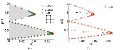
Figure 2: (Color online) Phase boundaries of the Mott phase of the 2D BH model (Mott lobes). (a) Results of our VCA calculation with various cluster sizes for the reference system. The geometry of the 8-site cluster is visualized in the inset. The gray shaded area indicates the results of the process chain approach.Teichmann et al. (2009a, b) (b) Phase boundaries obtained for the 8 site cluster. The marks refer to the parameters where we evaluated the spectral functions.

The first two Mott lobes of the 2D BH model obtained by means of VCA are shown in Fig. 2. We used the chemical potential $\mathsf{x}=\{\mu\}$ as variational parameter, which ensures a correct particle density of the total system.Koller and Dupuis (2006); Aichhorn et al. (2006b) In contrast to the one-dimensional results Koller and Dupuis (2006); Kühner et al. (2000) the Mott lobes of the 2D BH model are round shaped. The gray shaded area in Fig. 2 (a) presents the phase boundaries calculated within the process chain approach by N. Teichmann et al. in Refs. Teichmann et al., 2009a and Teichmann et al., 2009b, which are basically identical to the QMC results by B. Capogrosso-Sansone et al., see Ref. Capogrosso-Sansone et al., 2008. The agreement is quite good for small hopping. However, VCA seems to overestimate the critical value of the hopping $(t/U)_{c}$, which determines the tip of the Mott lobe. For the critical hopping of the first Mott lobe, we obtain approximately $(t/U)_{c}^{1}=0.067$ and for the second one $(t/U)_{c}^{2}=0.038$. Latest process chain approach ,Teichmann et al. (2009a, b) QMC (Ref. Capogrosso-Sansone et al., 2008) and strong-coupling perturbation theory Elstner and Monien (1999) results yield $(t/U)_{c}^{1}=0.059$ and $(t/U)_{c}^{2}=0.035$ for the critical parameter of the first and second Mott lobe, respectively.

The spectral functions $A({\bf k},\,\omega)$ and the densities of states $N(\omega)$ for parameters of the first Mott lobe are shown in Fig. 3.

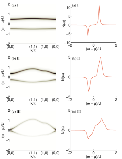
Figure 3: (Color online) Spectral function $A({\bf k},\,\omega)$, left column, and density of states $N(\omega)$, right column, in the first Mott lobe for the parameters (a) $t/U=0.005$, $\mu/U=0.5$, (b) $t/U=0.03$, $\mu/U=0.4$ and (c) $t/U=0.06$, $\mu/U=0.35$. The captions of the subfigures refer to the marks in Fig. 2 (b).

The spectral function is displayed on the conventional path around the Brillouin zone ${\bf k}=(0,0)$ over $(\pi,\pi)$ to $(\pi,0)$ and back to $(0,0)$, and we use an artificial imaginary-frequency broadening $\eta=0.05$. A peculiarity of bosonic systems is that the hole band of the spectral function has negative spectral weight whereas the particle band has positive spectral weight. This follows from the definition of the bosonic Green’s function which has a negative sign in front of the hole term, see Eq. (12). In the figures we always plot the absolute value of the spectral function. The local density of states is defined as a wave-vector summation of $A({\bf k},\,\omega)$, see Eq. (26). Therefore we observe a negative peak in the density of states, which corresponds to the hole band of the spectral function. For bosonic Green’s functions the density of states is not a probability distribution, as it contains negative values. Taking the absolute value would yield an all positive density of states, however, it would not be normed and is thus no probability distribution either. For small hopping, the gap in the spectral function is large and the bands are rather flat, i. e., the width of the bands is small, see Fig. 3. The corresponding density of states contains two well-separated peaks. For increasing hopping, the gap of the spectral function is decreasing and the width of the bands is increasing. Pursuant to the spectral function, the peaks in the density of states become broader for increasing hopping. The intensity of the two bands is almost constant for small hopping independent of the wave vector ${\bf k}$, whereas for large hopping a large intensity can be observed at ${\bf k}={\bf 0}$.

The boundaries of the Mott lobes correspond to the chemical potential of the state with one additional particle (hole), which is obtained directly from the single-particle (single-hole) minimum excitation energy. For this reason, we evaluate the phase diagram in Fig. 2 by taking the minimal gap of the spectral function for each $t/U$, which always occurs at ${\bf k}={\bf 0}$.

The spectral functions and densities of states in the second Mott lobe corresponding to the marks IV and V in Fig. 2 (b) are shown in Fig. 4.

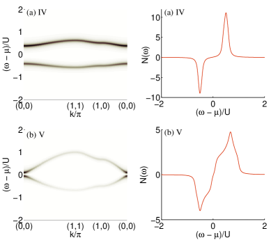
Figure 4: (Color online) Spectral function $A({\bf k},\,\omega)$, left column, and density of states $N(\omega)$, right column, in the second Mott lobe for the parameters (a) $t/U=0.01$, $\mu/U=1.5$ and (b) $t/U=0.035$, $\mu/U=1.4$. The captions of the subfigures refer to the marks in Fig. 2 (b).

Qualitatively they are very similar to the spectral functions and densities of states in the first Mott lobe. Particularly, the intensity distribution of the bands seem to be strongly related. Yet the peaks of the density of states are larger due to the twice as large particle density within the second Mott lobe and thus the absolute value of the spectral weight in the second Mott lobe is larger than the one in the first Mott lobe.

The momentum distribution $n({\bf k})$ corresponding to the spectral functions in the first and second Mott lobe are shown in Fig. 5.

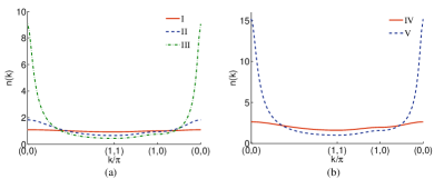
Figure 5: (Color online) Momentum distribution $n({\bf k})$ in (a) the first Mott lobe and (b) the second Mott lobe. The Roman numerals in the legends refer to the parameters marked in Fig. 2 (b).

The particle density in the first Mott lobe is one and thus $n({\bf k})$ is centered around one in Fig. 5 (a). For the second Mott lobe $n({\bf k})$ is centered around two, see Fig. 5 (b). The particle density $n({\bf k})$ is extremely flat for small hopping whereas it is peaked at ${\bf k}={\bf 0}$ for large hopping, which is already a precursor for the Bose-Einstein condensation where all particles condense in the ${\bf k}={\bf 0}$ state. This behavior directly reflects the intensity distribution of the bands in the spectral function. There is excellent quantitative agreement between our VCA results for the momentum distribution and results obtained by means of QMC and a strong-coupling perturbation theory with scaling ansatz,Freericks et al. (2009) see Fig. 6.

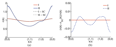
Figure 6: (Color online) Direct comparison (a) between the momentum distribution $n({\bf k})$ obtained by means of VCA and a strong-coupling perturbation theory with scaling ansatz.Freericks et al. (2009) The data identified with the letters SC correspond to the strong-coupling results. The relative deviations between VCA results and strong-coupling results with scaling ansatz are shown in (b). The Roman numerals in the legends refer to the parameters marked in Fig. 2 (b).

We compare the momentum distributions for the parameters I ($t/U=0.005$) and II ($t/U=0.03$), and observe that the relative deviations between our VCA results and an approach obtained by combining strong-coupling perturbation theory with a scaling ansatz Freericks et al. (2009) are almost zero for small hopping $t/U=0.005$ and less than one percent for medium hopping $t/U=0.03$. This latter methods is certainly more accurate than VCA in the evaluation of the momentum distribution. However, it should be mentioned that the information about the critical point (critical exponents and critical hopping strength $(t/U)_{c}$) have to be inserted “by hand,” in order to optimize the results. This information, in turn, must be extracted, e. g., from a QMC calculation. On the other hand, our VCA results are obtained directly without the need to introduce external parameters.

V Conclusions

In the present paper, we presented and discussed results obtained within the variational cluster approach for the spectral properties of the two-dimensional Bose-Hubbard Hamiltonian. This is a minimal model to describe bosonic ultracold atoms confined in optical lattices,Jaksch et al. (1998) and it undergoes a quantum phase transition from a Mott to a superfluid phase depending on the chemical potential $\mu$, and the ratio between the hopping strength and the on-site repulsion $t/U$. In particular, we determined the first two Mott lobes of the phase diagram and found reasonable agreement with essentially exact results from QMC simulations and from the process chain approach. In particular, the variational cluster approach yields very good results for the phase boundaries apart from the region close to the lobe tip. Here, strong-coupling expansions and QMC calculations are, clearly, much more accurate. Yet it should be emphasized that the computational effort is considerably lower for VCA than for QMC. Furthermore, we evaluated spectral functions in the first and second Mott lobe. An important aspect of VCA is that the Green’s function of the system is obtained directly in the real frequency domain, which allows for a direct calculation of the spectral function. On the other hand, QMC quite generally provides correlation functions in imaginary time. Imaginary-time correlation functions have to be analytically continued to real frequencies, which is a very ill-conditioned problem, as the data contain statistical errors. In QMC this analytical continuation is best carried out by means of the maximum entropy method. A very accurate dispersion (without spectral weight) has been also obtained by a strong-coupling expansion.Elstner and Monien (1999) The intensity distribution of the spectral weight is similar for the spectral functions of both Mott lobes, leading to an evenly distributed spectral weight for small hopping strengths and to a distribution sharply peaked at ${\bf k}={\bf 0}$ for large hopping strengths. The latter indicates a precursor to the Bose-Einstein condensation occurring above a certain critical hopping. We also evaluated the densities of states and momentum distributions corresponding to the calculated spectral functions. We compared our VCA results for the momentum distribution with strong-coupling perturbation-theory results, where a scaling ansatz has been used, and found excellent quantitative agreement. Finally, as a technical point, we extended the $\mathsf{Q}$-matrix formalism to deal with bosonic Green’s functions, which, in contrast to the fermionic case, produces a non-symmetric eigenvalue problem.