Modeling the non-Markovian, non-stationary scaling dynamics of financial markets

Abstract

A central problem of Quantitative Finance is that of formulating a probabilistic model of the time evolution of asset prices allowing reliable predictions on their future volatility. As in several natural phenomena, the predictions of such a model must be compared with the data of a single process realization in our records. In order to give statistical significance to such a comparison, assumptions of stationarity for some quantities extracted from the single historical time series, like the distribution of the returns over a given time interval, cannot be avoided. Such assumptions entail the risk of masking or misrepresenting non-stationarities of the underlying process, and of giving an incorrect account of its correlations. Here we overcome this difficulty by showing that five years of daily Euro/US-Dollar trading records in the about three hours following the New York market opening, provide a rich enough ensemble of histories. The statistics of this ensemble allows to propose and test an adequate model of the stochastic process driving the exchange rate. This turns out to be a non-Markovian, self-similar process with non-stationary returns. The empirical ensemble correlators are in agreement with the predictions of this model, which is constructed on the basis of the time-inhomogeneous, anomalous scaling obeyed by the return distribution.

1 Introduction

The analysis of many natural and social phenomena is hindered by the fact that one cannot replicate the dynamical evolution of the system under study. This may happen, for instance, for earthquakes scholz_1 , solar flares lu_1 , large eco-systems bjornstad_1 , and financial markets cont_1 . If with a single time series available we try to accommodate the historical data within a stochastic process description, we must assume a priori the existence of some statistical quantities which remain stable over time cont_1 . This entitles us to sample their values at different stages of the historical evolution, rather than at different instances of the process. For example, in the analysis of historical series in Finance it is usual to assume the stationarity of the distribution of return fluctuations and hence to detect their statistical features through sliding time interval empirical sampling. However, the plausible baldovin_1 ; stella_1 ; bassler_1 ; challet_1 ; andreoli_1 nonstationarity of these fluctuations at intervals ranging from minutes to months would drastically alter the relation between some of the stylized empirical facts detected in this way, and the underlying stochastic process. In order to identify the correct model, one has to overcome this difficulty. The breaking of time-translation invariance possibly signalled by increments non-stationarity would represent a challenge in itself, being a genuine manifestation of dynamics out of equilibrium, like the aging properties observed in glassy systems aging_1 .

In order to detect the possible presence of nonstationarity at certain time-scales for the distribution of the increments, one would need to have access to many independent realizations of the same process, repeated under similar conditions. Quite remarkably, high-frequency financial time-series offer an opportunity of this kind, in which it is possible to directly sample an ensemble of histories. In Ref. bassler_1 it has been proposed that when considering high-frequency EUR/USD exchange rate data as recorded during the first three hours of the New York market activity, independent process realizations can tentatively be identified in the daily repetitions of the trading. This gives the interesting possibility of estimating quantities related to ensemble-, rather than time-averages. Here we profit of this opportunity by showing that a proper analysis of the statistical properties of this ensemble of histories naturally leads to the identification and validation of an original stochatic model of market evolution. The main idea at the basis of this model is that the scaling properties of the return distribution are sufficient to fully characterize the process in the time range within which they hold. The same type of model has been recently proposed by some of the present authors to underlie more generally the evolution of financial indices also in cases when only single realizations are available baldovin_1 . In those cases the application of the model is less direct, and rests on suitable assumptions about the relation between the stationarized empirical information obtainable from the historical series and the underlying driving process.

An interesting feature of the model discussed here and in Refs. baldovin_1 ; stella_1 , is that the anomalous scaling of the return PDF enters in its construction on the basis of a property of correlated stability which generalizes the stability of Gaussian PDF’s under independent random variables summation. This correlated stability was shown recently to allow the derivation of novel, constructive limit theorems for the PDF of sums of many strongly dependent random variables obeying anomalous scaling limit . In this perspective, the model we present offers a valid alternative to more standard models of Finance based on Gaussianity and independence. At the same time, the probabilistic framework provided by our modelization presents clear formal analogies and parallels with those standard models.

2 An ensemble of histories based on the returns of the EUR/USD exchange rate

To address the above points, given the EUR/USD exchange rate at time $t$ ($t$ measured in tens of minutes) after 9.00 am New York time, $S(t)$, let us define the return in the interval $[t-T,t]$ as $R(t,T)\equiv\ln S(t)-\ln S(t-T)$, where $t=1,2,\ldots$, $t\geq T$. By storing the daily repetitions of the returns from March 2000 to March 2005, we obtain an ensemble of $M=1,282$ realizations $\left\{r^{l}(t,T)\right\}_{l=1,2,\ldots,M}$ of the discrete-time stochastic process $R(t,T)$, with $t$ ranging in almost three hours after 9.00 am NY time, i.e., $1\leq t\leq 17$. Below, the superscript “$e$” labels quantities empirically determined on the basis of this ensemble. The first key observation is that the empirical second moment $m_{2}^{e}(t,1)\equiv\sum_{l=1}^{M}[r^{l}(t,1)]^{2}/M$ systematically decreases as a function of $t$ in the interval considered (see Fig. 1a). This is a clear indication of return non-stationarity of the underlying process at this time scale. In addition, an analysis of the nonlinear moments $m_{\alpha}^{e}$ of the total return $R(t,t)=\ln S(t)-\ln S(0)$ for $t\geq 1$,

$$m_{\alpha}^{e}(t,t)\equiv\frac{1}{M}\sum_{l=1}^{M}\left|r^{l}(t,t)\right|^{\alpha},\quad\alpha\in\mathbb{R}_{+},$$ (1)

shows that such a nonstationarity is accompanied by an anomalous scaling symmetry. Indeed, to a good approximation one finds $m_{\alpha}(t,t)\sim t^{\alpha D}$ in this range of $t$, where $D\simeq 0.364\ldots$ is essentially independent of $\alpha$ (Fig. 1b). Accordingly, the ensemble histograms for the PDF’s of aggregated returns in the intervals $[0,t]$, $p_{R(t,t)}$, are consistent with the scaling collapse

$$t^{D}\;p_{R(t,t)}\left(t^{D}\;r\right)=g(r)$$ (2)

reported in Fig. 2. The scaling function $g$ identified by such collapse plot is manifestly non-Gaussian. It may also be assumed to be even to a good approximation.

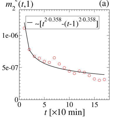
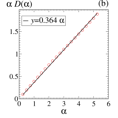
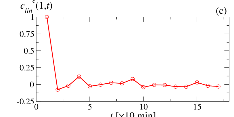
Figure 1: Empirical ensemble analysis of the returns. (a) The line is given by $\langle\sigma^{2}\rangle_{\rho}\;\left[t^{2D}-(t-1)^{2D}\right]$, with $\langle\sigma^{2}\rangle_{\rho}=\langle r_{1}^{2}\rangle_{p}=2.3\cdot 10^{-7}$ and the best-fitted $D=0.358$. (b) Analysis according to the ansatz in Eq. (2). The straight line characterizes a simple-scaling behavior with a best-fitted $D=0.364$. (c) The linear correlation vanishes for non-overlapping returns.

To further simplify our formulas below, wherever appropriate we will switch to the notations: $R_{i}\equiv R(i,1)$ and $r_{i}\equiv r(i,1)$. Similarly $r^{l}_{i}\equiv r^{l}(i,1)$ will indicate the $i$-th return on a $10\;\textrm{min}$-scale in the $l$-th history realization of our ensemble.

An important empirical fact (Fig. 1c) is that the linear correlation between returns for non-overlapping intervals

$$c_{lin}^{e}(1,n)\equiv\frac{\frac{1}{M}\sum_{l=1}^{M}\left[r_{1}^{l}\;r_{n}^{l}\right]}{\sqrt{m_{2}(1,1)\;m_{2}(n,1)}},$$ (3)

with $n=2,\ldots$, is negligible in comparison with the correlation of the absolute values of the same returns. At this time scale also correlators of odd powers of a return with odd or even powers of another return are negligible. Only even powers of the returns are strongly correlated.

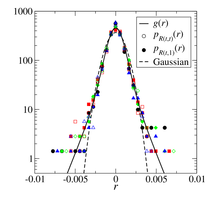
Figure 2: Non-Gaussian scaling function $g$. Empty [full] symbols are obtained by rescaling $p_{R(t,t)}$ [$p_{R(t,1)}$] according to Eq. (2) [Eq. (8)] for $t=1,5,10,17$.

3 Self-similar model process

The empirical facts listed above already enable us to suggest a very plausible model for the stochastic process expected to generate the data. Both in physics and in Finance, a well established trend in modeling anomalous scaling is that of expressing the scaling functions, like our $g$, as convex combinations of Gaussian PDF’s with varying widths. This has clear mathematical advantages, since it is possible to express very general scaling functions with such convex combinations. In physics the representation in terms of mixtures of Gaussians often reflects the presence of some heterogeneity or polydispersity in the problem gheorghiu_1 . In Finance, the use of convex combinations of Gaussians to represent return PDF’s is naturally suggested by the fact that return time series show a variety of more or less long intervals characterized by peculiar values of the volatility (volatility clustering). The idea that $p_{R(t,t)}$ can be represented as a mixture of Gaussians of varying widths is suggested by the same basic motivations which lead to the introduction of stochastic volatility models in Finance bouchaud_1 ; heston_1 ; gatheral_1 ; fouque_1 . In the light of the empirical facts, such a representation of the scaling function in the PDF of the aggregated return naturally suggests an adequate full modelization of the process generating the successive partial returns. Let us indicate by $\rho(\sigma)$ a normalized, positive measure in $]0,+\infty[$ such that we can represent $g$ as:

$$g(x)=\int_{0}^{+\infty}d\sigma\rho(\sigma)\frac{e^{-\frac{x^{2}}{2\sigma^{2}}}}{\sqrt{2\pi\sigma^{2}}}.$$ (4)

A suitable form of $\rho$ can be easily identified, e.g. by matching its moments with those of $g$, and by relating the large $\sigma$ behavior of $\rho(\sigma)$ with the large $|r|$ behavior of $g(r)$. For instance, $\rho$ may decay as a power law at large $\sigma$’s if the moments of $g$ are expected to be infinite above a given order. These conditions enable us to fix a number of parameters in $\rho$ such that the scaling function in Eq. (4) fits the data in the empirical collapse in Fig. 2. As discussed below, in our case the set of data on which we can count to construct histograms of $g$ is relatively poor. So, our determinations of $\rho$ will be rather qualitative.

Once identified $\rho$, more ambitiously we may try to use it for a weighted representation of the joint PDF’s of the successive elementary returns $R_{i}$, $i=1,2,\dots$ generated in the process. Indeed, we may tentatively write the joint PDF of these returns in the following form:

$$p^{n}(r_{1},r_{2},\dots,r_{n})=\int_{0}^{+\infty}d\sigma\rho(\sigma)\prod_{i=1}^{n}\frac{\exp\left({-\frac{r_{i}^{2}}{2\,a_{i}^{2}\,\sigma^{2}}}\right)}{\sqrt{2\pi\,a_{i}^{2}\,\sigma^{2}},}$$ (5)

with $n=1,2,\ldots,17$. The coefficients $a_{i}$ in the last equation have to be chosen consistent with the non-stationarity of the elementary returns reported in Fig. 1a and with the other statistical properties of the elementary and aggregated returns discussed in the previous section. It is straightforward to realize that $\langle r_{i}^{2}\rangle_{p}=\langle\sigma^{2}\rangle_{\rho}\,a_{i}^{2}$, while $\langle r_{i}\rangle_{p}=0$ and $\langle r_{i}r_{j}\rangle_{p}=0$ for $i\neq j$, where $\langle\cdot\rangle_{p}$ denotes averages with respect to the joint PDF in Eq.(5), whereas $\langle\cdot\rangle_{\rho}$ those with respect to the PDF $\rho$. Likewise, we immediately realize that odd-odd or odd-even correlators of the $R_{i}$’s are strictly zero. Assuming validity of Eq. (5) means in first place that the $i$-dependence of $a_{i}$ must be chosen such to fit the values reported in Fig. 1a. The choice of the $i$ dependence of $a_{i}$ must be also consistent with the simple scaling of the PDF of aggregated returns. Indeed, taking into account that $R(t,t)=R_{1}+R_{2}+\dots+R_{t}$, for $t=1,2,\dots,17$, Eq.(5) implies that for the same $t$ values

$$p_{R(t,t)}(r)=\frac{g\left(r/\sqrt{a_{1}^{2}+a_{2}^{2}+\dots+a_{t}^{2}}\right)}{\sqrt{a_{1}^{2}+a_{2}^{2}+\dots+a_{t}^{2}}}.$$ (6)

Comparing this result with Eq. (2), we see that it is necessary to choose the $a_{i}$’s such that $a_{1}^{2}+a_{2}^{2}+\dots+a_{t}^{2}=t^{2D}$ in order to be consistent with the empirical scaling in Eq. (2). This last requirement is satisfied if we put

$$a_{i}=\sqrt{i^{2D}-(i-1)^{2D}},\quad i=1,2,\ldots\;.$$ (7)

A first problem is then to see whether this form of the $a_{i}$ coefficients is compatible with the $i$-dependence already implied by the non-stationarity. Eq. (7) appears to be reasonably well compatible with the trend of the empirical mean square elementary returns $m_{2}(i,1)$. Indeed, given $\langle\sigma^{2}\rangle_{\rho}=\langle r_{1}^{2}\rangle_{p}=2.3\cdot 10^{-7}$, the best fit in Fig. 1a is obtained with $D=0.358\ldots$ in the expression for $\langle r_{i}^{2}\rangle_{p}$. The expectation value of $\sigma^{2}$ is with respect to the $\rho$ entering the integral representation (3) already chosen for $g$. Remarkably, the value of $D$ is very close to the estimate of $D$ obtained above through the analysis of the moments of $p_{R(t,t)}$.

Summarizing, Eq.(5) and the above conditions on the $a_{i}$’s define a non-Markovian stochastic process with linearly uncorrelated increments and a PDF of returns satifying a time inhomogeneous scaling of the form:

$$p_{R(t,T)}(r)=\frac{1}{\sqrt{t^{2D}-(t-T)^{2D}}}\;\;g\left(\frac{r}{\sqrt{t^{2D}-(t-T)^{2D}}}\right),$$ (8)

where both $t$ and $T$ are understood to be integer multiples of the $\rm{10}$ minutes unit. In Fig. 2 it is shown that the data collapse of both $p_{R(t,t)}$ and $p_{R(t,1)}$ are indeed compatible with the same non-gaussian PDF $g$.

From the point of view of probability theory, the structure of our process in Eq.(5) rests on a stability property for PDF’s of sums of dependent random variables limit . Indeed, if we indicate by $\tilde{p}^{n}(k_{1},k_{2},...k_{n})$ the Fourier transform (characteristic function) of the joint PDF of the first $n$ returns ($1\leq n\leq 17$), a direct calculation yields

$$\tilde{p}^{n}(k,k,...,k)=\tilde{p}^{1}\left(n^{D}K\right)$$ (9)

and

$$\tilde{p}^{n}(0,..,k_{i},..,0)=\tilde{p}^{1}(a_{i}k_{i}),\quad i=1,\dots,n.$$ (10)

For $D=1/2$ these relations have the the same form as those holding in the case of independent variables, when $\tilde{p}^{n}(k_{1},\dots,k_{n})=\tilde{p}^{1}(k_{1})\,\tilde{p}^{1}(k_{2})\,\dots\,\tilde{p}^{1}(k_{n})$, and $\tilde{p}^{1}$ is a Gaussian characteristic function. However, even for $D=1/2$ a general $\rho(\sigma)$ implies dependence of the $R_{i}$’s. To recover the independent case one needs further to choose $\rho(\sigma)=\delta(\sigma-\sigma_{0})$. Thus, the superposition of independent Gaussian processes with different $\sigma$’s in Eq.(5) implies an extension of the basic stability properties of the independent Gaussian variables case to the dependent case. This extension also allows to derive limit theorems for the anomalous scaling of sums of many dependent random variables limit .

4 Correlations structure

As discussed above, the identification of $\rho$ may be used to reconstruct the joint PDF of the returns $R_{i}$’s as in Eq. (5). In this section we elaborate further on this point, by performing a detailed comparison between model predictions (based on an explicit expression for $\rho$) and empirical determinations of various two-point correlators.

Considering the data collapse of both $p_{R(t,t)}$ and $p_{R(t,1)}$ in Fig. 2, we propose the following functional form for $\rho$ (see also limit ):

$$\rho(\sigma)=A\;\frac{\sigma^{\gamma}}{d+\sigma^{\delta}},\quad\sigma\in[\sigma_{min},+\infty[,\quad 0<\gamma<\delta,$$ (11)

where $A$ is a normalization factor, and $d>0$ is a parameter influencing the width of the distribution $g$. Notice that $\rho(\sigma)\sim\sigma^{-(\delta-\gamma)}$ for $\sigma\gg 1$. The rational behind this choice for $\rho$ is that one can use the exponents $\gamma,\delta$ to reproduce the large $|x|$ behavior of $g(x)$, and then play with the other parameters to obtain a suitable fit of the scaling function, for instance the one reported in Fig. 2.

The first two-point correlator we consider in our analysis is

$$\kappa_{\alpha,\beta}(1,n)\equiv\frac{\langle\left|R(1,1)\right|^{\alpha}\;\left|R(n,1)\right|^{\beta}\rangle}{\langle\left|R(1,1)\right|^{\alpha}\rangle_{p}\;\langle\left|R(n,1)\right|^{\beta}\rangle_{p}}=\frac{\langle\left|r_{1}\right|^{\alpha}\;\left|r_{n}\right|^{\beta}\rangle_{p}}{\langle\left|r_{1}\right|^{\alpha}\rangle_{p}\;\langle\left|r_{n}\right|^{\beta}\rangle_{p}},$$ (12)

with $n>1$, and $\alpha,\beta\in\mathbb{R}_{+}$. A value $\kappa_{\alpha,\beta}\neq 1$ means that returns on non-overlapping intervals are dependent. Using Eq. (5) it is possible to express a general many-return correlator in terms of the moments of $\rho$. For example, from Eq. (5) we have

$$\langle\left|r_{1}\right|^{\alpha}\;\left|r_{n}\right|^{\beta}\rangle_{p}=B_{\alpha}\,B_{\beta}\;\;a_{1}^{\alpha}\,a_{n}^{\beta}\;\langle\sigma^{\alpha+\beta}\rangle_{\rho},$$ (13)

with

$$B_{\alpha}\equiv\int_{-\infty}^{+\infty}dr\;|r|^{\alpha}\;\frac{e^{-r^{2}/2}}{\sqrt{2\pi}}.$$ (14)

We thus obtain

$$\kappa_{\alpha,\beta}(1,n)=\frac{\langle\sigma^{\alpha+\beta}\rangle_{\rho}}{\langle\sigma^{\alpha}\rangle_{\rho}\;\langle\sigma^{\beta}\rangle_{\rho}}=\frac{B_{\alpha}B_{\beta}}{B_{\alpha+\beta}}\frac{\langle|r_{1}|^{\alpha+\beta}\rangle_{p}}{\langle|r_{1}|^{\alpha}\rangle_{p}\;\langle|r_{1}|^{\beta}\rangle_{p}}.$$ (15)

Two model-predictions in Eq. (15) are: (i) Despite the non-stationarity of the increments $R_{i}$’s, $\kappa_{\alpha,\beta}(1,n)$ is independent of $n$; (ii) The correlators are symmetric, i.e., $\kappa_{\alpha,\beta}-\kappa_{\beta,\alpha}=0$.

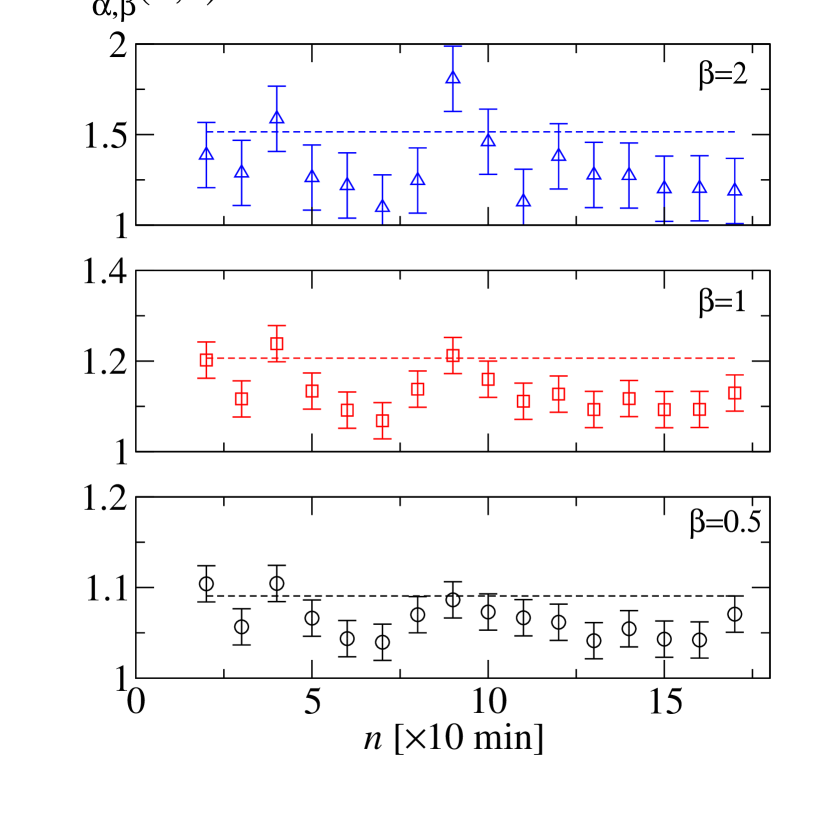
Figure 3: Constancy of $\kappa^{e}_{\alpha,\beta}$. Dashed lines are model-predictions.

We can now compare the theoretical prediction of the model for $\kappa_{\alpha,\beta}(1,n)$, Eq. (15), with the empirical counterpart

$$\kappa^{e}_{\alpha,\beta}(1,n)\equiv\frac{\sum_{l=1}^{M}\left[\left|r_{1}^{l}\right|^{\alpha}\;\left|r_{n}^{l}\right|^{\beta}\right]}{\frac{1}{M}\sum_{l=1}^{M}\left|r_{1}^{l}\right|^{\alpha}\;\sum_{l=1}^{M}\left|r_{n}^{l}\right|^{\beta}},$$ (16)

which we can calculate from the EUR/USD dataset. Notice that once $\rho$ is fixed to fit the one-time statistics in Fig. 2, in this comparison we do not have any free parameter to adjust. Also, since our ensemble is restricted to $M=1,282$ realizations only, large fluctuations, especially in two-time statistics, are to be expected.

Fig. 3 shows that indeed non-overlapping returns are strongly correlated in the about three hours following the opening of the trading session, since $\kappa^{e}_{\alpha,\beta}\neq 1$. In addition, the constancy of $\kappa^{e}_{\alpha,\beta}$ is clearly suggested by the empirical data. In view of this constancy, we can assume as error-bars for $\kappa^{e}_{\alpha,\beta}$ the standard deviations of the sets $\left\{\kappa^{e}_{\alpha,\beta}(1,n)\right\}_{n=2,3,\ldots,17}$. The empirical values for $\kappa^{e}_{\alpha,\beta}$ are also in agreement with the theoretical predictions for $\kappa_{\alpha,\beta}$ based on our choice for $\rho$. In this and in the following comparisons it should be kept in mind that, although not explicitly reported in the plots, the uncertainty in the identification of $\rho$ of course introduces an uncertainty in the model-predictions for the correlators.

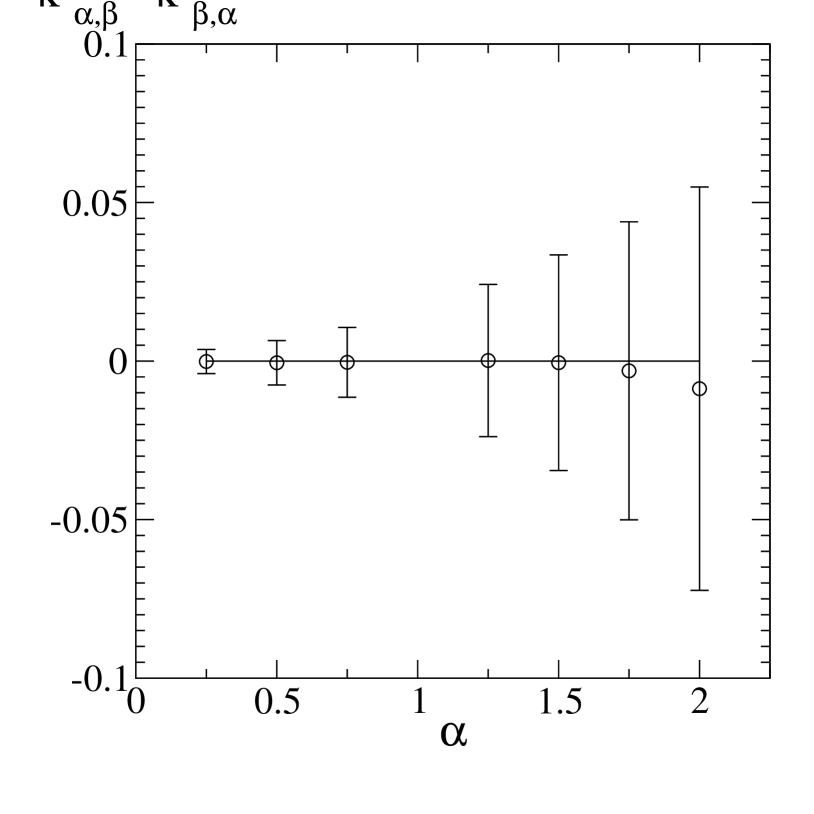
Figure 4: Symmetry of $\kappa^{e}_{\alpha,\beta}$. Error-bars are determined as in Fig. 3.

In Fig. 4 we report that also the symmetry $\kappa_{\alpha,\beta}=\kappa_{\beta,\alpha}$ is emiprically verified for the EUR/USD dataset. The validity of this symmetry for a process with non-stationary increments like the present one is quite remarkable.

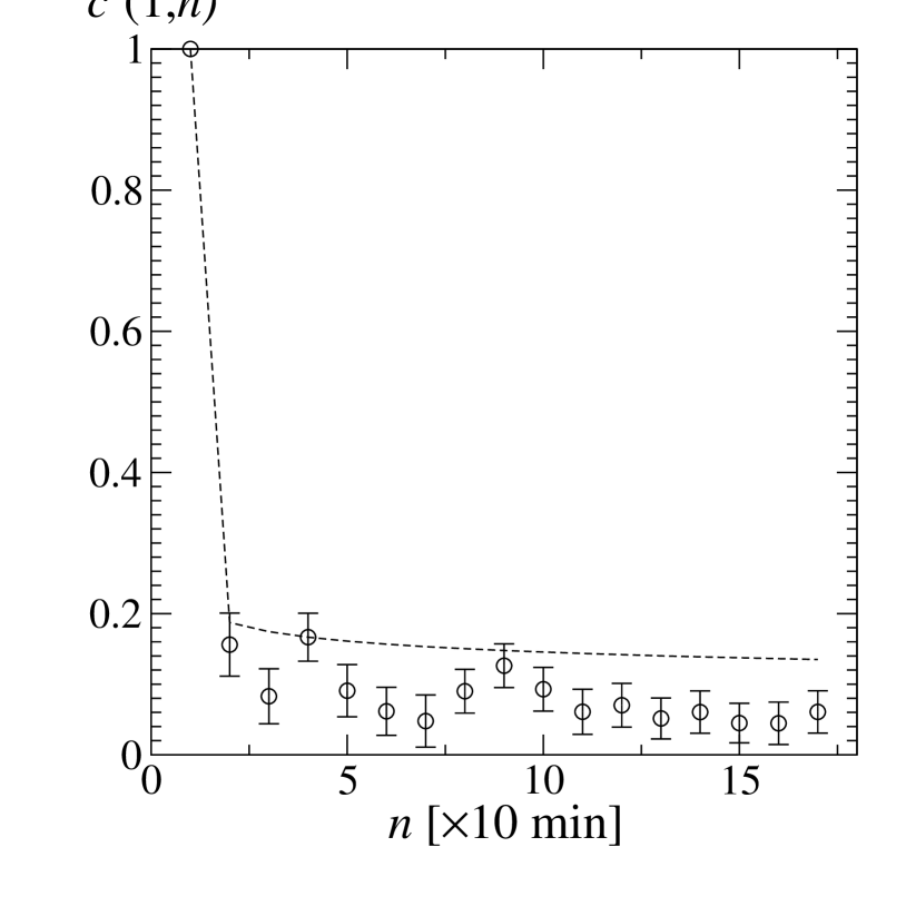
Figure 5: Volatility autocorrelation. Dashed line is the model-prediction.

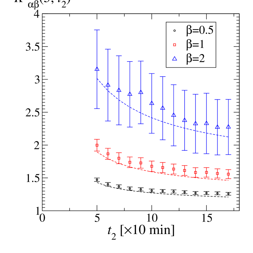
Figure 6: Correlators $K^{e}_{\alpha,\beta}$. Dashed lines are model-predictions.

A classical indicator of strong correlations in financial data is the volatility autocorrelation, defined as

$$c(1,n)\equiv\frac{\langle\left|r_{1}\right|\;\left|r_{n}\right|\rangle_{p}-\langle\left|r_{1}\right|\rangle_{p}\;\langle\left|r_{n}\right|\rangle_{p}}{\langle\left|r_{1}\right|^{2}\rangle_{p}\;-\langle\left|r_{1}\right|\rangle_{p}^{2}}.$$ (17)

In terms of the moments of $\rho$, through Eq. (13) we have the following expression for $c$ :

$$c(1,n)=\frac{B_{1}^{2}\;a_{1}\;a_{n}\;\left[\langle\sigma^{2}\rangle_{\rho}-\langle\sigma\rangle_{\rho}^{2}\right]}{a_{1}^{2}\;\left[B_{2}\;\langle\sigma^{2}\rangle_{\rho}-B_{1}^{2}\langle\sigma\rangle_{\rho}^{2}\right]}.$$ (18)

Unlike $\kappa_{\alpha,\beta}$, $c$ is not constant in $n$. The comparison with the empirical volatility autocorrelation,

$$c^{e}(1,n)\equiv\frac{\sum_{l=1}^{M}\left[\left|r_{1}^{l}\right|\;\left|r_{n}^{l}\right|\right]-\frac{1}{M}\sum_{l=1}^{M}\left|r_{1}^{l}\right|\;\sum_{l^{\prime}=1}^{M}\left|r_{n}^{l^{\prime}}\right|\;}{\sum_{l=1}^{M}\left|r_{1}^{l}\right|^{2}-\frac{1}{M}\sum_{l=1}^{M}\left|r_{1}^{l}\right|\;\sum_{l^{\prime}=1}^{M}\left|r_{1}^{l^{\prime}}\right|\;},$$ (19)

yields a substantial agreement (See Fig. 5). The error-bars in Fig. 5 are obtained by dynamically generating many ensembles of $M=1,282$ realizations each, according to Eq. (5) with our choice for $\rho$, and taking the standard deviations of the results. Again, the uncertainty associated to the theoretical prediction for $c$ is not reported in the plots Problems concerning the numerical simulation of processes like the one in Eq. (5) are discussed in Ref. limit .

A further test of our model can be made by analyzing, in place of those of the increments, the non-linear correlators of $R(t,t)$, with varying $t$. To this purpose, let us define

$$K_{\alpha,\beta}(t_{1},t_{2})\equiv\frac{\langle\left|R(t_{1},t_{1})\right|^{\alpha}\;\left|R(t_{2},t_{2})\right|^{\beta}\rangle}{\langle\left|R(t_{1},t_{1})\right|^{\alpha}\rangle\;\langle\left|R(t_{2},t_{2})\right|^{\beta}\rangle},$$ (20)

with $t_{2}\geq t_{1}$. Model calculations similar to the previous ones give, from Eq. (5),

$$K_{\alpha,\beta}(t_{1},t_{2})=\frac{B_{\alpha,\beta}^{(2)}(t_{1},t_{2})}{t_{1}^{\alpha D}t_{2}^{\beta D}B_{\alpha+\beta}}\frac{\langle\left|r_{1}\right|^{\alpha+\beta}\rangle_{p}}{\langle\left|r_{1}\right|^{\alpha}\rangle_{p}\;\langle\left|r_{1}\right|^{\beta}\rangle_{p}},$$ (21)

where

$$B_{\alpha,\beta}^{(2)}(t_{1},t_{2})\equiv\int_{-\infty}^{+\infty}dr_{1}\;|r_{1}|^{\alpha}\;\frac{\exp\left(-r_{1}^{2}/\left(2t_{1}^{2D}\right)\right)}{\sqrt{2\pi t_{1}^{2D}}}$$

$$\int_{-\infty}^{+\infty}dr_{2}\;|r_{2}|^{\beta}\;\frac{\exp\left[-(r_{1}-r_{2})^{2}/\left(2t_{2}^{2D}-2t_{1}^{2D}\right)\right]}{\sqrt{2\pi\left(t_{2}^{2D}-t_{1}^{2D}\right)}}.$$ (22)

According to Eq. (21), $K_{\alpha,\beta}$ is now identified by both $\rho$ and $D$. Moreover, it explicitly depends on $t_{1}$ and $t_{2}$. The comparison between Eq. (21) and the empirical quantity

$$K^{e}_{\alpha,\beta}(t_{1},t_{2})\equiv\frac{\sum_{l=1}^{M}\left[\left|r^{l}(t_{1},t_{1})\right|^{\alpha}\;\left|r^{l}(t_{2},t_{2})\right|^{\beta}\right]}{\frac{1}{M}\sum_{l=1}^{M}\left[\left|r^{l}(t_{1},t_{1})\right|^{\alpha}\right]\;\sum_{l=1}^{M}\left[\left|r^{l}(t_{2},t_{2})\right|^{\beta}\right]},$$ (23)

reported in Fig. 6 (the error-bars are determined as in Fig. 5) supplies thus an additional validation of our model.

5 Conclusions

In the present work we addressed the problem of describing the time evolution of financial assets in a case in which one can try to compare the predictions of the proposed model with a relatively rich ensemble of history realizations. Besides the fact that considering the histories at disposal for the EUR/USD exchange rate as a proper ensemble amounts to a main working assumption, a clear limitation of such an approach is the relative poorness of the ensemble itself. Indeed, the simulations of our model suggest that in order to reduce substantially the statistical fluctuations one should dispose of ensembles larger by at least one order of magnitude.

In spite of these limitations, we believe that the non-Markovian model we propose baldovin_1 ; stella_1 ; limit is validated to a reasonable extent by the analysis of the data, especially those pertaining to the various correlators we considered. In this respect it is important to recall that the first proposal of the time inhomogeneous evolution model discussed here has been made in a study of a single, long time series of the DJI index in Ref. baldovin_1 . In that context, the returns time inhomogeneity, Eq. (8), was supposed to underlie the stationarized information provided by the empirical PDF of the returns. This assumption allowed there to give a justification of several stylized facts, like the scaling and multiscaling of the empirical return PDF and the power law behavior in time of the return autocorrelation function. We believe that the results obtained in the present report, even if pertaining to a different time-scale (tens of minutes in place of days), constitute an interesting further argument in favor of a general validity of the model.

The peculiar feature of this model is that of focussing on scaling and correlations as basic, closely connected properties of assets evolution. This was strongly inspired by what has been learnt in the physics of complex systems in the last decades kadanoff_1 ; kadanoff_2 ; lasinio_1 , where methods like the renormalization group allowed for the first time systematic treatments of these properties stella_1 . At the same time, through the original probabilistic parallel mentioned in Section 3, our model maintains an interesting direct contact with the mathematics of standard formulations based on Brownian motion, of wide use in Finance. This last feature is very interesting in the perspective of applying our model to problems of derivative pricing bouchaud_1 ; heston_1 ; gatheral_1 ; fouque_1 ; black_1 .

Acknowledgments
We thank M. Caporin for useful discussions. This work is supported by “Fondazione Cassa di Risparmio di Padova e Rovigo” within the 2008-2009 “Progetti di Eccellenza” program.

References

- (1) Scholz CH (2002) The Mechanics of Earthquakes and Faulting. Cambridge University Press, New York.
- (2) Lu ET, Hamilton RJ, McTiernan JM, Bromond KR (1993) Solar flares and avalanches in driven dissipative systems. Astrophys. J. 412: 841–852
- (3) Bjornstad ON, Grenfell BT (2001) Noisy clockwork: time series analysis of population fluctuations in animals. Science 293: 638–643
- (4) Cont R (2001) Empirical properties of asset returns: stylized facts and statistical issues. Quant. Finance 1: 223–236.
- (5) Baldovin F, Stella AL (2007) Scaling and efficiency determine the irreversible evolution of a market. Proc. Natl. Acad. Sci. 104: 19741–19744
- (6) Stella AL, Baldovin F (2008) Role of scaling in the statistical modeling of Finance. Pramana - Journal of Physics 71, 341–352
- (7) Bassler KE, McCauley JL, Gunaratne GH (2007) Nonstationary increments, scaling distributions, and variable diffusion processes in financial markets. Proc. Natl. Acad. Sci. USA 104: 17287-17290
- (8) D. Challet and P.P. Peirano (2008) The ups and downs of the renormalization group applied to financial time series. arXiv:0807.4163
- (9) A. Andreoli, F. Caravenna, P. Dai Pra, G. Posta (2010) Scaling and multiscaling in financial indexes: a simple model. arXiv:1006.0155
- (10) De Benedetti PG, Stillinger FH (2001) Supercooled liquids and the glass transition. Nature 410: 259–267
- (11) Stella AL, Baldovin F (2010) Anomalous scaling due to correlations: Limit theorems and self-similar processes. J. Stat. Mech. P02018.
- (12) Gheorghiu S, Coppens MO (2004) Heterogeneity explains features of “anomalous” thermodynamics and statistics. Proc. Natl. Acad. Sci. USA 101: 15852–15856.
- (13) Bouchaud JP, Potters M (2000) Theory of Financial Risks Cambridge University Press, Cambridge, UK.
- (14) Heston L (1993) A Closed-Form Solution for Options with Stochastic Volatility with Applications to Bond and Currency Options. The Review of Financial Studies 6: 327-343
- (15) Gatheral J (2006) The volatility surface: a practitioner’s guide. J. Wiley and Sons, New Jersey
- (16) Fouque JP, Papanicolaou G, Sircar KR (2000) Derivatives in financial markets with stochastic volatility. Cambridge University Press, Cambridge, UK
- (17) Goldenfeld N, Kadanoff LP (1999) Simple Lessons from Complexity. Science 284: 87–90
- (18) Kadanoff LP (2005) Statistical Physics, Statics, Dynamics and Renormalization. World Scientific Singapore
- (19) Jona-Lasinio G (2001) Renormalization group and probability theory. Phys. Rep. 352: 439–458
- (20) Black F, Scholes M. (1973) The Pricing of Options and Corporate Liabilities. J. Polit. Econ. 81: 637-654