Warped Hybrid Inflation

Abstract

We construct a model of hybrid inflation within a controlled five-dimensional effective field theory framework. The inflaton and waterfall fields are realized as naturally light moduli of the 5D compactification. At the quantum level, waterfall loops must be cut off at a scale considerably lower than the inflaton field transit in order to preserve slow-roll dynamics without fine-tuning. We accomplish this by a significant warping, or redshift, between the extra-dimensional regions in which the inflaton and waterfall fields are localized. The mechanisms we employ have been separately realized in string theory, which suggests that a string UV completion of our model is possible. We study a part of the parameter space in which the cosmology takes a standard form, but we point out that it is also possible for some regions of space to end inflation by quantum tunneling. Such regions may provide new cosmological signals, which we will study in future work.

I Introduction

The theory of Inflation provides an attractive approach to understanding the cosmological initial conditions of our universe Guth:1980zm ; Linde:1981mu ; Baumann:2009ds . But the microscopic basis for inflation is highly challenging, given what we know and trust within effective quantum field theory. For example, in the case of single-field inflation, in which the inflaton field remains safely sub-Planckian, the inflaton potential must have an approximately flat slow-roll regime followed by a rapid drop for re-heating (Fig. 1). It typically requires considerable tuning among different couplings.

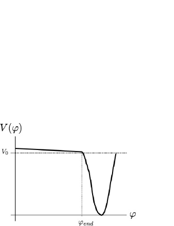
Figure 1: The prototypical inflaton potential. Achieving a flat potential which suddenly drops at $\varphi_{end}$ requires tuning the coefficients of a series of higher-dimensional operators.

This raises the question of whether inflation in our universe is the result of a “chance” tuning among couplings or of a deeper mechanism. Directly or indirectly, the answer can have observable ramifications. For example, the degree of tuning increases as the scale of inflation is lowered, so it is much more likely that an inflationary potential arises by chance for the case of high-scale inflation than for low-scale inflation. On the other hand, some models of fundamental physics produce unwanted particles (for example, late-decaying gravitinos Krauss1983556 ), defects, or other inhomogeneities at relatively low scales, features that can be erased by low-scale inflation. An underlying mechanism for inflation might have less of a high-scale bias and make such models more plausible. Of course, a particular mechanism for inflation may give rise to new cosmological signatures.

Several broad mechanisms have been discussed in the literature. It seems natural to turn to symmetries in order to explain the special features of an inflationary potential, in particular the slow-roll region. Supersymmetric theories do often have “flat directions” in field space, but inflationary curvature breaks supersymmetry badly enough that it cannot by itself explain the flatness of the inflaton potential Copeland:1994vg ; Lyth:1998xn ; Randall:1997kx . Instead, in Natural Inflation Freese:1990rb this flatness is ensured by realizing the inflaton as a pseudo Nambu-Goldstone boson (PNGB), protected by the associated (approximate) shift-symmetry. But this still leaves the challenge of escaping from slow-roll to reheating. Hybrid Inflation Linde:1993cn provides an elegant answer to the sudden change in shape of the potential. The central insight is that with multiple fields, the path in field space can take sudden turns in response to even a gently varying potential landscape. The sudden change in potential of Fig. 1 can then be traced out along such a “bent” path.

Let us examine hybrid inflation more carefully, along the lines of Ref. ArkaniHamed:2003mz . The prototypical model of hybrid inflation has two fields, the inflaton field $\Pi(x)$ and a “waterfall” field $\omega(x)$, with potential (in Einstein frame),

$$V = \frac{m_{\Pi}^{2}}{2}\Pi^{2}+g_{1}\Pi^{2}\omega^{2}+g_{2}(\omega^{2}-\omega_{1}^{2})^{2}$$ (1)

$$= \frac{m_{\Pi}^{2}}{2}\Pi^{2}+(g_{1}\Pi^{2}-2g_{2}\omega_{1}^{2})\omega^{2}+g_{2}\omega^{4}+g_{2}\omega_{1}^{4},$$

where $\omega_{1}$ sets the true vacuum, $\omega=\omega_{1},\Pi=0$ at zero vacuum energy. However if one starts cosmic evolution at sufficiently large $\Pi=\Pi_{0}\neq 0$, then the second line shows that one can effectively have a $\Pi$-dependent mass-squared for $\omega$, which stabilizes $\omega=0$. Plugging this back into $V$, gives an effective potential for just $\Pi$,

$$V_{eff}(\Pi)=\frac{m_{\Pi}^{2}}{2}\Pi^{2}+g_{2}\omega_{1}^{4}.$$ (2)

For small $m_{\Pi}^{2}$, $\Pi$ rolls slowly to smaller values and results in inflation, with Hubble constant given by $H^{2}M_{Pl}^{2}\simeq g_{2}\omega_{1}^{4}$. While $V_{eff}$ itself does not describe how inflation ends, it does end suddenly when the $\Pi$-dependent mass term for $\omega$ turns tachyonic, and $\omega$ is destabilized from the origin towards the true vacuum at $\omega_{1}$.

It has been suggested that the smallness of $m_{\Pi}^{2}$ can be explained by realizing $\Pi$ as a PNGB ArkaniHamed:2003mz ; Kaplan:2003aj . This is an attractive strategy, using approximate shift symmetry to do what it does best, protecting the flatness of the inflaton potential, while using the waterfall mechanism to do what it does best, namely ending inflation. But at the quantum level we must check that the levels of shift-symmetry breaking by $m_{\Pi}^{2}$ and $g_{1}$ are naturally compatible. Indeed, without further structure they are not, as can be seen by studying the one-loop renormalization of $m_{\Pi}^{2}$ by $g_{1}$,

$$\Delta_{\omega-loop}m_{\Pi}^{2}\sim\frac{g_{1}\Lambda_{UV}^{2}}{16\pi^{2}},$$ (3)

where $\Lambda_{UV}$ is the cutoff of this effective field theory.

At the start of inflation we need positive $\Pi$-dependent mass-squared for $\omega$,

$$g_{1}\Pi_{0}^{2}>2g_{2}\omega_{1}^{2}\simeq\frac{H^{2}M_{Pl}^{2}}{\omega_{1}^{2}},$$ (4)

which then implies,

$$\Delta_{\omega-loop}m_{\Pi}^{2}\gtrsim\frac{M_{Pl}^{2}\Lambda_{UV}^{2}}{16\pi^{2}\omega_{1}^{2}\Pi_{0}^{2}}H^{2},$$ (5)

Technical naturalness requires $m_{\Pi}^{2}\gtrsim\Delta_{\omega-loop}m_{\Pi}^{2}$, while the slow-roll conditions require $m_{\Pi}^{2}\ll H^{2}$, from which we conclude that

$$\frac{M_{Pl}\Lambda_{UV}}{\omega_{1}\Pi_{0}}<1.$$ (6)

But this is only possible for fields larger than the cutoff or the Planck scale. Moving away from this dangerous regime for effective field theory, the model rapidly becomes fine-tuned.

Refs. ArkaniHamed:2003mz ; Kaplan:2003aj describe new physics that can cut off the quadratic divergence above and thereby resolve the fine-tuning problem, either based on extra dimensions, supersymmetry or the Little Higgs mechanism. In the present paper we describe a new approach that can be thought of as using compositeness of the inflaton and waterfall fields in order to cut off UV sensitivity. If this is the case, one would expect the compositeness scale to cut off quantum loops involving the light composite fields. But this would appear to only reinterpret $\Lambda_{UV}$ as a physical compositeness scale, without altering the conclusion that fields must take on Planckian values in order to preserve naturalness. We therefore take $\Pi$ and $\omega$ to be composites of two separate sectors, with different compositeness scales, $\Lambda_{\Pi}$ and $\Lambda_{\omega}$ respectively. The $\omega$-loop would then be cut off by $\Lambda_{UV}\equiv\Lambda_{\omega}$. Naturalness can then be satisfied with sub-Planckian and sub-cutoff fields if

$$\Lambda_{\Pi}\gg\Lambda_{\omega}.$$ (7)

In particular, Eq. (6) can be satisfied by $\Lambda_{UV}\equiv\Lambda_{\omega}\ll\Pi_{0}$.

A theory based on compositeness would ordinarily run into the requirement of understanding the underlying strong coupling dynamics. However, exploiting AdS/CFT duality Maldacena:1997re ; Gubser:1998bc ; Aharony:1999ti ; Witten:1998qj we can present the same ideas in terms of weakly-coupled higher-dimensional (minimally 5D) effective field theory within warped throats, one for each of the two composite sectors. Here we proceed minimally within 5D effective field theory based on the Randall-Sundrum I (RS1) model Randall:1999ee . The connections between such throats and 4D CFT’s were developed in Ref’s  Verlinde:1999fy ; maldacenaunpub ; wittenITP ; Verlinde:1999xm ; Gubser:1999vj ; ArkaniHamed:2000ds ; Rattazzi:2000hs ; PerezVictoria:2001pa The fields $\Pi$ and $\omega$ are then realized as light moduli within each of the two throats. It is attractive to realize $\Pi$ as a composite PNGB for the reasons described above. The AdS/CFT dual of this is that $\Pi$ is the fifth component of a 5D gauge field Contino:2003ve . In the next section we will argue for identifying the waterfall field $\omega$ with the “radion” modulus of an RS1 throat.

With such an identification, the relaxation of $\omega$ from a metastable VEV to its true-vacuum VEV corresponds to the motion of the IR boundary of the RS1 throat. In this sense it superficially resembles the approach of Brane Inflation Dvali:1998pa ; Kachru:2003sx . The difference is that in Brane Inflation it is the inflaton that is realized as a mobile brane while here it is the waterfall field that is a mobile “brane”. The usual Brane Inflation strategy is to geometrically realize inflaton shift-symmetry as approximate brane translation invariance when the inflaton brane is far from other higher-dimensional objects. However, this symmetry is typically spoiled once the higher dimensions are compactified down to 4D, and gravitational backreaction taken into account Kachru:2003sx . By comparison, shift symmetry in extra-dimensional components of gauge fields is quite robust.

There is an important difference between the effective potential of our model and the model of Eq. (1), illustrated in Fig. 2. Here we plot both potentials as a function of the waterfall field for the inflationary value of the inflaton. While in the model of elementary fields - see Fig. 2(a) - the inflationary VEV of $\omega$ is the true minimum of the potential at $\Pi_{0}$, in our model - see Fig. 2(b) - the inflationary VEV is a metastable local minimum. In both cases as the inflaton rolls, the picture changes and the inflationary $\omega$ VEV is destabilized classically towards the true vacuum. But in our model, there is always the alternate possibility of quantum tunnelling to the true vacuum earlier. This would be a phenomenological disaster if tunneling dominated the end of inflation, but may provide an interesting phenomenology if it is subdominant Guth:1980zm ; Liddle:1991tr . In this paper, we will study the issue of tunneling just enough to choose a region of parameter space where it is completely suppressed in our universe. But in future work we will return to study its phenomenological prospects.

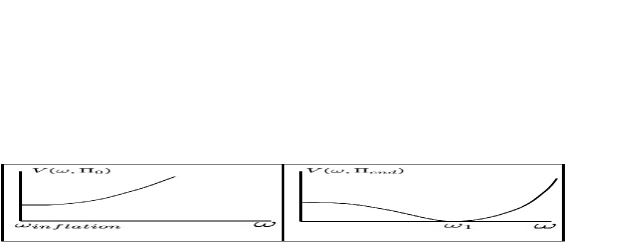
(a)  Standard Hybrid Inflation

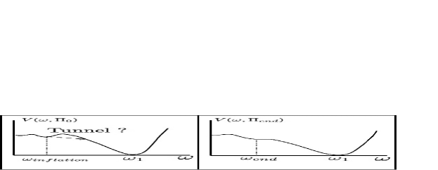
(b)  Warped Hybrid Inflation

Figure 2: ‘Animations’ of standard Hybrid Inflation - as in Eq. (1) - and Warped Hybrid Inflation. Note that in the the warped case, inflation takes place while the waterfall is at a metastable minimum.

While we present our model within 5D effective field theory, the ingredients of the model seem to be compatible with string theory, as it is currently understood, and we hope that our work will help identify inflating string theories within the “landscape” Susskind:2003kw . This raises the question of the role of supersymmetry. In our model, supersymmetry plays almost no role, although it is compatible with high-scale supersymmetry. The possible auxiliary role will be commented on in the last section. In this paper, we will focus on arriving at a natural theory of high-scale inflation, because this is the easiest target. However, our goals are broader and include understanding whether low-scale inflation can naturally occur. We expect that supersymmetry plays a more important role here. But we will leave such an investigation for future work.

The paper is organized as follows. In Section II, we will motivate in the language of strongly-coupled compositeness, the strategy behind our model, and then translate the key ingredients into the language of weakly-coupled warped 5D effective field theory using the AdS/CFT duality. In Section III we present our two-throat model, their light moduli, and their couplings. Because $\Lambda_{\Pi}$ need not be too small we will realize the dual inflaton throat as negligibly warped. In Section IV we derive the low-energy effective $\Pi-\omega$ theory and a variety of constraints that simplify our analysis and ensure a generalized hybrid inflation structure for the effective potential. In Section V we discuss quantum tunneling from the metastable to stable $\omega$ vacuum. In Section VI we integrate out $\omega$ during inflation and arrive at an effective theory for just $\Pi$, and check the slow-roll conditions. In Section VII we estimate the leading quantum corrections to the 5D action. In Section VIII we present an illustrative set of parameters, which are not fine-tuned, in which successful inflation takes place. In Section IX we discuss our results.

II Compositeness Strategy

Let us begin by thinking of our two fields as composites of different strongly-interacting sectors in purely 4D spacetime. We ask how a “waterfall” cross-coupling of $\Pi$ to $\omega$ can arise. In general cross-couplings arise by multiplying composite operators (which interpolate the composites) from each of the two sectors within the Planck-scale Lagrangian,

$${\cal L}(M_{Pl})\ni\frac{{\cal O}_{\Pi}(x){\cal O}_{\omega}(x)}{M_{Pl}^{d_{\Pi}+d_{\omega}-4}},$$ (8)

where the operators have high-energy scaling dimensions $d_{\Pi}$ and $d_{\omega}$. Below $\Lambda_{\Pi}$, ${\cal O}_{\Pi}$ “hadronizes” into some function of the light composite $\Pi$,

$${\cal L}_{eff}(\Lambda_{\Pi})\ni\frac{\Lambda_{\Pi}^{d_{\Pi}}f(\Pi/\Lambda_{\Pi}){\cal O}_{\omega}(x)}{M_{Pl}^{d_{\Pi}+d_{\omega}-4}}.$$ (9)

The generalization of a $\Pi$-dependent “mass term” for $\omega$, is a $\Pi$-dependent coefficient of a relevant operator in the $\omega$-sector, that is,

$$d_{\omega}<4.$$ (10)

Below $\Lambda_{\omega}$ this sector also hadronizes and we obtain

$${\cal L}_{eff}(\Lambda_{\omega})\ni\frac{\Lambda_{\Pi}^{d_{\Pi}}f(\Pi/\Lambda_{\Pi})\Lambda_{\omega}^{d_{\omega}}g(\omega/\Lambda_{\omega})}{M_{Pl}^{d_{\Pi}+d_{\omega}-4}}.$$ (11)

However, there is a problem with the general structure of such a cross-coupling for the purpose of inflation, namely $g(\omega_{inflation}/\Lambda_{\omega})$ has no particular reason to be small, which in turn leads to an inflaton mass contribution,

$$\Delta m_{\Pi}^{2}\sim\frac{\Lambda_{\Pi}^{d_{\Pi}-2}\Lambda_{\omega}^{d_{\omega}}}{M_{Pl}^{d_{\Pi}+d_{\omega}-4}}.$$ (12)

We can estimate this by noting that we want different values of the cross-coupling (for differing values of $\Pi$) to be responsible for the drop in potential energy density, from inflation at $\sim H^{2}M_{Pl}^{2}$, to the true vacuum at zero. Without any special structure,

$$\frac{\Lambda_{\Pi}^{d_{\Pi}}\Lambda_{\omega}^{d_{\omega}}}{M_{Pl}^{d_{\Pi}+d_{\omega}-4}}\gtrsim H^{2}M_{Pl}^{2}.$$ (13)

We therefore find,

$$\Delta m_{\Pi}^{2}\gtrsim H^{2}\frac{M_{Pl}^{2}}{\Lambda_{\Pi}^{2}},$$ (14)

which violates slow-roll (since $\Lambda_{\Pi}\lesssim M_{Pl}$), unless fine-tuned away. This should be compared with the model of Eq. (1), in which the cross-coupling itself (at $\Pi_{0}$) drives $\omega\rightarrow 0$, which in turn suppresses the $\Pi$ mass contribution from this coupling.

But there is a special kind of strongly-interacting composite theory that shares this feature of the elementary model, namely a conformal field theory (CFT) which undergoes spontaneous breaking of conformal invariance. It must give rise to a (composite) Nambu-Goldstone boson, which we will identify with $\omega$. In such a scale-invariant dynamics, there is no independent compositeness scale $\Lambda_{\omega}$, but instead

$$\Lambda_{\omega}\equiv\langle\omega\rangle.$$ (15)

The IR cross-coupling then takes the form

$${\cal L}_{eff}(\Lambda_{\omega})\ni\frac{\Lambda_{\Pi}^{d_{\Pi}}f(\Pi/\Lambda_{\Pi})\omega^{d_{\omega}}}{M_{Pl}^{d_{\Pi}+d_{\omega}-4}}.$$ (16)

As in the elementary model, this potential itself can drive $\omega$ to small values during inflation and large values at reheating, but unlike the elementary model a small (but non-zero) $\omega_{inflation}$ also acts as a low cutoff on the $\omega$ loops renormalizing the inflaton mass.

A second issue is that given Eq. (10), we must ask why our Lagrangian does not naturally contain

$${\cal L}(M_{Pl})\ni M_{Pl}^{4-d_{\omega}}{\cal O}_{\omega},$$ (17)

which would overwhelm all other dynamics with its Planckian mass scale. In the model of Eq. (1), this is the question of why we did not write a mass term $M_{Pl}^{2}\omega^{2}$ given we have $\Pi^{2}\omega^{2}$. But in the case of compositeness such a relevant coupling can be forbidden if ${\cal O}_{\Pi}$ and ${\cal O}_{\omega}$ transform under a high-energy symmetry, such that only their product is invariant, for example if they were each odd under a $\mathbb{Z}_{2}$-symmetry. This symmetry can then be broken at the compositeness scales of each sector, in particular by $\langle\omega\rangle$ in the $\omega$ sector.

Now let us use the AdS/CFT correspondence to translate the above elements to weakly-coupled but higher-dimensional (minimally 5D) effective field theory within two warped throats, one for each of the two composite sectors. The fields $\Pi$ and $\omega$ are then realized as light moduli within each of these throats. It is attractive to realize $\Pi$ as a composite PNGB for the reasons described above. The AdS/CFT dual of this is to that $\Pi$ is the fifth component of a 5D gauge field. Taking $\omega$ to be the “radion” modulus of an RS1 throat gives the minimal dual incarnation of a PNGB of spontaneous conformal symmetry breaking ArkaniHamed:2000ds ; Rattazzi:2000hs . The dual of the operators ${\cal O}$ are then scalar fields propagating within each throat, which can be coupled on their shared UV brane. The relevance of the operator ${\cal O}_{\omega}$ translates into it being an AdS tachyon in the RS1 throat. The danger this poses to the throat stability then requires assigning it symmetry quantum numbers, minimally a discrete $Z_{2}$ symmetry. This summarizes the strategy underlying what follows.

III The Model

The 5D model consists of an extra dimensional interval with two boundaries and one intermediate 3-brane which splits spacetime into two regions, as shown in Fig. 3. One region we call the “waterfall throat”, and it is a highly warped RS1-like throat with its light radion ultimately playing the role of the waterfall field of hybrid inflation. The intermediate brane acts as the UV brane for this throat. The second region is taken to be only mildly warped, although for convenience we will refer to it as the “inflaton throat.” In it the inflaton of hybrid inflation is realized as the $A_{5}$ component of a 5D gauge field. With the exception of the metric of 5D General Relativity, each region has separate field content. Nevertheless, non-gravitational fields can meet and interact at the intermediate UV brane. In particular, such a cross-coupling between throats will result in the coupling of inflaton and waterfall fields that plays a central role in hybrid inflation.

Figure 3: Schematic for the bulk symmetries and brane localized symmetry breakings of the two throat system. The $U(1)$ is gauged and its fifth component gives us a PNGB inflaton. The parities $\mathbb{Z}_{2}$ and $\mathbb{Z}^{\prime}_{2}$ are matter symmetries that constrain the symmetry breaking patterns in the waterfall throat.

The 5D action of the full theory takes the form

$$S=S_{infl}+S_{water}+S_{cross},$$ (18)

where the first two terms on the right describe couplings in each of the two throats separately and the last term describes the origins of the inflaton-waterfall cross-coupling and related physics; see Figure 3 for a schematic of the action in Eq. (18). This division is also convenient because the first two terms correspond to rather standard modules in the literature Hosotani:1983xw ; Hosotani:1988bm ; Hatanaka:1998yp ; Antoniadis:2001cv ; Cheng:2002iz ; vonGersdorff:2002as and Randall:1999ee $+$ GW . (See Reference Sundrum:2005jf for a review of both modules.) In the next three subsections we will flesh out each of these terms in the action. In this section we focus on the physics that we actually want. Of course it is important to consider corrections that might destabilize the desired inflationary outcome, and we do this in Section VII.

III.1 The Inflaton Throat

The inflaton throat is a finite interval whose size we denote by $\pi L$. We realize this interval as an $S_{1}/\mathbb{Z}_{2}$ orbifold and we identify the orbifold fixed points at $y=0~{}$and$~{}\pi L$. This will be a convenient way of assigning boundary conditions for fields. The bulk fields of the throat consist of a $U(1)$ gauge field $A_{M}$, a heavy charged scalar $\Sigma$, 5D gravity, and neutral scalar fields that stabilize the throat geometry. On top of all these fields the throat will also contain very heavy fields associated with the UV completion of the non-renormalizable 5D effective field theory. However, the physics we will rely on will require propagation across the entire throat and will therefore be insensitive to the very short range effects of the UV completion. In particular, the purpose of this sector is to realize a 4D inflaton as the $A_{5}$ component of a gauge field ArkaniHamed:2003mz ; Kaplan:2003aj .

The physics of the inflaton throat is given by:

$$S_{infl} =S_{U(1)}+S_{\Sigma}+S_{stab}+S_{gravity},$$ (19)

$$S_{U(1)} =-\frac{1}{4}\int d^{4}x\int dy\sqrt{G}G^{MN}G^{KL}F_{MK}F_{NL}$$

$$S_{\Sigma} =\int d^{4}x\int dy\sqrt{G}\left\{G^{MN}D_{M}\Sigma^{\dagger}D_{N}\Sigma-m_{\Sigma}^{2}|\Sigma|^{2}\right\}$$

The extra-dimensional geometry of the inflaton throat can be stabilized by the Goldberger-Wise (GW) mechanism GW . This is the content of $S_{stab}$. For simplicity we consider an inflaton throat which is very mildly warped. Stabilization energies can then be not much smaller than the compactification scale which we will take much higher than the scales relevant to inflation, so that the throat is essentially rigid on the scales of interest. That is we can simply take the 5D metric in this throat to be of the form

$$ds^{2}\approx g_{\mu\nu}(x)dx^{\mu}dx^{\nu}-dy^{2},$$ (20)

$g_{\mu\nu}(x)$ is the 4D zero-mode gravitational field. We will be more explicit about Goldberger-Wise stabilization dynamics in the waterfall throat where it plays a more important role.

We focus more carefully on the gauge sector. We assign orbifold parity to the gauge field in the following way: $P(y)=-y$, $P(A_{\mu})=-A_{\mu}$, $P(A_{5})=A_{5}$ and $\Sigma$ is assigned even parity. This parity assignment ensures the existence of an approximately massless zero mode for the fifth component of the gauge field: $A_{5}$. Indeed the rest of $A_{5}$ can be gauged away, so that $A_{5}$ can be taken to be $y$-independent. The remaining modes are all Kaluza-Klein (KK) modes and have masses at the compactification scale $\sim 1/L$. $\Sigma$ does not yield any light mode for large bulk mass. Gauge-invariantly the $A_{5}$ zero-mode corresponds to the Wilson loop around the compactification, $W(x^{\mu})\equiv\exp(ig_{5}\oint_{S_{1}}dyA_{5}(x^{\mu},y))$, which in the present gauge is $W(x)=e^{i2\pi Lg_{5}A_{5}(x)}$. We see that the zero mode is an angular variable, essentially a 4D pseudo-Nambu-Goldstone boson (PNGB). The corresponding “decay constant,” $f_{\pi}$, follows by going to the canonically normalized $\Pi(x)\equiv A_{5}(x)\sqrt{\pi L}$,

$$S_{U(1)}\xrightarrow[IR]{}S_{\Pi}=\int\sqrt{-g}\,d^{4}x\frac{g^{\mu\,\nu}\partial_{\mu}\Pi\partial_{\nu}\Pi}{2},$$ (21)

in terms of which the gauge-invariant observable is

$$W(x)\equiv e^{i\Pi(x)/f_{\pi}},$$ (22)

with

$$f_{\pi}=\frac{1}{2\,g_{5}\sqrt{\pi L}}.$$ (23)

The 5D non-locality of $\Pi$ protects its potential from short-range effects such as the physics of the UV completion. Instead its potential is determined by the lightest charged fields that can propagate around the compactification, in the present case the 1-loop propagation of $\Sigma$, in a constant $\Pi$ background (constant since we are only after the $\Pi$ effective potential) Hosotani:1983xw ; Hosotani:1988bm ; Hatanaka:1998yp ; Antoniadis:2001cv ; Cheng:2002iz ; vonGersdorff:2002as . For $m_{\Sigma}\pi L\gg 1$ this is

$$V_{\Sigma-loop}(\Pi)\sim-\frac{m_{\Sigma}^{2}}{8\pi^{4}L^{2}}e^{-2\pi Lm_{\Sigma}}\cos\left(\frac{\Pi}{f_{\pi}}\right).$$ (24)

The exponential suppression is the Yukawa suppression for the massive field to virtually propagate around the compactification and “measure” the Wilson loop $e^{i\Pi/f_{\pi}}$. We will see that this potential can dominate the slow-roll of the inflaton during inflation.

Brane-localized couplings, predominantly linear or “tadpole” couplings of $\Sigma$, could affect the effective potential for $\Pi$. They are allowed by the orbifold breaking of 5D gauge invariance and we will make use of such couplings in subsection III.3.

The various contributions to the 4D low-energy physics from this throat are then given by

$${\cal L}_{eff,infl}=\sqrt{g}\left\{M_{5}^{3}\pi L{\cal R}^{(4)}+g^{\mu\nu}\frac{\partial_{\mu}\Pi\partial_{\nu}\Pi}{2}-V_{\Sigma,\,loop}(\Pi)-\rm constant\right\},$$ (25)

where $g_{\mu\nu}(x)$ is the 4D gravity zero mode, ${\cal R}^{(4)}$ is its curvature, $M_{5}$ is the 5D Planck scale, and we do not specify the constant piece of the potential since brane tensions effectively act as “counterterms” that we can dial for it. (We allow ourselves one fine-tuning in the end, namely the 4D cosmological constant after reheating.)

III.2 The Waterfall Throat

The waterfall throat is a finite interval whose size we denote by $\pi r$. We realize this interval as an $S_{1}/\mathbb{Z}_{2}$ orbifold, distinct from that of the inflaton throat. We identify the orbifold fixed points at $y=0~{}$and$~{}\pi r$ as the UV and IR branes of this highly warped throat, where the UV brane is the intermediate brane of the entire set-up. Here, we limit ourselves to the physics relevant after reheating, in particular describing the true vacuum of the theory, deferring the subtler structure and fields needed for the inflationary era until subsection III.3. For our present purposes the waterfall throat is just a copy of the RS1 model (leaving out the Standard Model (SM) fields for simplicity), with minimal Goldberger-Wise stabilization GW . In particular, the field content we start with consists just of the 5D metric and the 5D Goldberger-Wise scalar $\Phi$. The structure of these is well-known and we will not write it out explicitly.

Instead we merely recall that the light 4D degrees of freedom consist of the 4D gravitational zero mode $g_{\mu\nu}(x)$, (the same as in subsection III.1) and the 4D radion of the waterfall throat, contributing to the 4D effective theory,

$${\cal L}_{eff,water}=\sqrt{g}\left\{\frac{M_{5}^{3}}{k}(1-\omega^{2}){\cal R}^{(4)}+\frac{6\,M_{5}^{3}}{k}g^{\mu\nu}\partial_{\mu}\omega\partial_{\nu}\omega+\lambda\frac{\omega^{4}}{4}-\kappa\frac{\omega^{4+\gamma}}{4+\gamma}-{\rm constant}\right\},$$ (26)

where the maximal warp factor $\omega(x)\equiv e^{-k\pi r(x)}$ is the convenient choice of radion field, $r(x)$ is the dynamical proper length of the throat, and $1/k$ is the radius of curvature of the approximately $AdS_{5}$ local bulk geometry,

$$ds^{2}\approx e^{-2ky}g_{\mu\nu}(x)dx^{\mu}dx^{\nu}-dy^{2}.$$ (27)

The $\kappa$ coupling is the leading effect of integrating out the 5D Goldberger-Wise scalar with $m_{\Phi}^{2}\equiv\gamma(4+\gamma)k^{2}$ and with brane-localized couplings $J_{IR}\Phi$ and $J_{UV}\Phi$:

$$\frac{\kappa}{4+\gamma}\sim\frac{J_{IR}J_{UV}}{k}.$$ (28)

The constant contribution is again not specified because the UV brane tension acts as a counterterm that allows us to choose it to cancel the cosmological constant after reheating. The $\lambda$ coupling arises when the IR boundary “tension” is not at the RS1 tuned value. We assume this more generic “de-tuned” choice of tension,

$$\frac{\lambda}{4}=T_{RS}-T.$$ (29)

The $\lambda,\kappa$ couplings (chosen positive) lead to a stabilizing potential for $\omega$ and hence a finite length of throat. This vacuum state will describe the vacuum of the theory after reheating. In the next subsection we will turn to the fields, symmetries and physics that put us in an inflationary state.

Again, we have left out the Standard Model fields for ease of explanation, but we note that the simplest possibility is to place the Standard Model on the IR brane of the waterfall throat. The radion, as the dual to the dilaton, couples to breaking of scale invariance, i.e. mass terms. If the visible sector contains a scalar $\phi_{vis}$ with mass $m_{vis}$ then the radion coupling to the visible sector is given by:

$${\cal L}_{\omega-vis}\approx\delta\omega\,m_{vis}^{2}\phi_{vis}^{2},$$ (30)

where $\delta\omega$ is the fluctuation of the radion field from its vev. The lesson here is that the radion will decay preferentially to the heaviest particle kinematically accessible. This might be a SM field, or more generally, a heavier field on the IR brane with appreciable couplings and decays to the SM.

III.3 The Inflaton-Waterfall Cross-Coupling

We now add two new bulk (orbifold-even) real scalars, $\chi_{i=1,2}$, to the warped waterfall throat (but not in the inflaton throat), which however have tachyonic masses,

$$S_{tachyons}=\int d^{4}x\int dy\sqrt{G}\,\frac{1}{2}\left\{G^{MN}\partial_{M}\chi_{i}\partial_{N}\chi_{i}-m_{i}^{2}\chi_{i}^{2}\right\},~{}~{}0>m_{i}^{2}\geq-4k^{2}.$$ (31)

While tachyons above the Breitenlohner-Freedman bound Breitenlohner:1982bm $m_{5}^{2}\geq-4k^{2}$ do not imply any instability in infinite $AdS_{5}$ spacetime, they are a potential source of instability for RS1. UV-brane localized tadpole (linear) couplings in the tachyon field will source growing profiles in the IR which can blow up before reaching the IR boundary. We therefore introduce two new discrete symmetries, $\mathbb{Z}_{2},\mathbb{Z}_{2}^{\prime}$, to control tadpole couplings. We take $\chi_{1}$ to be odd under $\mathbb{Z}_{2}$ and even under $\mathbb{Z}_{2}^{\prime}$, and $\chi_{2}$ to be odd under $\mathbb{Z}_{2}^{\prime}$ and even under $\mathbb{Z}_{2}$. We will also assign $\Sigma$, from the inflaton throat, to be odd under $\mathbb{Z}_{2}^{\prime}$ and even under $\mathbb{Z}_{2}$. We will take these symmetries to be fully broken on the boundaries of the inflaton and waterfall throats. We only need the protection of these symmetries in the bulk and on the UV (middle) brane; $\mathbb{Z}_{2}^{\prime}$ is taken to be exact in these regions, while $\mathbb{Z}_{2}$ is slightly broken.

Finally, we add a set of localized couplings on all three branes and boundaries of our entire set-up. Denoting the brane induced 4-metric by $G_{\mu\nu}^{ind}$,

$$S_{infl\,bdry} = \int d^{4}x\sqrt{G_{ind}}\,\left.\left(\vphantom{\sqrt{G_{ind}}}J_{1}\Sigma+J_{1}^{\dagger}\Sigma^{\dagger}\right)\right|_{boundary}$$

$$S_{water\,bdry} = \int d^{4}x\left.\sqrt{G_{ind}}\left(\vphantom{\sqrt{G_{ind}}}J_{4}\chi_{2}-J_{5}\chi_{1}-\mu_{1}\,\chi_{1}^{2}-\mu_{2}\,\chi_{2}^{2}\right)\right|_{boundary}$$

$$S_{mid\,brane} = \int d^{4}x\sqrt{G_{ind}}\left\{\vphantom{\sqrt{G_{ind}}}j_{3}\chi_{1}+\left.(J_{2}\,\Sigma+J_{2}^{\dagger}\,\Sigma^{\dagger})\chi_{2}-\mu_{1}^{(\textrm{UV)}}\chi_{1}^{2}-\mu_{2}^{(\textrm{UV})}\chi_{2}^{2}\right\}\right|_{brane},$$

where “$|_{brane,\,boundary}$” just means the evaluation of the bulk field at the $y$-location of the brane or boundary in question. The $J,j$’s and $\mu$’s are constants.

We denote the $\chi_{1}$ source on the middle brane with a small $j$ to indicate that it is taken to be much smaller than the fundamental scale, whereas the capital $J$ coefficients are supposed to be only modestly smaller than the fundamental scale. The smallness of $j_{3}$ is technically natural, corresponding to a small breaking of the $\mathbb{Z}_{2}$ symmetry on this brane. The $J_{2}$ coupling is linear in each of $\Sigma$ and $\chi_{2}$, a kind of brane-localized mixing mass term, coupling a waterfall throat field to an inflaton throat field at their shared border. Note that this coupling is fully symmetric, but separate tadpole couplings in either $\Sigma$ or $\chi_{2}$ are forbidden on the middle brane.

Assembling the above pieces defines

$$S_{cross}\equiv S_{tachyons}+S_{infl\,bdry}+S_{water\,bdry}+S_{mid\,brane}.$$ (33)

Let us see what leading corrections this makes to our 4D effective theory. We will choose the brane/boundary tachyon masses, $\mu$, to all be positive and order $k$ so that neither tachyon field leads to any 4D light or 4D tachyonic modes in the KK decomposition. We can therefore completely integrate out $\chi_{i}$ in arriving at the 4D effective theory Davoudiasl:2005uu . We begin by integrating out the $\chi_{1}$ tachyon, sourced by $j_{3},J_{5}$, which then corrects the radion potential. We can do the Feynman diagrams shown in Fig. 4 in mixed position-momentum space, where the 4D momentum is zero since we are implicitly computing an effective potential correction in the radion background (that is, an $x$-independent IR brane position). Using the RS scalar field propagator Contino:2003ve with brane masses $\sim k$, we find

$$\Delta V_{eff}(\Pi,\omega)=-\frac{j_{3}J_{5}}{k}\omega^{2+\alpha_{1}}.$$ (34)

Figure 4: Generic mixed position-momentum space Feynman diagram giving rise to the potential in Eq. (34). The index $i$ runs over the bulk fields: $\chi_{1}$, $\chi_{2}$ and $\Phi$. The functions $G_{i}$ are the mixed position-momentum space propagators appropriate to the bulk fields and the sources $\mathcal{J}_{i,UV}$ and $\mathcal{J}_{i,IR}$ are the tadpoles: $j_{3}$, $J_{2}$, $J_{UV}$ and $J_{5}$, $J_{4}$, $J_{IR}$ respectively.

Similarly, we can do the diagram of Fig. 5 by integrating out $\chi_{2}$ and $\Sigma$. We get the product of their propagators $\times$ sources,

$$\Delta V_{eff}(\Pi,\omega)=-\frac{J_{1}J_{2}J_{4}}{m_{\Sigma}k}e^{-m_{\Sigma}\pi L}\cos\left(\frac{\Pi}{2f_{\pi}}+\sigma\right)\,\omega^{2+\alpha_{2}},$$ (35)

where $\sigma=\arg(J_{1}\,J_{2}).$ The $\Pi$-dependence arises because we are computing the $\Sigma$ propagator in a constant $A_{5}$ background, in order to determined the latter’s effective potential. We therefore end up with the parallel transport phase factor across the inflaton throat for $\Sigma$, plus that for $\Sigma^{\dagger}$. The factor of $1/2$ in the cosine relative to Eq. (24) arises because we are only propagating one-way across the inflaton throat rather than round-trip.

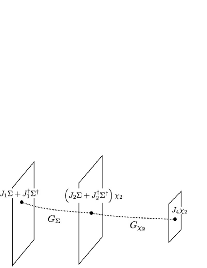
Figure 5: Feynman diagram giving rise to the ‘waterfall’ coupling in Eq. (35). The 4D coupling is naturally small because it arises from dynamics which are non-local in the extra dimension.

Note that the fundamental scale near the IR boundary of the waterfall throat is warped down $\propto\langle\omega\rangle$, as is standard in RS1. That translates into maximal energy densities localized near the IR boundary that scale $\propto\langle\omega\rangle^{4}$. Given that the radion itself, $\omega(x)$, is localized near the IR boundary, we see that the tachyonic nature of the $m_{\chi}^{2}<0,\alpha<2$, translates into potential energy densities that drop more slowly with small $\langle\omega\rangle$ (which will be the regime of interest). If all other factors were near the fundamental scale, the potential energy densities would violate the maximal energy density bound of 5D effective field theory. This reflects the general danger of instability that tachyonic scalars pose to RS1. This is precisely where the protective symmetries $\mathbb{Z}_{2},\mathbb{Z}_{2}^{\prime}$ come in. The small breaking of $\mathbb{Z}_{2}$ on the middle brane translates into a small $j_{3}$ which can suppress the first potential energy density in Eq. (34). The exact $\mathbb{Z}_{2}^{\prime}$ on the middle brane requires the linear $\chi_{2}$ dependence to multiply $\Sigma$. This in turn requires a $\Sigma$ propagation across the inflaton throat which is Yukawa-suppressed by $e^{-\pi Lm_{\Sigma}}$. We will ensure that we choose parameters such that these suppression factors keep us within effective field theory control.

IV The 4D $\Pi-\omega$ Effective Field Theory

Below the compactification scales of the two throats, there are just three 4D effective fields, $\Pi(x),\omega(x)$, and the zero mode metric $g_{\mu\nu}(x)$. Adding the contributions from Eqs. (24, 25, 34, 35 and 40) the 4D effective theory is given by

$${\cal L}_{eff} = \sqrt{g}\left\{g^{\mu\nu}\frac{\partial_{\mu}\Pi\partial_{\nu}\Pi}{2}+\frac{6\,M_{5}^{3}}{k}g^{\mu\nu}\partial_{\mu}\omega\partial_{\nu}\omega+\left(\frac{M_{5}^{3}}{k}(1-\omega^{2})+M_{5}^{3}\pi L\right){\cal R}^{(4)}\right.$$

$$- \left.\vphantom{g^{\mu\nu}\frac{\partial_{\mu}\Pi\partial_{\nu}\Pi}{2}}V_{eff}(\omega,\Pi)\right\}\,,$$

$$V_{eff}(\omega,\Pi) = -\frac{j_{3}J_{5}}{k}\omega^{2+\alpha_{1}}-\frac{J_{1}J_{2}J_{4}}{m_{\Sigma}k}e^{-m_{\Sigma}\pi L}\cos\left(\frac{\Pi}{2f_{\pi}}+\sigma\right)\omega^{2+\alpha_{2}}-\frac{\lambda}{4}\omega^{4}+\kappa\frac{\omega^{4+\gamma}}{4+\gamma}$$ (36)

$$- \frac{m^{2}_{\Sigma}}{8\pi^{4}L^{2}}e^{-2m_{\Sigma}\pi L}\cos\frac{\Pi}{f_{\pi}}+{\rm constant}.$$

The exponents are ordered as

$$0<\alpha_{1}<\alpha_{2}<2<2+\gamma$$ (37)

by our choice of bulk scalar masses in the waterfall throat.

Although $\omega$ is a dynamical variable we will always remain in a regime where $\omega\ll 1$. Therefore the 4D effective Planck scale is simply given by:

$$M_{Pl}^{2}\approx M_{5}^{3}(\pi L+1/k).$$ (38)

It is also convenient in what follows to trade other fundamental parameters of our model appearing above for new constant parameters, $\delta,\omega_{0},\omega_{1},v_{0},V_{0}$, implicitly defined by re-expressing the effective Lagrangian,

$${\cal L}_{eff} \approx \sqrt{g}\left\{g^{\mu\nu}\frac{\partial_{\mu}\Pi\partial_{\nu}\Pi}{2}+\frac{6\,M_{5}^{3}}{k}g^{\mu\nu}\partial_{\mu}\omega\partial_{\nu}\omega-\frac{M_{5}^{3}}{k}\omega^{2}{\cal R}^{(4)}+\frac{M_{Pl}^{2}}{2}{\cal R}^{(4)}\right.$$

$$- \left.\vphantom{\left\{g^{\mu\nu}\frac{\partial_{\mu}\Pi\partial_{\nu}\Pi}{2}\right.}V_{eff}(\omega,\Pi)\right\},$$

$$V_{eff}(\omega,\Pi) = -\frac{\delta\omega_{0}^{2-\alpha_{1}}}{2+\alpha_{1}}\omega^{2+\alpha_{1}}-\frac{\delta\omega_{0}^{2-\alpha_{2}}}{2+\alpha_{2}}\cos\left(\frac{\Pi}{2f_{\pi}}+\sigma\right)\omega^{2+\alpha_{2}}-\kappa\frac{\omega_{1}^{\gamma}}{4}\omega^{4}+\kappa\frac{\omega^{4+\gamma}}{4+\gamma}+$$ (39)

$$- v_{0}\cos\frac{\Pi}{f_{\pi}}+V_{0}.$$

It is also worthwhile summarizing here the constraints on field space. The angular nature of $\Pi$ means that without loss of generality, $0\leq\Pi(x)\leq 4\pi f_{\pi}$, and the warp factor nature of $\omega$ means that $0\leq\omega(x)\leq 1$.

We have chosen the above parametrization in anticipation of inflating at a metastable vacuum - $\omega_{inflation}\simeq\omega_{0}$ - and then rolling to reheat at the global minimum at $\omega_{reheat}\simeq\omega_{1}>\omega_{0}$. We must ensure that while $\omega\sim\omega_{0}$, $\Pi$ is rolling slowly toward $0$ under the influence of the effective potential, resulting in cosmic inflation. We will eventually choose a region of parameter space where the $v_{0}$ coupling dominates the slow-roll of $\Pi$. Taking $\sigma\sim\pi/2$, the potential is metastable in $\omega\sim\omega_{0}$ for $\Pi\sim\pi f_{\pi}$ and becomes unstable with $\omega$ rapidly rolling to $\omega_{1}$ for sufficiently small $\Pi$, resulting in reheating. This is the hybrid inflation mechanism we intend to pursue below in our model. A schematic diagram of the potential as well as the path taken in field space is given in Fig. 6.

In the remainder of this section, we study the classical waterfall field dynamics assuming that the inflaton $\Pi$ is indeed evolving very slowly. We study the inflationary regime where $\cos\left(\frac{\Pi}{2f_{\pi}}+\sigma\right)\sim-1$, and then the regime after reheating, where $\cos\left(\frac{\Pi}{2f_{\pi}}+\sigma\right)\sim 1$. This will allow us to pin down some of the constraints on our parameters. In the next section we consider the quantum subtlety of $\omega$ being able to tunnel from $\omega_{0}$ to $\omega_{1}$ even before it can classically roll there (again indicated in Fig. 6). In Section VI.2, we ensure that the effective potential for $\Pi$ does indeed satisfy the constraints for slow-roll inflation.

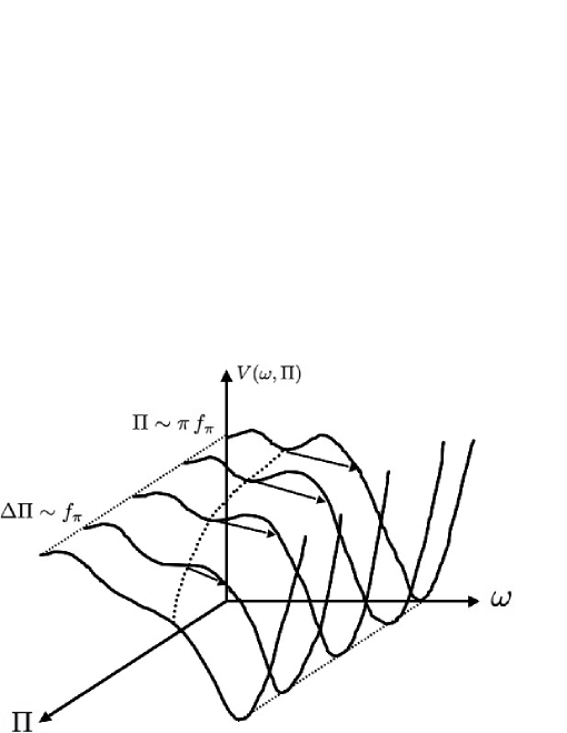
Figure 6: Schematic of the two-field potential - not to scale. Both fields move along classical trajectories determined by Eq. (IV) as in the dotted path. However, as indicated by the arrows in the diagram, $\omega$ can tunnel through a steadily decreasing barrier and then roll to the global minimum thus ending inflation early in a portion of the universe.

IV.1 The Effective Waterfall Potential for Fixed $\Pi$

During inflation we approximate $\cos\left(\frac{\Pi}{2f_{\pi}}+\sigma\right)\sim-1$, with $\sigma\sim\pi/2$. Furthermore, if successfully inflating, the 4D Ricci scalar is well approximated by $\mathcal{R}^{(4)}=12\,H^{2}$ which contributes to the $\omega$ mass through the $\mathcal{R}^{(4)}$ coupling in Eq. (IV). Thus, we consider the following effective potential for the waterfall; see Fig. 7 for a schematic of the waterfall potential during inflation:

$$V_{eff}(\omega)=12\,H^{2}\frac{M_{5}^{3}}{k}\omega^{2}-\frac{\delta\omega_{0}^{2-\alpha_{1}}}{2+\alpha_{1}}\omega^{2+\alpha_{1}}+\frac{\delta\omega_{0}^{2-\alpha_{2}}}{2+\alpha_{2}}\omega^{2+\alpha_{2}}-\kappa\frac{\omega_{1}^{\gamma}}{4}\omega^{4}+\kappa\frac{\omega^{4+\gamma}}{4+\gamma}+V_{0}.$$ (40)

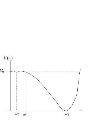
Figure 7: Schematic of the waterfall potential during inflation - not to scale. The inflaton is near $\pi f_{\pi}$ with $\sigma\sim\pi/2$, so that $\cos\left(\frac{\Pi}{2f_{\pi}}+\sigma\right)\approx-1$ and the waterfall sits in the metastable vacuum $\omega_{inflation}\approx\omega_{0}$ where the energy density is roughly $V_{0}$.

The simple operation of our model relies on the following constraints on the above potential:

• We have neglected the $\Pi$ potential energy density $v_{0}$ above by assuming parameters such that:

  $$v_{0}\ll V_{0}.$$ (41)

• We will arrange that during the evolution of the universe $\omega$ grows from $\sim\omega_{0}$ to $\sim\omega_{1}$. In this range it is important that the tachyon-induced potential energies never exceed the maximal energy densities allowed within 5D effective field theory near the waterfall IR boundary, as discussed at the end of subsection III.3. Even more strongly, we wish to stay below the energies at which the KK modes can be excited, so that we always are within 4D effective field theory. Since the KK masses of the warped throat are of order $k\omega$, this is satisfied if our physical radion mass is smaller than $(k\omega)^{2}$. We will arrange this by choosing:

  $$\delta\ll 12\,\pi^{2}\,M_{5}^{3}\,k.$$ (42)

• The second and third terms create a local minimum at $\omega_{0}$ as long as the effects of the first, fourth and fifth terms are negligible when $\omega\sim\omega_{0}$. This is satisfied if:

  $$12\frac{M_{5}^{3}}{k}H^{2}\ll\delta\omega_{0}^{2},$$ (43)

  $$\kappa\omega_{1}^{\gamma}\ll\delta.$$ (44)

• The fourth and fifth terms produce a global minimum at $\omega_{1}$ if we can neglect the first, second and third terms for $\omega\sim\omega_{1}$. We want the ordering of minima to satisfy

  $$\omega_{1}\gg\omega_{0}.$$ (45)

  Then the first three terms can be neglected for $\omega\sim\omega_{1}$ if

  $$12\frac{M_{5}^{3}}{k}H^{2}\ll\kappa\omega_{1}^{2+\gamma},$$ (46)

  $$\delta\omega_{0}^{2-\alpha_{2}}\ll\kappa\omega_{1}^{2+\gamma-\alpha_{2}}.$$ (47)

At late times, $\Pi$ slow-rolls to smaller values and the local minimum in the $\omega$ direction moves from $\omega_{0}$ to larger values, and then eventually disappears altogether. At this point, $\omega$ rolls to the global $\omega_{1}$ minimum, corresponding to reheating.

• The energy density at the global minimum $\omega_{1}$ is dominated by the last three terms. The vacuum energy here must vanish, requiring us to tune,

  $$V_{0}\approx\kappa\frac{\gamma\omega_{1}^{4+\gamma}}{4(4+\gamma)},$$ (48)

  This is the usual (fine-)tuning of the 4D cosmological constant of our universe to zero.

• Given our earlier choices, $V_{0}$ dominates over all the other terms in Eq. (40) during inflation, when $\omega\simeq\omega_{0}$. Therefore, the inflationary Hubble constant is given by:

  $$H^{2}_{inflation}\approx\kappa\frac{\gamma\omega_{1}^{4+\gamma}}{12(4+\gamma)M_{Pl}^{2}}.$$ (49)

• We leave the details of reheating after inflation to future work, but it is possible to estimate the reheat temperature in two simple cases.

  Instantaneous Decay

  If the waterfall were to decay instantaneously into relativistic particle species, thereby converting all of the inflationary energy density into radiation, one can estimate the reheat temperature:

  $$T_{instantaneous}^{4}\approx V_{0}\approx\kappa\omega_{1}^{4+\gamma}$$

  $$T_{instantaneous}\approx\kappa^{1/4}\omega_{1}^{1+\nicefrac{{\gamma}}{{4}}}.$$ (50)

  But, within the present framework the waterfall will be longer lived. (With the addition of another brane in the vicinity of $\omega_{1}$ instantaneous reheating can be accomplished via brane collision, as in Dvali:1998pa .) Therefore, $T_{instantaneous}$ represents the theoretically maximum possible reheat temperature. It is smaller than the warped down (by $\omega_{1}$) KK scale if:

  $$\kappa\omega_{1}^{\gamma}\ll(\pi k)^{4},$$ (51)

  ensuring that KK modes are not excited during reheating.

  Waterfall Decay

  In the present framework, the waterfall does not decay instantaneously, but has some lifetime $\tau_{\omega}\sim\Gamma_{\omega}^{-1}$ set by couplings of the form in Eq. (30). As discussed above, the largest coupling (and hence the dominant decay mode) will be to the heaviest kinematically accessible degree of freedom. In this scenario, there is a period between the end of inflation and the radiation dominated epoch during which the energy density in the universe is dominated by the coherent oscillations of the waterfall field. In this case, the IR brane reheat temperature is given by:

  $$T_{RH}\sim\sqrt{\Gamma_{\omega}M_{Pl}}.$$ (52)

  See, for example, Ref. Kolb:1988aj . In Table 3 below, we estimate an upper bound for $T_{RH}$ assuming the IR brane Lagrangian contains a field whose mass is $m_{vis}\lesssim m_{\omega}/2$ which very rapidly decays into much lighter SM degrees of freedom.

V Tunneling out of Inflation

Fig. 6 illustrates the classical path in field space corresponding to hybrid inflation in our model. But the figure also shows that quantum mechanically there is the possibility of tunneling to the $\omega_{1}$ vacuum. And of course, the fields can follow the classical path for some time and then tunnel in the $\omega$ direction to the true minimum. Indeed the further one rolls in the $\Pi$ direction, the lower the barrier to tunneling, increasing its probability. In any case, tunneling provides a more abrupt end to inflation, and must be taken into account.

When tunneling occurs a bubble of the true vacuum of the potential is nucleated, while outside it we are still in the inflationary phase. The size of this bubble is initially some microscopic scale determined by the potential and then the bubble will grow as the universe expands. Regions of space in which inflation ended by tunneling will lie within the remains of such a bubble, while regions of space in which inflation proceeds predominantly classically will have standard features. The phenomenology of tunneling bubbles is certainly worthy of further study since they seem to be a generic issue in our class of models, and may give a new class of cosmological signatures in the CMB or large scale structure; see Liddle:1991tr ; Marra:2007pm ; Lavaux:2009wm ; Blau:1986cw and references therein for existing studies in similar directions. We will take this up in future work. But in the present paper we will take a more conservative approach, by identifying the region of our parameter space in which there is only a small probablity that there are any bubbles in our Universe which are on the scales on which we observe the CMB. That is we identify a very safe region of parameter space in this first paper, at the expense of having a very standard phenomenology.

Precision measurements of the CMB indicate that over observable scales - roughly 1 Mpc to $(\textrm{few}\times 10^{3})$ Mpc - temperature fluctuations are very small: $\frac{\delta T}{T}\sim 10^{-5}$. Measurements on these scales translate into nearly Gaussian quantum fluctuations of the inflaton that froze out between the sixtieth to fiftieth e-foldings of standard inflation when they reached horizon size. Tunneling however will lead to the nucleation of bubbles of a microscopically determined critical size $R_{b}$ if this is smaller than $H^{-1}_{inflation}$. These bubbles will then grow with the expansion of the Universe. We are concerned with bubble regions that will have grown large enough to provide observable features within the CMB. Given $R_{b}<H^{-1}_{inflation}$ such observable bubbles must have been nucleated before the fiftieth e-folding of inflation. We will impose a constraint on parameter space that ensures small probability of having even one such bubble in our observable universe, again with the hope of relaxing this tight constraint in future work.

Let us denote the microscopically determined probability of nucleating a bubble per unit volume per unit time by $\Gamma$, which we will put bounds on further below. Given the exponential growth of spatial volume during inflation, most bubbles will be formed at the latest times, in our case the time of the fiftieth e-folding, when the universe had a volume $\sim(e^{10}H^{-1}_{inflation})^{3}$. This last e-folding lasts for a period $\Delta t\sim H^{-1}_{inflation}$. Therefore the number of potentially observable bubbles in our universe is:

$$N_{bubbles}\approx e^{30}\frac{\Gamma}{H^{4}_{inflation}}.$$ (53)

We want $N_{bubbles}<1$ for maximal safety.

Let us now bound $\Gamma$. The tunneling rate for a given potential takes the form in the semi-classical limit,

$$\Gamma\approx Ae^{-S_{B}},$$ (54)

where $S_{B}$ is a Euclidean “bounce” classical action for the potential and $A$ is a ratio of functional determinants Coleman:1977py ; Coleman:1980aw . As illustrated in Fig. 8 we can replace our true $\omega$ potential (for $\Pi\sim\pi f_{\pi}$ at the fiftieth e-folding, if we manage to achieve the slow-roll conditions) by a simpler “ramp” potential, which clearly has a larger tunneling rate since it neglects the metastable mass of $\omega$ about $\omega_{0}$ and overestimates the slope of the potential near the escape point $\bar{\omega}$. That is

$$\Gamma<\Gamma_{ramp}.$$ (55)

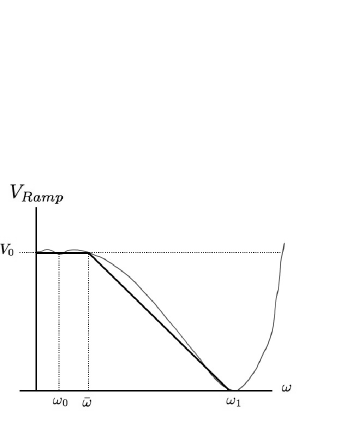
Figure 8: The ramp approximation to the potential of Fig. 7, not to scale. This approximation is a conservative estimate of the true bounce action.

Ref. Lee:1985uv estimated:

$$A \sim \left(\frac{6\,M_{5}^{3}}{k}\right)^{2}\bar{\omega}^{4}$$

$$S_{B} = \frac{32\pi^{2}}{3}\left(\frac{6\,M_{5}^{3}}{k}\right)^{3/2}\frac{\bar{\omega}^{3}}{K},$$ (56)

where $K$ is the ramp slope and the factors of $6M_{5}^{3}/k$ take into account the non-canonical normalization of $\omega$.

The escape point $\bar{\omega}$ is determined within our earlier approximations by cancellation of the third and fourth terms of Eq. (40):

$$\frac{\delta\omega_{0}^{2-\alpha_{2}}}{2+\alpha_{2}}\bar{\omega}^{2+\alpha_{2}}\approx\kappa\frac{\omega_{1}^{\gamma}}{4}\bar{\omega}^{4}\longrightarrow\bar{\omega}\approx\omega_{0}\left(\frac{4\delta}{\kappa(2+\alpha_{2})\omega_{1}^{\gamma}}\right)^{1/(2-\alpha_{2})}.$$ (57)

Given Eq. (47), we see that $\bar{\omega}\gg\omega_{0}$. We will therefore neglect $\omega_{0}$. The ramp slope is therefore given by:

$$K\approx\frac{V_{0}}{\omega_{1}-\bar{\omega}}\sqrt{\frac{k}{6\,M_{5}^{3}}},$$ (58)

where the square root factor again accounts for the non-canonical normalization of $\omega$.

Assembling the pieces of our bound,

$$N_{bubbles}<e^{30}\left(\frac{6\,M_{5}^{3}}{k}\right)^{2}\frac{\bar{\omega}^{4}}{H_{inflation}^{4}}e^{-\frac{32\pi^{2}}{3}\left(\frac{6\,M_{5}^{3}}{k}\right)^{2}\frac{\bar{\omega}^{3}\,(\omega_{1}-\bar{\omega})}{V_{0}}}<1.$$ (59)

VI 4D $\Pi$ Effective Field Theory

VI.1 Integrating Out The Waterfall

During inflation, when $\cos\left(\frac{\Pi}{2f_{\pi}}+\sigma\right)\sim-1$, the physical radion mass-squared at its metastable point $\omega\sim\omega_{0}$ is of order $\delta\omega_{0}^{2}\,k/(12\,M_{5}^{3})$, since we have arranged that the potential in this region is dominated by the second and third terms of Eq. (40). By Eq. (43), it follows that the radion is heavier than $H_{inflation}$. This justifies integrating $\omega$ out during inflation and considering the simple one-field slow-roll potential for $\Pi$ and comparing it with the standard single-field inflation requirements.

The dominant effect of integrating out $\omega$ is classical and involves extremizing $V_{eff}(\Pi,\omega)$ with respect to $\omega$ for constant fixed $\Pi$, and then plugging this $\omega_{infl}(\Pi)$ back into the potential. During inflation the two-field potential is well approximated by:

$$V(\omega,\Pi)\approx-\frac{\delta\omega_{0}^{2-\alpha_{1}}}{2+\alpha_{1}}\omega^{2+\alpha_{1}}-\cos\left(\frac{\Pi}{2f_{\pi}}+\sigma\right)\frac{\delta\omega_{0}^{2-\alpha_{2}}}{2+\alpha_{2}}\omega^{2+\alpha_{2}}-v_{0}\cos\frac{\Pi}{f_{\pi}}+V_{0}.$$ (60)

Extremizing with respect to $\omega$,

$$\partial_{\omega}V\left.\right|_{\omega_{infl}} \approx -\delta\omega_{0}^{2-\alpha_{1}}\omega_{infl}^{1+\alpha_{1}}-\cos\left(\frac{\Pi}{2f_{\pi}}+\sigma\right)\delta\omega_{0}^{2-\alpha_{2}}\omega_{infl}^{1+\alpha_{2}}=0$$

$$\omega_{infl} \approx \omega_{0}\left[-\cos\left(\frac{\Pi}{2f_{\pi}}+\sigma\right)\right]^{1/(\alpha_{1}-\alpha_{2})}.$$ (61)

Plugging $\omega_{infl}$ back into Eq. (60), taking $\sigma\sim\pi/2$ and expanding to ${\cal O}(\Delta\Pi)^{2}$ (where $\Delta\Pi\equiv\pi f_{\pi}-\Pi$) we find the single-field effective potential:

$$V_{eff,infl}\approx V_{0}-\frac{m_{\Pi}^{2}}{2}(\Delta\Pi)^{2},$$ (62)

$$m_{\Pi}^{2}\approx-\left(\frac{v_{0}}{f_{\pi}^{2}}+\frac{\delta\,\omega_{0}^{4}}{4(2+\alpha_{2})\,f_{\pi}^{2}}\right).$$ (63)

As mentioned earlier, we will choose parameters for which the first term in Eq. (63) dominates. Very near the end of inflation, as the inflaton nears the critical point at which the waterfall potential turns over, these approximations break down. Nevertheless, they are very good during the first few e-foldings when the constraints from precision CMB measurements are most important.

VI.2 Constraining The Slow-roll Potential

In order to discuss constraints from precision cosmology, we begin by defining the usual potential slow-roll parameters Baumann:2009ds :

$$\epsilon \equiv \frac{M^{2}_{Pl}}{2}\left(\frac{V^{\prime}}{V}\right)^{2}\ll 1$$

$$\eta \equiv M^{2}_{Pl}\frac{V^{\prime\prime}}{V}\ll 1.$$ (64)

In models described by Eq. (62) these are approximately:

$$\epsilon(\Delta\Pi) \approx \frac{M_{Pl}^{2}}{2}\frac{m_{\pi}^{4}(\Delta\Pi)^{2}}{V_{0}^{2}}$$

$$\eta \approx M_{Pl}^{2}\frac{m^{2}_{\pi}}{V_{0}}\approx-\frac{M_{Pl}^{2}}{V_{0}}\left(\frac{v_{0}}{f_{\pi}^{2}}+\frac{\delta\,\omega_{0}^{4}}{4(2+\alpha_{2})\,f_{\pi}^{2}}\right).$$ (65)

As is typical in hybrid models $\epsilon<\eta^{2}\ll\eta$, so that the 5-year WMAP measurement of the scalar spectral index indicates the following central value for $\eta$ Komatsu:2008hk :

$$\eta=-0.02.$$ (66)

Measurements of the scale of primordial density perturbations imply the following constraint on the potential Komatsu:2008hk :

$$\left.\frac{V}{\epsilon}\right|_{k_{0}}\approx 5.68\times 10^{-7}M^{4}_{Pl},$$ (67)

where the subscript $k_{0}$ indicates that the quantity is to be evaluated when the scale $k_{0}=0.05\,\textrm{Mpc}^{-1}$ left the horizon. Given the above approximations we can find the number of e-foldings before inflation ends as follows:

$$N(\Pi)\approx\int_{\Pi}^{\Pi_{end}}\frac{V(\bar{\Pi})}{V^{\prime}(\bar{\Pi})}d\bar{\Pi}\approx\frac{1}{\eta}\ln\left(\frac{\Delta\Pi_{end}}{\Delta\Pi}\right).$$ (68)

VII Leading Corrections

We have now worked through the desired behavior of our model, arriving at two-field and one-field effective descriptions with the delicate potentials needed for satisfactory inflation. But we must be careful that there are not uncalculated corrections that follow from our 5D action which could destabilize our story. The fact that the waterfall and inflaton fields are realized as moduli that are non-local from the 5D point of view means that they are insensitive to the short-range effects of whatever very massive physics UV completes our 5D effective theory. Instead we must consider finite loop effects.

The $\Pi$ potential is only sensitive to charged particles that traverse the inflaton throat and are sensitive to the associated Wilson loop observable. But such effects are Yukawa suppressed for massive charged particles, by $e^{-\pi Lm_{5}}$. We are assuming that $\Sigma$ is considerably lighter than other charged fields at the cutoff of the effective description. The cross-coupling with $\omega$ already makes use of a one-way virtual traversal of the inflaton throat ending on boundary/brane localized sources. The leading correction that then involves a virtual “round-trip” in the inflaton throat, Yukawa-suppressed by $e^{-2\pi Lm_{\Sigma}}$, is given by the vacuum loop of $\Sigma$ in the $\Pi$ ($A_{5}$) background, since the diagram is unsuppressed by any further small couplings. But we have already estimated this and we will choose parameters so that it dominates the inflaton potential up to a constant during inflation. Higher corrections will be parametrically smaller. Once the vacuum loop satisfies the slow-roll conditions as discussed in the previous section, they will remain satisfied with the higher corrections.

In the waterfall throat, however, we have only worked at classical order thusfar. The leading corrections to the $\omega$ potential will arise from vacuum loops of the bulk fields that involve virtual round-trips and thereby measure the radius of compactification parametrized by $\langle\omega\rangle$. In the AdS/CFT dual language, our bulk scalar fields correspond to single-trace operators of a large-N type conformal field theory, and the UV brane sources linear in these fields correspond to deformations of the underlying CFT by these single-trace operators. But regardless of the quantum numbers of these operators, the double-trace “square” of such operators cannot be forbidden by symmetry (except possibly supersymmetry which we do not consider). The bulk loop corrections in the waterfall throat capture the effects of these double-trace deformations. The most important double-trace operator in the IR is the one with the lowest scaling dimension. In the leading large-N limit this is given by twice the scaling dimension of the associated single-trace operator. The lowest dimension is dual by AdS/CFT to the lowest mass-squared in the warped throat, namely the tachyon $\chi_{1}$. By (scaling) dimensional analysis from the CFT-side we therefore know that $\chi_{1}$ loops will contribute an $\omega$-dependent term to the effective potential $\propto\omega^{2(2+\alpha_{1})}$.

From the AdS side we get more information. Dimensional analysis for the one-loop correction to the 4D potential says that it must be set by $k^{4}$, since $k$ sets the bulk mass-squared of the tachyon field (for order one $\alpha_{1}$), and the only other scale seen by the small quantum fluctuations (about the classical vacuum profile of the tachyon field) are the brane/boundary masses $\mu$, which we have also taken to be order $k$. Finally, there should be a loop factor $\sim 1/(16\pi^{2})$ multiplying the answer. We thereby estimate a correction

$$\Delta_{loop}V_{eff}\sim\frac{k^{4}}{16\pi^{2}}\omega^{2(2+\alpha_{1})}.$$ (69)

This can be compared with the explicit calculations of Ref. Garriga:2002vf for $\alpha_{1}\ll 1$. We would like this correction to be small enough not to upset our earlier analysis of the $\omega$ potential during inflation. This requires that it is small compared to the other potential contributions $\sim\kappa\omega_{1}^{4+\gamma}$ at $\omega\sim\omega_{1}$. That is, we require

$$\frac{k^{4}}{16\pi^{2}}\ll\kappa\omega_{1}^{\gamma-2\alpha_{1}}.$$ (70)

VIII A Sample Set of Parameters

In this section we collect all of the theoretical and observational constraints on our model. We pick a representative, but not fine-tuned, point in parameter space that satisfies all of these constraints and present the corresponding predictions for cosmological observables. The free parameters in the 4D two field potential are: $\delta$, $f_{\pi}$, $\omega_{0}$, $\omega_{1}$, $\alpha_{1}$, $\alpha_{2}$, $\gamma$, $v_{0}$, $\kappa$ and $\sigma$. Table 1 summarizes the nature of the various constraints on this set of parameters, highlights their location in preceding sections and indicates which parameters they constrain. Table 2 contains a sample set of choices for the 4D parameters as well as corresponding choices for 5D parameters. Table 3 lists the predictions for the CMB and gravitational wave spectrum; i.e. predictions for the inflationary energy density $V_{0}$, the Hubble constant during inflation $H$, the scalar spectral index $n_{S}$, the running of the scalar spectral index $\frac{dn_{S}}{d\ln k}$ and the scalar-to-tensor ratio $r$.

Nature of Constraint	Equation Number(s)	$\delta$	$f_{\pi}$	$\omega_{0}$	$\omega_{1}$	$\alpha_{1}$	$\alpha_{2}$	$\gamma$	$\kappa$	$v_{0}$
$V_{0}$ dominates	41				✔			✔	✔
Separated minima	43, 44, 46, 47	✔		✔	✔		✔	✔	✔
No tachyon blow-up	42	✔
Tachyon-Loop Corrections	70				✔	✔		✔	✔
Reheat temperature	51, 52				✔			✔	✔
Slow-roll parameters	VI.2, VI.2	✔	✔	✔	✔		✔	✔	✔	✔
Spectral index normalization	67	✔	✔	✔	✔		✔	✔	✔	✔
Tunneling suppression	59	✔		✔	✔		✔	✔	✔

Table 1: Summary of theoretical and observational constraints on the parameters of this model. A ✔ indicates that a given parameter is constrained by a particular constraint.

4D Parameter	Sample Value	5D Parameter	Sample Value
$\delta$	$1.9\times 10^{-3}$	$k$	$0.1$
$f_{\pi}$	$2.3\times 10^{-2}$	$M_{5}$	$2\,k$
$\omega_{0}$	$5.3\times 10^{-5}$	$\pi\,L$	$100$
$\bar{\omega}$	$2.4\times 10^{-3}$	$J_{1}$	$2\,k^{5/2}$
$\omega_{1}$	$1.5\times 10^{-2}$	$J_{2}$	$(1.3)\,k$
$\alpha_{1}$	$0.5$	$j_{3}$	$(2.9\times 10^{-5})\,k^{5/2}$
$\alpha_{2}$	$0.6$	$J_{4}$	$2\,k^{5/2}$
$\gamma$	$0.2$	$J_{5}$	$(0.1)k^{5/2}$
$v_{0}$	$8.3\times 10^{-20}$	$J_{IR}$	$(0.3)\,k^{5/2}$
$\kappa$	$3.2\times 10^{-5}$	$J_{UV}$	$(0.3)\,k^{5/2}$
$\sigma$	$\sim\pi/2$	$g_{5}$	$1/\sqrt{2\,k}$
$m_{\omega}^{2}$	$1.3\times 10^{-9}$	$m_{\Sigma}$	$(1.3)\,k$
		$\lambda$	$(0.14)\,k^{4}$
		All $\mu$’s	$k$

Table 2: Sample set of 4D and 5D parameters with all quantities are expressed in $M_{Pl}=1$ units.

Observable	Predicted Value
$V_{0}$	$8\times 10^{-15}\,M_{Pl}^{4}$ or $(7.3\times 10^{14}\,\textrm{GeV})^{4}$
$H_{inflation}$	$5.2\times 10^{-8}\,M_{Pl}$ or $1.3\times 10^{11}\,\textrm{GeV}$
$T_{RH}$	$\lesssim 5\times 10^{-6}\,M_{Pl}$ or 1$\times 10^{13}\,\textrm{GeV}$
$n_{S}-1$	$-0.04$
$\frac{dn_{S}}{d\ln k}$	$7.7\times 10^{-4}$
$r$	$1.6\times 10^{-7}$

Table 3: Predictions for cosmological observables from the parameters in Table 2.

IX Discussion

We have realized four-dimensional slow-roll hybrid inflation as the long-wavelength limit of a controlled five-dimensional effective field theory, and presented a viable sample set of parameters. The maximal scale we invoke in our 5D model is the reduced 5D Planck scale, $M_{5}$. With this choice, non-renormalizable 5D quantum gravity amplitudes become strongly coupled at $\sim(16\pi^{2})^{1/3}M_{5}$. Our fundamental 5D parameters with positive mass dimension are chosen to be somewhat smaller than this so that the theory is indeed weakly-coupled. The only other non-renormalizable coupling outside gravity is the 5D gauge coupling $g_{5}$. 5D gauge theory amplitudes become strongly coupled at $\sim 16\pi^{2}/g_{5}^{2}$. Our choice $g_{5}^{2}\sim 1/M_{5}$ means that all our gauge theory calculations are safely below this strong-coupling scale. On the other hand $g_{5}$ is strong enough to satisfy the “gravity as the weakest force” conjecture of Ref. ArkaniHamed:2006dz .

By construction our sample parameter set is not fine-tuned in the usual sense. The related short-distance quantum divergences in standard hybrid inflation, discussed in the introduction, are physically cut off by extra-dimensional separations. Instead viable inflation in our model follows once one is in the right “ballpark” of parameter space. However, given that parameter space is multi-dimensional this in itself constitutes a mild type of tuning. The exception of course is the fine cancellation of the overall 4D cosmological constant, for which our model contains no mechanism.

Three specific mild tunings in our construction are worth noting. One is the fact that the $\alpha_{i}$ are very close, corresponding to a near-degeneracy of the two tachyon fields in the waterfall throat. We have not explained this approximate degeneracy, but it seems clear that it could originate from an approximate symmetry that exchanges the two fields. Such near degeneracy is characteristic of the Goldberger-Wise mechanism in order to avoid having to introduce very small parameters (on the fundamental scale) by hand.

There however remains one parameter which still is notably small, without symmetry protection. While most of the waterfall field terms in our effective potential, Eq. (40), arise from propagation across throats, and are naturally small for small enough sources, the $\omega^{4}$ term is exceptional. As discussed in Section III C it arises purely locally in 5D, from the IR boundary tension being de-tuned from the RS1 value of $24M_{5}^{3}k$. It cannot be too large without making it impossible to satisfy all constraints within effective field theory control. A quick estimate of the technically natural size of this “de-tuning” of the tension is $\geq M_{5}^{4}/(16\pi^{2})$, if one considers loop renormalization of the tension cut off by a mass scale $\sim M_{5}$. Our sample parameter set satisfies this technical naturalness criterion for the $\omega^{4}$ coefficient. But given that $24M_{5}^{3}k\gg M_{5}^{4}/(16\pi^{2})$ we should ask why the IR boundary tension is even close to the RS1 value. Furthermore, while we have realized high-scale inflation by our choice of parameters in this paper, it appears that low-scale inflation requires a much smaller $\omega^{4}$ coefficient, namely an IR boundary tension even closer to its RS1 value. This would violate even technical naturalness. The simplest resolution is to assume that supersymmetry is preserved in the vicinity of the waterfall IR boundary. This in no way commits us to overall supersymmetry, which we know is broken in the inflationary phase. For example supersymmetry breaking may originate on the UV brane without impacting the IR boundary tension. We hope to study a supersymmetric version of our model in future work, with a focus on understanding to what extent low-scale inflation can take place naturally.

We also found that complete suppression of quantum tunneling presented a strong constraint in our search for a viable region of parameter space. This suggests that more typically in our scenario, standard inflation would be accompanied by some regions of space that ended inflation by tunneling during the first few e-foldings. These may lead to significant deviations from scale-invariance in the CMB spectrum on angular scales accessible by future measurements. Again, we hope to return to a fuller treatment of this possibility in future work.

- (1) A. H. Guth, “The Inflationary Universe: A Possible Solution to the Horizon and Flatness Problems,” Phys. Rev. D23, 347 (1981).
- (2) A. D. Linde, “A New Inflationary Universe Scenario: A Possible Solution of the Horizon, Flatness, Homogeneity, Isotropy and Primordial Monopole Problems,” Phys. Lett. B108, 389 (1982).
- (3) D. Baumann, “TASI Lectures on Inflation,” (2009), eprint 0907.5424.
- (4) L. M. Krauss, “New constraints on ”INO” masses from cosmology (I). Supersymmetric ”inos”,” Nuclear Physics B 227, 556 (1983).
- (5) E. J. Copeland, A. R. Liddle, D. H. Lyth, E. D. Stewart, and D. Wands, “False vacuum inflation with Einstein gravity,” Phys. Rev. D49, 6410 (1994), eprint astro-ph/9401011.
- (6) D. H. Lyth and A. Riotto, “Particle physics models of inflation and the cosmological density perturbation,” Phys. Rept. 314, 1 (1999), eprint hep-ph/9807278.
- (7) L. Randall, “Supersymmetry and inflation,” (1997), eprint hep-ph/9711471.
- (8) K. Freese, J. A. Frieman, and A. V. Olinto, “Natural inflation with pseudo - Nambu-Goldstone bosons,” Phys. Rev. Lett. 65, 3233 (1990).
- (9) A. D. Linde, “Hybrid inflation,” Phys. Rev. D49, 748 (1994), eprint astro-ph/9307002.
- (10) N. Arkani-Hamed, H.-C. Cheng, P. Creminelli, and L. Randall, “Pseudonatural inflation,” JCAP 0307, 003 (2003), eprint hep-th/0302034.
- (11) D. E. Kaplan and N. J. Weiner, “Little inflatons and gauge inflation,” JCAP 0402, 005 (2004), eprint hep-ph/0302014.
- (12) J. M. Maldacena, “The large N limit of superconformal field theories and supergravity,” Adv. Theor. Math. Phys. 2, 231 (1998), eprint hep-th/9711200.
- (13) S. S. Gubser, I. R. Klebanov, and A. M. Polyakov, “Gauge theory correlators from non-critical string theory,” Phys. Lett. B428, 105 (1998), eprint hep-th/9802109.
- (14) O. Aharony, S. S. Gubser, J. M. Maldacena, H. Ooguri, and Y. Oz, “Large N field theories, string theory and gravity,” Phys. Rept. 323, 183 (2000), eprint hep-th/9905111.
- (15) E. Witten, “Anti-de Sitter space and holography,” Adv. Theor. Math. Phys. 2, 253 (1998), eprint hep-th/9802150.
- (16) L. Randall and R. Sundrum, “A large mass hierarchy from a small extra dimension,” Phys. Rev. Lett. 83, 3370 (1999), eprint hep-ph/9905221.
- (17) H. L. Verlinde, “Holography and compactification,” Nucl. Phys. B580, 264 (2000), eprint hep-th/9906182.
- (18) J. Maldacena, unpublished remarks.
- (19) E. Witten, Talk given at ITP Santa Barbara conference New Dimensions in Field Theory and String Theory , URL http://www.itp.ucsb.edu/online/susyc99/discussion/.
- (20) E. P. Verlinde and H. L. Verlinde, “RG-flow, gravity and the cosmological constant,” JHEP 05, 034 (2000), eprint hep-th/9912018.
- (21) S. S. Gubser, “AdS/CFT and gravity,” Phys. Rev. D63, 084017 (2001), eprint hep-th/9912001.
- (22) N. Arkani-Hamed, M. Porrati, and L. Randall, “Holography and phenomenology,” JHEP 08, 017 (2001), eprint hep-th/0012148.
- (23) R. Rattazzi and A. Zaffaroni, “Comments on the holographic picture of the Randall-Sundrum model,” JHEP 04, 021 (2001), eprint hep-th/0012248.
- (24) M. Perez-Victoria, “Randall-Sundrum models and the regularized AdS/CFT correspondence,” JHEP 05, 064 (2001), eprint hep-th/0105048.
- (25) R. Contino, Y. Nomura, and A. Pomarol, “Higgs as a holographic pseudo-Goldstone boson,” Nucl. Phys. B671, 148 (2003), eprint hep-ph/0306259.
- (26) G. R. Dvali and S. H. H. Tye, “Brane inflation,” Phys. Lett. B450, 72 (1999), eprint hep-ph/9812483.
- (27) S. Kachru et al., “Towards inflation in string theory,” JCAP 0310, 013 (2003), eprint hep-th/0308055.
- (28) A. R. Liddle and D. Wands, “Microwave background constraints on extended inflation voids,” Mon. Not. Roy. Astron. Soc. 253, 637 (1991).
- (29) L. Susskind, “The anthropic landscape of string theory,” (2003), eprint hep-th/0302219.
- (30) Y. Hosotani, “Dynamical Mass Generation by Compact Extra Dimensions,” Phys. Lett. B126, 309 (1983).
- (31) Y. Hosotani, “Dynamics of Nonintegrable Phases and Gauge Symmetry Breaking,” Ann. Phys. 190, 233 (1989).
- (32) H. Hatanaka, T. Inami, and C. S. Lim, “The gauge hierarchy problem and higher dimensional gauge theories,” Mod. Phys. Lett. A13, 2601 (1998), eprint hep-th/9805067.
- (33) I. Antoniadis, K. Benakli, and M. Quiros, “Finite Higgs mass without supersymmetry,” New J. Phys. 3, 20 (2001), eprint hep-th/0108005.
- (34) H.-C. Cheng, K. T. Matchev, and M. Schmaltz, “Radiative corrections to Kaluza-Klein masses,” Phys. Rev. D66, 036005 (2002), eprint hep-ph/0204342.
- (35) G. von Gersdorff, N. Irges, and M. Quiros, “Bulk and brane radiative effects in gauge theories on orbifolds,” Nucl. Phys. B635, 127 (2002), eprint hep-th/0204223.
- (36) W. D. Goldberger and M. B. Wise, “Modulus stabilization with bulk fields,” Phys. Rev. Lett. 83, 4922 (1999), eprint hep-ph/9907447.
- (37) R. Sundrum, in Physics in D , edited by J. Terning, C. E. M. Wagner, and D. Zeppenfeld (World Scientific, Singapore, 2005), pp. 585 – 630, eprint hep-th/0508134.
- (38) P. Breitenlohner and D. Z. Freedman, “Positive Energy in anti-De Sitter Backgrounds and Gauged Extended Supergravity,” Phys. Lett. B115, 197 (1982).
- (39) H. Davoudiasl, B. Lillie, and T. G. Rizzo, “Off-the-Wall Higgs in the Universal Randall-Sundrum Model,” JHEP 08, 042 (2006), eprint hep-ph/0508279.
- (40) E. W. Kolb and M. S. Turner The Early Universe, (Westview Press, 1994).
- (41) V. Marra, E. W. Kolb, S. Matarrese, and A. Riotto, “On cosmological observables in a swiss-cheese universe,” Phys. Rev. D76, 123004 (2007), eprint 0708.3622.
- (42) G. Lavaux and B. D. Wandelt, “Precision cosmology with voids: definition, methods, dynamics,” (2009), eprint 0906.4101.
- (43) S. K. Blau, E. I. Guendelman, and A. H. Guth, “The Dynamics of False Vacuum Bubbles,” Phys. Rev. D35, 1747 (1987).
- (44) S. R. Coleman, “The Fate of the False Vacuum. 1. Semiclassical Theory,” Phys. Rev. D15, 2929 (1977).
- (45) S. R. Coleman and F. De Luccia, “Gravitational Effects on and of Vacuum Decay,” Phys. Rev. D21, 3305 (1980).
- (46) K.-M. Lee and E. J. Weinberg, “Tunneling Without Barriers,” Nucl. Phys. B267, 181 (1986).
- (47) E. Komatsu et al. (WMAP), “Five-Year Wilkinson Microwave Anisotropy Probe (WMAP) Observations:Cosmological Interpretation,” Astrophys. J. Suppl. 180, 330 (2009), eprint 0803.0547.
- (48) J. Garriga and A. Pomarol, “A stable hierarchy from Casimir forces and the holographic interpretation,” Phys. Lett. B560, 91 (2003), eprint hep-th/0212227.
- (49) N. Arkani-Hamed, L. Motl, A. Nicolis, and C. Vafa, “The string landscape, black holes and gravity as the weakest force,” JHEP 06, 060 (2007), eprint hep-th/0601001.