The ESO/VLT 3rd year Type Ia supernova data set from the Supernova Legacy Survey ^,

Abstract

Aims. We present 139 spectra of 124 Type Ia supernovae (SNe Ia) that were observed at the ESO/VLT during the first three years of the Canada-France-Hawaï Telescope (CFHT) Supernova Legacy Survey (SNLS). This homogeneous data set is used to test for redshift evolution of SN Ia spectra, and will be used in the SNLS 3rd year cosmological analyses.

Methods. Spectra have been reduced and extracted with a dedicated pipeline that uses photometric information from deep CFHT Legacy Survey (CFHT-LS) reference images to trace, at sub-pixel accuracy, the position of the supernova on the spectrogram as a function of wavelength. It also separates the supernova and its host light in $\sim$60% of cases. The identification of the supernova candidates is performed using a spectrophotometric SN Ia model.

Results. A total of 124 SNe Ia, roughly 50% of the overall SNLS spectroscopic sample, have been identified using the ESO/VLT during the first three years of the survey. Their redshifts range from $z=0.149$ to $z=1.031$. The average redshift of the sample is $z=0.63\pm 0.02$. This constitutes the largest SN Ia spectral set to date in this redshift range. The spectra are presented along with their best-fit spectral SN Ia model and a host model where relevant. In the latter case, a host subtracted spectrum is also presented. We produce average spectra for pre-maximum, maximum and post-maximum epochs for both $z<0.5$ and $z\geq 0.5$ SNe Ia. We find that $z<0.5$ spectra have deeper intermediate mass element absorptions than $z\geq 0.5$ spectra. The differences with redshift are consistent with the selection of brighter and bluer supernovae at higher redshift.

1 Introduction

Since the direct detection of the accelerated expansion of the universe 10 years ago (Riess et al., 1998; Perlmutter et al., 1999), constraining the equation of state of the dark energy component responsible for this acceleration has been a major goal of observational cosmology. Type Ia supernovae (SNe Ia hereafter) samples have been gathered at low and high redshift and extensively used for this purpose. When combined with other probes, the picture of a universe dominated by dark energy emerges (Tonry et al., 2003; Astier et al., 2006; Riess et al., 2007; Wood-Vasey et al., 2007; Kowalski et al., 2008).

Over the past five years, the Supernova Legacy Survey (SNLS) has gathered more than 1000 light curves of SN Ia candidates on the Canada-France-Hawaï telescope (CFHT) using megacam (Boulade et al., 2003), thanks to a rolling search technique for discovery and photometric follow up of SNe Ia in four 1 square degree fields (Astier et al., 2006). Spectra of a subset (about half) of these SNe Ia candidates have been observed on various 8 to 10-m class telescopes (VLT, Gemini N and S, Keck I and II). About 50% of spectroscopically observed SN candidates were observed at the VLT.

In this paper, we present the VLT SN Ia spectral set for the first three years of operation of the SNLS. The non SN Ia spectral set, together with a description of the “real-time” operations and procedures will be presented elsewhere (Basa et al., 2009). The spectra shown here were obtained in the period running from June 1st, 2003 up to July 31st, 2006, as part of two large VLT programs . The spectra have been analysed using novel techniques for extraction and identification which have been described in detail elsewhere (Baumont, 2007; Baumont et al., 2008). For each spectrum we provide a redshift estimate. The identification of SNe Ia relies in part on human judgement, using the SALT2 spectral template of Guy et al. (2007) as a guide (see Baumont et al., 2008).

The SN spectra presented here will be used, along with SN Ia spectra obtained at Gemini and Keck telescopes, to build the 3rd year SNLS Hubble diagram. Our primary goal is that the type and redshift of the SNe Ia used for cosmological analysis are secure. In this paper, we consider two classes of events: secure SNe Ia (“SN Ia”) and probable SNe Ia (“SN Ia$\star$”). Studying the statistical properties of these two classes, in order to assess the validity of using SN Ia$\star$ events together with SN Ia events, is therefore a goal of this paper.

SN Ia spectra are a rich source of physical information about their progenitor history and environment. The possibility of evolution among SN Ia populations at low and high redshifts has been the subject of considerable attention in recent years, as more and more SN Ia spectral sets become available (Garavini et al., 2007; Bronder et al., 2008; Foley et al., 2008a; Blondin et al., 2006; Ellis et al., 2008). Recently, evidence has even been found for a demographic evolution among SN Ia populations, resulting in higher stretch, more luminous SNe Ia at higher redshift (Howell et al., 2007; Sullivan et al., 2009). Using SN Ia spectra to compare their physical properties at low- and high-redshift is therefore a useful cross-check when using SN Ia to constrain the expansion history of the universe. In this paper, we take advantage of the large number of high quality spectra obtained at the VLT to build average composite spectra at various phases with respect to maximum light for $z<0.5$ and $z\geq 0.5$. We also compare our average spectra to composite spectra obtained in a similar way with different data sets (Ellis et al., 2008; Foley et al., 2008a) and discuss the significance of the differences found in terms of possible evolution or selection effects.

A plan of the paper follows. In Section 2, we briefly describe the SNLS photometric survey and the VLT spectral observation programs. In Section 3, we summarise the main steps of the data reduction and spectrum extraction. We detail our identification procedure and classification scheme in Section 4. In Section 5, the spectra are individually presented. Composite spectra at $z<0.5$ and $z\geq 0.5$ are built in Section 6. In Section 7, we discuss our sample in the light of other existing SN Ia spectroscopic data. Concluding remarks are made in Section 8.

2 SNLS Observations

2.1 The SNLS imaging survey

The SNLS is composed of an imaging survey devoted to the detection and the photometric follow up of SN candidates, and a spectroscopic survey of a sample of the detected candidates, prioritised for spectroscopy on various telescopes. The imaging survey ran from June 2003, after a period of pre-survey, until June 2008. It was based on the Deep survey of the Canada-France-Hawaii Telescope Legacy Survey (CFHT-LS) (amounting to half of the 474 nights allocated to the CFHT-LS). Full details of the survey can be found elsewhere (Astier et al., 2006). In brief, SNLS observed 4 fields (D1-4) every 3–5 nights during dark/grey time in the $griz$ filters, each field followed for 5-6 lunations per year. Around 1000 well sampled multi-colour light curves of SN Ia candidates have been obtained up to $z\sim 1.1$.

2.2 Spectroscopic follow-up

Spectroscopy of SNLS SN candidates was performed on several 8 to 10-m class telescopes in both hemispheres, namely the VLT, Gemini-N and S, Keck I and II. Almost 50% of SNLS candidates identified as certain or probable SN Ia were spectroscopically observed at the VLT. Howell et al. (2005) and Bronder et al. (2008) describe the SNLS first three years of Gemini spectral data (up to May 2006), while Ellis et al. (2008) present 36 high signal-to-noise ratio (S/N) SN Ia spectra obtained at Keck. In this paper, we focus on spectra taken at the VLT on Cerro Paranal.

Candidate selection for spectroscopic follow-up was based on the multi-band photometry procedure of Sullivan et al. (2006). This selection was performed on the rising part of the light curves, routinely available thanks to the rolling search strategy (see e.g., Perrett et al. 2009). Candidates were generally sent for spectroscopy at, or slightly after, maximum light, which optimised the time budget allocated for spectroscopy. We triggered a target on VLT every three to four days during dark and grey time.

During the first large program (2003-2005), we performed long slit spectroscopy (LSS) of SN candidates on FORS1 for a total of 60 hours of dark/grey time per semester. During the second large program (2005-2007), we observed using both FORS1 and FORS2 with the standard collimator in LSS and multi object spectroscopy (MOS) mode. Most observations were carried out with the 300V grism, along with the GG435 order-sorting filter. Grism 300V was chosen to optimise spectral resolution, spectral coverage and high enough S/N for an unambiguous identification, even for the faintest candidates of our survey ($i^{\prime}_{AB}\sim 24$). Moreover, using the 300V grism for high redshift SNe allows us to study the interesting rest frame UV region of the spectra. The pixel scale is $0.2^{\prime\prime}$ along the spatial axis and 2.65 $\AA$ along the dispersion axis. At 5000 $\AA$, the resolution limit with this setup is $\approx$ 11 $\AA$. The efficiency of the 300V grism peaks around 4700 $\AA$ at a level of $\approx 80\%$. The 300I grism along with the OG590 order-sorting filter was sometimes used for the faintest ($z>0.8$) SNe. Being typically more distant, and due to strong sky emission and fringing beyond 6000 $\AA$, spectra obtained in this way have a much lower S/N than those acquired with the 300V grism.

The slit width was chosen according to the following rule of thumb: “slit width $\approx$ seeing + 0.2^′′”, as a compromise between observing most of the flux from the targeted candidate and limiting the sky background flux. An air mass $\chi<1.6$ was required for each spectroscopic observation. A “blind offset” technique was used to target the candidate, using a bright star located within $<1^{\prime}$ of the target and then offsetting the telescope to position the slit onto the candidate. When possible, the slit position was chosen to observe both the SN and its host. Differential slit losses were corrected by a Longitudinal Atmospheric Dispersion Corrector (LADC). Residual losses are taken into account with the recalibration procedure described in Section 4.2.

All spectra were acquired in Service Observing mode. With a limiting magnitude of $i^{\prime}_{AB}\sim 24$, 3-4 exposures of 750 or 900s were taken for each candidate, with small offsets along the spatial axis ($Y$; the dispersion axis $X$ is horizontal with our setup). Thanks to the regular time sampling of the rolling search, it was possible to acquire most of candidates around or slightly past maximum light.

3 Data processing

Data reduction and spectral extraction were performed in two separate ways. A quick, “real-time” analysis (within a day of acquisition) was used to assess the type and redshift of the candidate (Basa et al., 2009), an essential task for efficiently allocating other candidates to the various telescopes. In parallel, we developed tools “off-line” to cleanly extract the SN from its host. A dedicated pipeline, PHASE (PHotometry Assisted Spectral Extraction), was used for the final reduction and extraction (Baumont, 2007; Baumont et al., 2008). Full details can be found in these papers; we give only a brief description here. All extractions presented in this paper used the PHASE technique.

The PHASE reduction technique improves over the real-time reductions in refinements of the master flat-fields, the dispersion relation, and in the sky estimation. As an example, the 2D dispersion relation is modeled by a fourth order polynomial in $X_{i}$ (and of 2nd order in $Y_{i}$ and $XY_{i}$) to further reduce the residuals. For flux calibration, we build a single average response curve (one for UT1 and one for UT2 as FORS1 moved from UT1 to UT2 in June 2005) from previous individual standard star observations. We prefer using a well controlled average response for the whole set, rather than using a response built from standard star observations of a different night. This is at the expense of absolute flux calibration, as we average out sky transmission variations from night to night, but permits a more robust estimation of the sensitivity function near the blue edge of the order sorting filter.

PHASE extraction uses photometric information on the SN location and host brightness from the deep reference images ($i^{\prime}_{AB}\sim 27-28$) used for building the SN light curves. This allows us to accurately trace the SN position along the dispersion axis on the two-dimensional spectrogram. Moreover, we build a multi-component model of the galaxies present in the slit (including the host, if resolved) by measuring the spatial photometric profiles of these galaxies on the deep stacked reference images projected along the slit direction. We then add a SN component, modeled as a Gaussian of width equal to the seeing of the spectroscopic observation. The location of the SN is accurately known from the light curves. The flux of each component (SN + host and potentially other galaxies in the slit) is a free parameter, the sum of the profile fluxes being normalised to unity. Such a model is built for each column (the dispersion direction is horizontal with our setup) and fluxes assigned to each component in each column $i$ are estimated by a $\chi^{2}$ minimisation where:

$$\chi^{2}=\sum_{j}\Big{(}\frac{F_{i}({\tt Y}_{j})-{\mathcal{M}}_{i}({\tt Y}_{j})}{\sigma_{j}}\Big{)}^{2}.$$ (1)

Here, $\sigma_{j}$ is the error associated with the column pixel data, ${\mathcal{M}}_{i}$ is the multi-component model in column $i$ and $F_{i}({\tt Y}_{j})=F({\tt X}_{i},{\tt Y})$ is the column flux on the 2D spectrogram. We distinguish three types of galaxies:

• PSF: unresolved, point-like galaxies

• EXT: extended, but regularly shaped profiles, e.g. ellipticals

• Mix: extended, but irregularly shaped profiles, e.g. galaxies with spiral arms.

We note that the latter two cases are not an accurate indication of the physical morphology of the host galaxy, but instead just model the spatial profile of the host that enters the slit.

In the first case, the galactic component of the model is a Gaussian of width equal to the seeing of the deep reference observation. The seeing variation with wavelength is estimated from standard star spectra as a power law of index $\sim-0.3$, in good agreement with Blondin et al. (2005) measurements on FORS1 spectra. In the second case, the model is the “bolometric” spatial profile (the sum of the galactic profile in all observed filters) as measured on the megacam combined deep reference images. For the third case, we use a mixture of a Gaussian with width equal to the spectroscopic seeing to model the core and the photometric spatial profile to model the extended arms. From a pure algorithmic point of view, this latter case is equivalent to have two distinct galaxies, a point-like source and an extended one.

Host models used to extract our VLT spectra are about equally divided into EXT and PSF models ($\sim 30$% each), with only a few percent of cases being Mix models. In the remaining $\sim 40\%$ of cases, no separate extraction of the SN and the host was possible.

PHASE uses a set of default parameters to select the correct host model and make the extraction as automatic as possible. These parameters include cuts on flux, galactic compactness, extension minimum level, colour variation between the centre and the extended part of the host (identifying “Mix” host types), and a minimum value of the SN to host centre distance to perform a separate extraction (usually 0.15^′′, a bit less than one pixel). These default parameters allow an automatic extraction of most spectra, though the parameters can be adjusted for specific cases. PHASE performance and limitations have been discussed in Baumont et al. (2008) and we refer the reader to that paper.

The main hypotheses in using PHASE are that 1) the PSF is a Gaussian of width equal to the seeing; 2) the coordinates of the SN are accurate; 3) CFHT-LS reference images and VLT spectrograms have comparable seeings; 4) no flux of the SN is present in the reference image. Any deviation from these assumptions result in weak flux losses, increased noise, and contamination of a SN spectrum by its host. PHASE performs well for most spectra encountered. In particular, it succeeds at recovering the SN from the host, even in the case of a SN located close to the host centre (typically $\stackrel{{\scriptstyle<}}{{{}_{\sim}}}1$ pixel): strong correlations between the host and the SN are often unavoidable in standard extractions. Even for “non favourable” cases, such as sub-pixel SN/host separations, both component spectra are recovered and are essentially non correlated. This is a remarkable feature of our pipeline, as most SN spectral extractions are hampered by host contamination in these cases. Nevertheless, if the SN is too close to the host centre (separation less than one fifth of the seeing), no separate extraction is possible. In that case, a host spectral template is used at the stage of identification to estimate the host contamination (see Section 4.3).

A comparison between PHASE and standard extractions has been done and illustrated on a few examples in Baumont et al. (2008). A major difference is that, in PHASE, we do not re-sample the data until the final step of flux calibration. This avoids introducing correlations across pixels and allows us to trace the statistical noise along the reduction and extraction procedure. For the same reason, we also avoid rebinning the data at a constant wavelength step, as is done in most standard spectroscopic reduction pipelines. As a consequence, the final PHASE calibrated spectrum has unequal steps. We have checked that the statistical noise is properly propagated with PHASE by computing $<S/N>$, the S/N per pixel averaged over the whole spectral range, and $<S/\sigma>$, the signal-to-r.m.s. ratio. Here, $\sigma$ is the standard deviation of a group of measurements around a low-order polynomial fit. We find relatively good agreement between these two quantities for PHASE extracted spectra.

4 Spectral analysis

4.1 Redshift determination

Where possible, a redshift is obtained from the host galaxy spectrum using characteristic emission or absorption lines, yielding a typical uncertainty of 0.001 on the redshift (Baumont et al., 2008). When no lines are detected, the redshift is determined from the fit of a model to the SN spectrum (see Section 4.2). The typical redshift uncertainty is then $\delta z\approx 0.01$, due to the diversity of ejecta velocities among SNe Ia, (e.g. Hachinger et al. 2006). In about 80% of cases, the redshift is obtained from host emission and/or absorption lines. In SNLS we have two independent identification pipelines. The redshifts (as well as identifications, see below) have been carefully cross-checked using the two-dimensional data to match host lines. Checking the corresponding noise map, “bright” spots visible on the 2D frames are easily identified as true emission lines or cosmic/sky subtraction residuals.

4.2 Identifying SNe Ia

To identify SNe Ia, we use a minimisation procedure using the SALT2 spectral template of Guy et al. (2007) with a combined fit of the light curves and the spectrum consistently performed (Baumont et al., 2008). As the training sample of the SALT2 model only contains SN Ia spectra and light-curves, it does not allow a direct identification of non-SN Ia objects. However, the best-fitting parameter values obtained when fitting a non-SN Ia with SALT2 are in themselves an indirect indication of the SN type (see Section 5.4). In addition, a $\chi^{2}$ template-fitting code (Howell et al., 2005) has been used for cross-check. Both techniques use varying levels of human judgement.

The main output parameters of the SALT2 fit are 1) the light curve fit parameters $x_{0}$ (overall normalisation), $x_{1}$ (light curve shape), and colour $c$, and 2) spectroscopic fit parameters: the host fraction $f_{gal}$ in the model when relevant, and recalibration parameters. The latter enter a recalibration function applied to the photometric model in order to fit the spectrum and account for possible errors in flux calibration (Guy et al., 2007). This function is a polynomial of order $n$, with coefficients $\gamma_{n}$ inside an exponential (to ensure positivity). We usually only use two recalibration parameters: an overall normalisation $\gamma_{0}$ and a first order coefficient $\gamma_{1}$ (tilt applied at rest frame 4400 $\AA$), adding higher order corrections for a few objects. The $x_{1}$ parameter is a light curve shape parameter that can be converted into a stretch factor $s$ or $\Delta m_{15}$ parameter of Phillips (1993); see Guy et al. (2007). The colour $c$ parameter is defined as the difference between $(B-V)_{SN}$ and the average $<B-V>$ value at maximum light for the whole training sample of SALT2.

There are some advantages in using SALT2 as a tool for identification. First, the fit of the light curve yields the date of maximum light. The phase $\phi$ of the spectrum (the number of rest frame days between the date of $B$-band maximum and the date of acquisition of the spectrum) is accurately known, usually within a fraction of day. This alleviates possible degeneracies between SN types, such as between pre-maximum Type Ic supernovae (SNe Ic) and post-maximum SNe Ia, whose spectra show similarities. Second, the training set of the SALT2 model is built from a large collection of spectra and light curves from local and distant SNe Ia. These latter include SNLS SNe themselves, added to the training sample once identified. Third, using a model instead of a set of spectrum templates (as is typical of standard identification techniques) alleviates the problems due to unavoidable incompleteness in phase and wavelength coverage of the template libraries: all SNe are treated on an equal footing. Note also that only SNe typed as SN Ia (as opposed to SNIa$\star$) are included in the training set of SALT2. As an erroneous typing of a SN Ic as a SN Ia is very unlikely, this limits the chance of polluting the training sample. Even in such unlikely case, SALT2 being a model, it is robust against the inclusion of a non-SN Ia object.

Once the SALT2 fit is performed, the identification is guided by the best-fitting spectral parameter values. As the phase is fixed by the light curve fit, the spectral fit implicitly uses the photometry. However, we will not classify a SN candidate as a certain SN Ia if we do not get an adequate fit of the spectrum, even if the light curve fit is good. On the contrary, a convincing spectral fit is sufficient for an SN Ia identification, even if the light curve fit is poor. Our goal is to obtain a clean, spectroscopically confirmed, SN Ia sample.

4.3 Host galaxy subtraction

Spectroscopic identification of distant SNe is challenging. One of the key issues discussed in the literature is host contamination. Low S/N spectra are common, either due to high redshift or because sometimes candidates are observed at a late phase (up to a few weeks past maximum) due to telescope scheduling. Several techniques have been developed to improve host–SN separation. Standard techniques involve template $\chi^{2}$ fitting (e.g., Howell et al. 2005; Lidman et al. 2005) once the spectrum has been extracted, and/or cross-correlation methods, such as the SuperNova IDentification (SNID) algorithm (Blondin & Tonry, 2007), used for the first two years of the ESSENCE project (Matheson et al., 2005; Foley et al., 2008b). Blondin et al. (2005) proposed a PSF deconvolution technique that separates the two components, provided that the spatial extension of the Gaussian profile is very different for the SN and for its host. Zheng et al. (2008) use a principal component analysis decomposition, combined with template fitting to assess the level of host contamination.

SNLS has a key advantage in that deep photometric $ugriz$ data are available for the host galaxy that can assist with SN–host separation. Bronder et al. (2008) used deep $i_{M}$-band photometry to estimate host contamination. More recently, Ellis et al. (2008) used the multi-colour SNLS photometry to do a more sophisticated estimate of host contamination in extracting Keck SNe Ia spectra. This approach is very efficient at removing the host contribution. Though a wide range of host templates are used and are colour-matched to the host galaxy photometric data, it nevertheless has the drawback of using synthetic templates. By contrast, PHASE, while relying on photometric priors, does not use fixed host templates (Baumont et al., 2008).

PHASE measures the photometric profile of the host and, once combined with a PSF model for the SN placed at the SN position, estimates the flux of each component in each pixel along the SN trace on the spectrogram using a $\chi^{2}$ minimisation procedure. Inspection of the residual image after extraction shows that this technique is efficient provided the centre of the two components is separated by more than $\sim 0.15^{\prime\prime}$ and the seeings of the reference and spectroscopic images are similar. Baumont et al. (2008) have shown that fitting a SN spectrum extracted separately from its host, with a SN+host SALT2 model, yields a small amount of residual galactic contribution, i.e. less than 10% on average. This is a good hint that our component separation performs well. Note that our technique is designed within the framework of a rolling search (very deep reference images are required) and may not be well suited for other search techniques.

When it is not possible to extract the two components separately, a $\chi^{2}$ fit of the full (SN+host) spectrum using SALT2 is done. SALT2 has been adapted to fit a galaxy template in addition to the SN model whenever a separate extraction of the SN from its host was not possible with PHASE (Baumont et al., 2008). These galaxy templates include Kinney et al. (1996) types, as well as a series of template spectra synthesised using PEGASE2 (Fioc & Rocca-Volmerange, 1997, 1999) ranging from ellipticals to late-type spirals. Templates are ordered in a regular sequence from red to blue spectra and the best-fit model is interpolated between two contiguous templates in the sequence. We do not add emission lines to the PEGASE templates: whenever PEGASE templates are used to model the host contribution, residual emission lines might be found in the host subtracted spectrum. This technique is then essentially comparable to the PCA+$\chi^{2}$ fitting technique used by Zheng et al. (2008) to evaluate the host contamination in the first season of the SDSS-II survey.

At high redshift and/or for SNe close to their host centre, host subtraction remains a difficulty. We find a higher average host fraction for probable SNe Ia (SN Ia$\star$ type) than for certain SNe Ia (SN Ia type) spectra (see Section 5.4), which shows that, as expected, significant host contamination can alter the quality of the identification. A major improvement would be to have a spectrum of the host. We are currently in the process of obtaining “SN free” spectra for those cases in which the subtraction of the host failed. We plan to use those to improve the efficiency of the host subtraction in the final 5-year SNLS sample.

4.4 SN Classification

We classify candidate spectra into six categories adapted from the classification of Lidman et al. (2005). We define SN Ia (certain SNe Ia), SN Ia$\star$ (probable SNe Ia but other types, in particular SNe Ic, can not be excluded given the S/N or the phase of the spectrum), SN Ia_pec (peculiar SNe Ia), SN? (possible SN of unclear type), SN Ib/c and SN II. In this paper, we only present SNe from the first 3 categories:

$\bullet$ A SN Ia classification requires the presence of at least one of the following features: Si ii $\lambda$ 4000 or Si ii $\lambda$ 6150, or the S ii W-shaped feature around 5600 $\AA$. Where these features are not clearly visible, a SN Ia classification is still possible provided that the following criteria are met:

• 1) The overall fit is visually good over the entire spectral range,

• 2) The spectral phase is earlier than about +5 days. At about one week past maximum, it has been noted that SNe Ia and SNe Ic show strong similarities and confusion between types is possible (e.g., Hook et al., 2005; Howell et al., 2005),

• 3) No strong recalibration is necessary to obtain a good fit (typical flux correction less than 20%). A large recalibration usually indicates that the candidate is not a SN Ia, a fact that would also be reflected in unusual photometric parameters (very red or blue colour, i.e. positive or negative $c$ respectively, very high or low $x_{1}$ value).

$\bullet$ Classifying a candidate spectrum as a SN Ia$\star$ implies that no typical SN Ia absorption (Si or S) can be found but that the overall fit is acceptable over a large spectral range and broad features are well reproduced. Spectra of low S/N, or spectra one week (or more) past maximum fall into the SN Ia$\star$ category unless Si ii is clearly seen.

$\bullet$ A spectrum is classified as a SN Ia_pec when spectral features characteristic of under- or over-luminous objects (e.g. Li et al. 2001) are present.

While the SN Ia category represents two thirds of our total sample, the number of SNe identified as “peculiar” is very small, which may reflect selection biases against such events (Bronder et al., 2008). Low-stretch, underluminous SNe Ia are very hard to identify spectroscopically because of their dimness compared to their usually bright host. Moreover, low S/N spectra of peculiar SNe Ia at high redshift may make them harder to identify than their low-redshift counterparts. Finally, our SALT2-based identification is by essence not well suited for handling peculiar SNe Ia (Guy et al., 2007).

As described above, all types presented in this paper have been cross-checked independently using two techniques: PHASE/SALT2, and the code developed by Howell et al. (2005). Difficult spectra were discussed, on a case-by-case basis, until agreement was reached. In case of disagreement, the most conservative typing was chosen. This procedure makes the identification of the SNe Ia presented in this paper homogeneous to the identification of Gemini spectra of Howell et al. (2005) and Bronder et al. (2008). Note however that we do not use here the confidence index (CI) classification of Howell et al. (2005). As a guide, the SNe Ia of the present paper correspond to CI=4 and 5 while our SNe Ia$\star$ correspond to CI=3.

5 Results

5.1 Individual spectra

In this section, we present the spectra of the 124 identified SNe Ia of the SNLS 3rd year VLT spectroscopic survey, along with their identification as SN Ia, SN Ia$\star$ or SN Ia_pec. Only two objects have been identified as SN Ia_pec (SNLS-03D4ag and SNLS-05D1hk). Their properties are described individually in Section 5.3. In the following, we include them into the SN Ia subsample.

Table The ESO/VLT 3rd year Type Ia supernova data set from the Supernova Legacy Survey ^, lists the SN Ia and SN Ia$\star$ spectra and their observing conditions. In some cases, several spectra of the same candidate were taken due to poor conditions at the telescope, or an insufficient S/N for a secure identification. The asterisk in the column $D_{sep}$ denotes cases for which a separate extraction of the SN from the host component was not possible (including, for some candidates, the absence of a detectable host).

Table The ESO/VLT 3rd year Type Ia supernova data set from the Supernova Legacy Survey ^, summarises the results of our identification for each of the 139 spectra corresponding to the whole set of 124 SNe Ia. Name, type, redshift, redshift source, i.e. host (H) or SN (S), phase, host type, fraction of host used in the best-fitting model, and average S/N per 5 $\AA$ bin are given. This latter quantity is computed on the host subtracted spectrum (when relevant) for each SN. PEGASE best-fitting host model is given as a letter for the morphology (E, S0, Sa, Sb, Sc, Sd) followed by a figure between parentheses indicating the age (in Gyrs). When the best-fit is obtained for a Kinney et al. (1996) template, we indicate the two contiguous Hubble types between which the best-fitting galaxy model is interpolated. Note that a host component is always allowed (this includes a null template), even when the SN spectrum has been extracted separately from its host. Where the best-fit is obtained for a model with no host contribution, the label ’NoGalaxy’ is given.

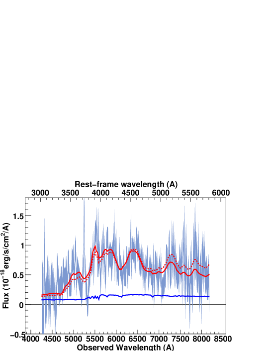
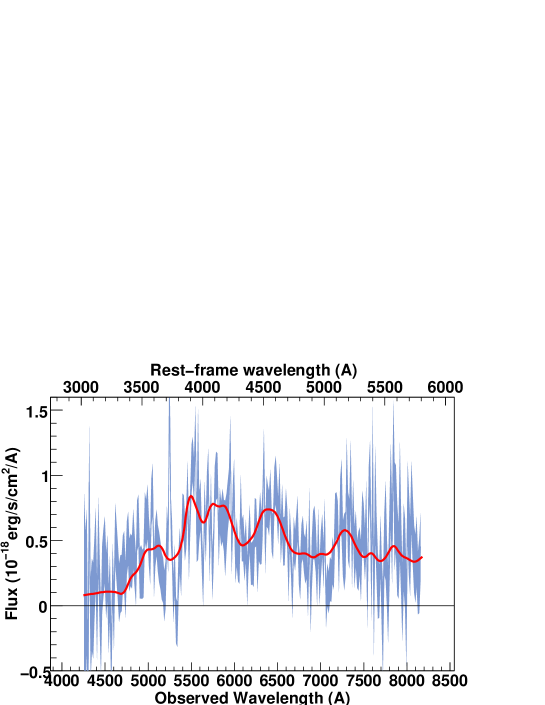
Figure 12: SNLS- 03D1ar270: a SN Ia$\star$ supernova at z=0.408. The spectrum phase is 5.3. A E(7) host model has been subtracted.

Table The ESO/VLT 3rd year Type Ia supernova data set from the Supernova Legacy Survey ^, gives the number of SNe for each class (SN Ia and SN Ia$\star$) per field and in total. Figures 12 to 150 show the full (host+SN) PHASE extracted spectrum (left panel). For each spectrum, the name of the SN is followed by the date of spectroscopy, in terms of the number of days elapsed since January 1st, 2003. The red dashed line is the SALT2 model obtained with no recalibration, the red solid line being the same model after recalibration. Whenever fitting with a host galaxy template is necessary, we show the best-fitting host spectrum model (blue solid line). In these cases, we present in the right panel the host subtracted SN spectrum obtained by subtracting the host model (blue solid line in left panel) from the PHASE extracted spectrum. The best-fit, recalibrated, SN Ia model (solid red line) is overplotted on the host-subtracted SN spectrum.

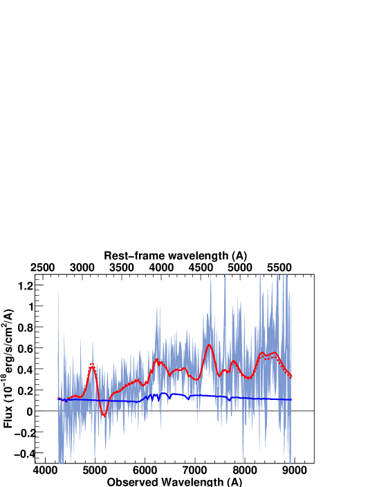
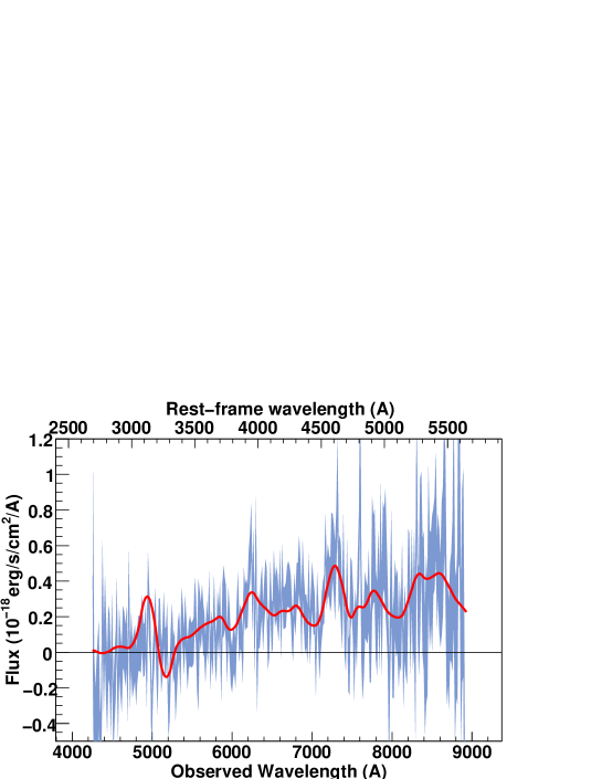
Figure 30: SNLS- 03D4gf329: a SN Ia$\star$ supernova at z=0.580. The spectrum phase is 20.4. A S0(1) host model has been subtracted. The UV part of the model is poorly constrained due to the lack of UV templates at late phases in the version of the SALT2 training set used in this work.

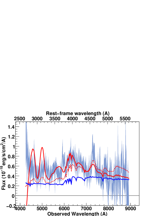
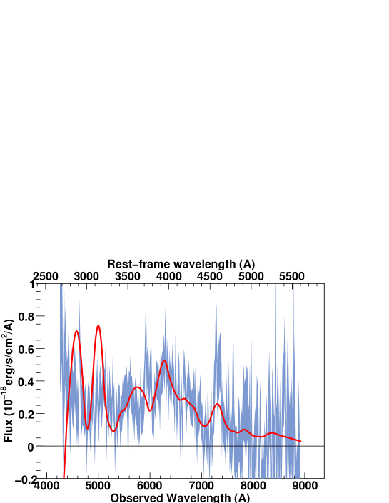
Figure 31: SNLS- 03D4gg330: a SN Ia$\star$ supernova at z=0.592. The spectrum phase is 16.4. A Sc(10) host model has been subtracted. The UV part of the model is poorly constrained due to the lack of UV templates at late phases in the version of the SALT2 training set used in this work.

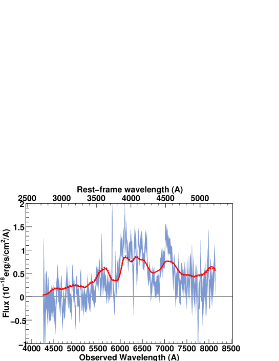
Figure 38: SNLS- 04D1hx628: a SN Ia supernova at z=0.560. The spectrum phase is 5.9. Best-fit obtained for a model with no host galaxy component. Note the model is unable to reproduce the large feature at rest-frame 4500 $\AA$.

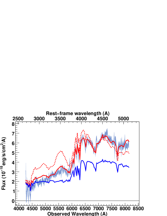
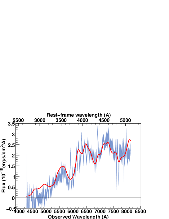
Figure 51: SNLS- 04D1sa716: a SN Ia supernova at z=0.585. The spectrum phase is -2.6. A E(1) host model has been subtracted. Note the bad fit in the UV region due to subtracting too blue a host model.

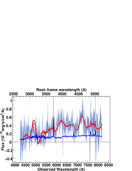
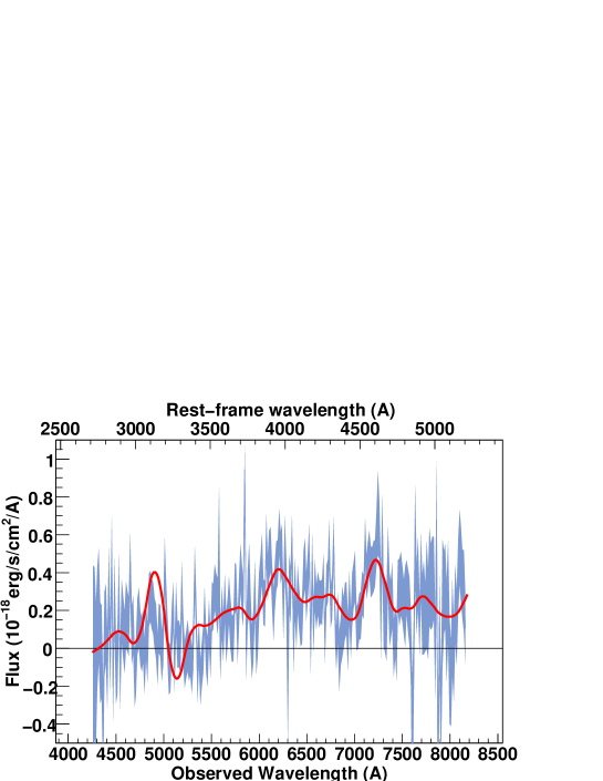
Figure 63: SNLS- 04D2cw445: a SN Ia$\star$ supernova at z=0.568. The spectrum phase is 19.3. A Sb-Sc host model has been subtracted. The UV part of the model is poorly constrained due to the lack of UV templates at late phases in the version of the SALT2 training set used in this work.

As discussed above, host subtraction is a key issue and techniques are not perfect. In particular, the PEGASE templates we use have no emission lines. As a consequence a number of our spectra show residual host lines, e.g., SNLS-04D1sa (Fig. 51) with residual [O ii] emission and Ca ii H&K absorption. In some cases, the fit is poor in some portion of the wavelength range. There can be different explanations for this. In the case of SNLS-04D1hx (Fig. 38), there are two galaxies along the line of sight. The PHASE host model used for the extraction is not accurate, and the extracted spectrum shows strong host residuals. In the case of SNLS-03D4gf, SNLS-03D4gg and SNLS-04D2cw (Figs. 30, 31 and 63), the SALT2 model is unable to reproduce the UV wavelength region due to the lack of UV coverage in the SALT2 training sample used. More specific comments on individual SNe Ia are given in the corresponding caption.

5.2 Average properties of the SN Ia and SN Ia$\star$ samples

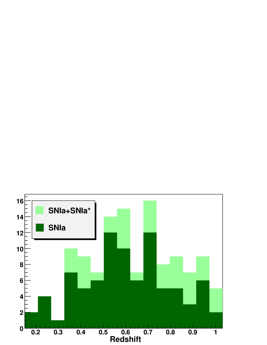
Figure 1: Redshift distribution of SNLS candidates identified as SN Ia or SN Ia$\star$. In light green, the histogram for all SNe Ia (SN Ia+SN Ia$\star$). In dark green, the histogram for SNe Ia alone. The average redshifts for the SNe Ia and SNe Ia$\star$ subsamples are $<z>_{SNIa}=0.60\pm 0.02$ and $<z>_{SNIa\star}=0.70\pm 0.03$ for 86 and 38 SNe, respectively.

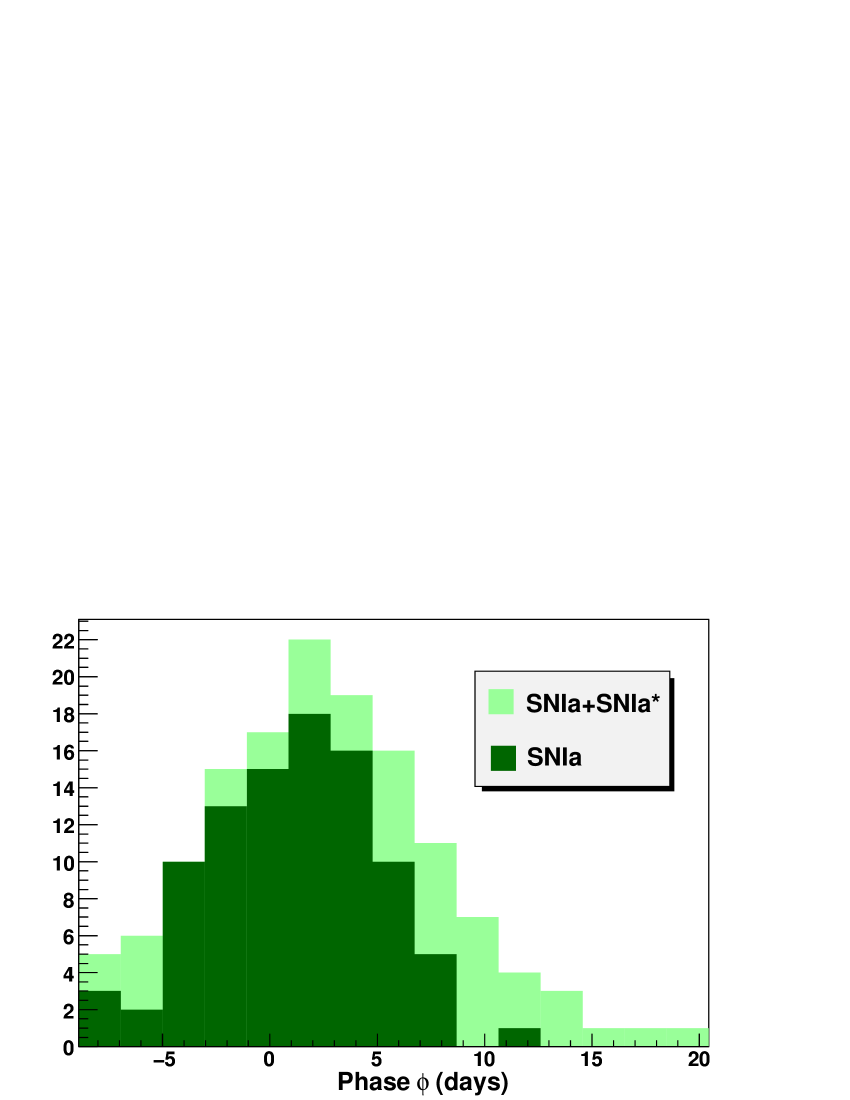
Figure 2: Phase distribution of SNLS candidates identified as SN Ia or SN Ia$\star$. In light green, the histogram for all SNe Ia (SN Ia+SN Ia$\star$). In dark green, the histogram for SNe Ia alone. The average phases for the SNe Ia and SNe Ia$\star$ subsamples are $<\phi>_{SN\leavevmode\nobreak\ Ia}=1.1\pm 0.4$ days and $<\phi>_{SN\leavevmode\nobreak\ Ia\star}=5.8\pm 1.1$ days, respectively.

The main parameters characterizing the SN Ia and SN Ia$\star$ subsamples are given in Table The ESO/VLT 3rd year Type Ia supernova data set from the Supernova Legacy Survey ^, and are discussed below. Figures 1 and 2 show the redshift and phase distributions of both SN Ia and SN Ia$\star$ samples. Redshifts range from $0.149$ to $1.031$. As expected, the SN Ia$\star$ subsample has a higher average redshift ($<z>_{SN\leavevmode\nobreak\ Ia\star}=0.70\pm 0.03$) than the SN Ia subsample ($z_{SN\leavevmode\nobreak\ Ia}=0.60\pm 0.02$). The average redshift of the whole sample is $<z>=0.63$ and the median redshift is 0.62. Below $z\approx 0.3$, all SNe Ia are identified as certain SN Ia.

The average phase of the SN Ia$\star$ subsample is significantly higher ($<\phi>_{SN\leavevmode\nobreak\ Ia\star}=5.8\pm 1.1$ days) than for the SN Ia ($<\phi>_{SN\leavevmode\nobreak\ Ia}=1.1\pm 0.4$ days). This is generally caused by similarities between SN Ia spectra one week past maximum and SN Ic spectra. These cases are labeled SN Ia$\star$ unless Si ii is clearly seen. Fig. 2 shows that most spectra at phases later than 10 days are classified as SN Ia$\star$. This also reflects the lower-S/N in these (fainter) spectra. The average S/N per 5 $\AA$ bin is $\sim 6$ for SN Ia, $\sim 2$ for SN Ia$\star$.

We now compare the rest frame $B$-band magnitudes, at maximum light, for the two samples. For each SN, $m_{B}^{*}$, the apparent rest frame $B$-band magnitude, is determined as part of the light curve fit with SALT2. In order to assess the significance of any discrepancy between the SN Ia and SN Ia$\star$ samples in terms of physical properties of the SNe, we compute, for each SN, the “distance corrected” magnitude $m_{B}^{*c}\equiv m_{B}^{*}-5\log(c^{-1}H_{0}d_{L}(z,\bf\Theta))$, where $d_{L}$ is the luminosity distance, $c$ is here the speed of light and ${\bf\Theta}=\{H_{0},\Omega_{M},\Omega_{\Lambda}\}$ the set of cosmological parameters of the underlying cosmology. Here, we adopt the values ${\bf\Theta}=\{70,0.27,0.73\}$ (Astier et al., 2006). We find $<m_{B}^{*c}>_{SN\leavevmode\nobreak\ Ia}=23.95\pm 0.04$ and $<m_{B}^{*c}>_{SN\leavevmode\nobreak\ Ia\star}=24.12\pm 0.08$. As expected, the SNe we classify as SN Ia$\star$ are fainter, on average, than the ones we classify as SN Ia (by $<\Delta m_{B}^{*c}>=0.17\pm 0.09$ mag). This reflects the fact that low S/N spectra at a given phase fall preferentially into the SN Ia$\star$ category, as they are more difficult to identify.

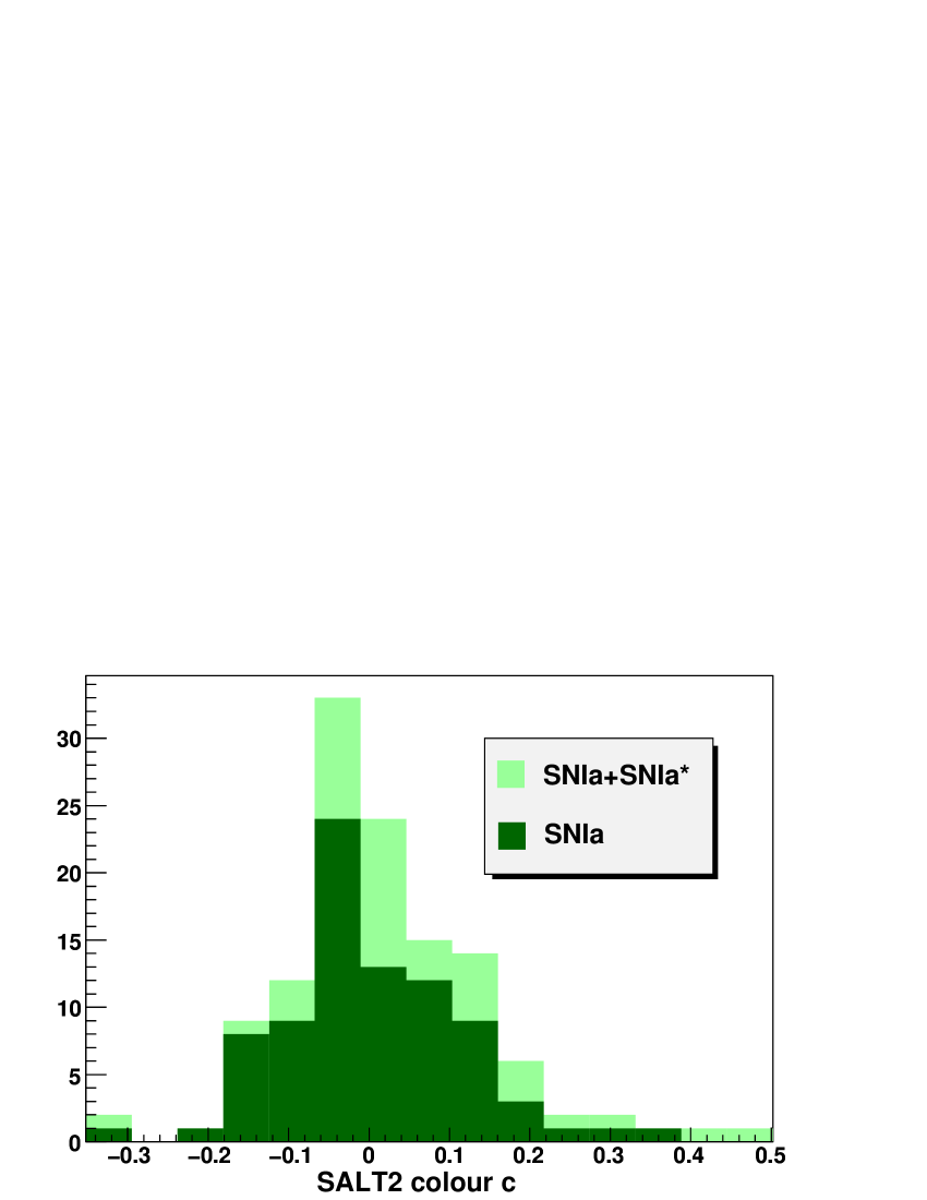
Figure 3: Colour distribution of SNLS candidates identified as SN Ia or SN Ia$\star$. In light green, the histogram for all SNe Ia (SN Ia+SN Ia$\star$). In dark green, the histogram for SNe Ia alone. The average colours for the SNe Ia and SNe Ia$\star$ subsamples are $<c>_{SNIa}=0.009\pm 0.013$ mag and $<c>_{SNIa\star}=0.05\pm 0.03$ mag, respectively.

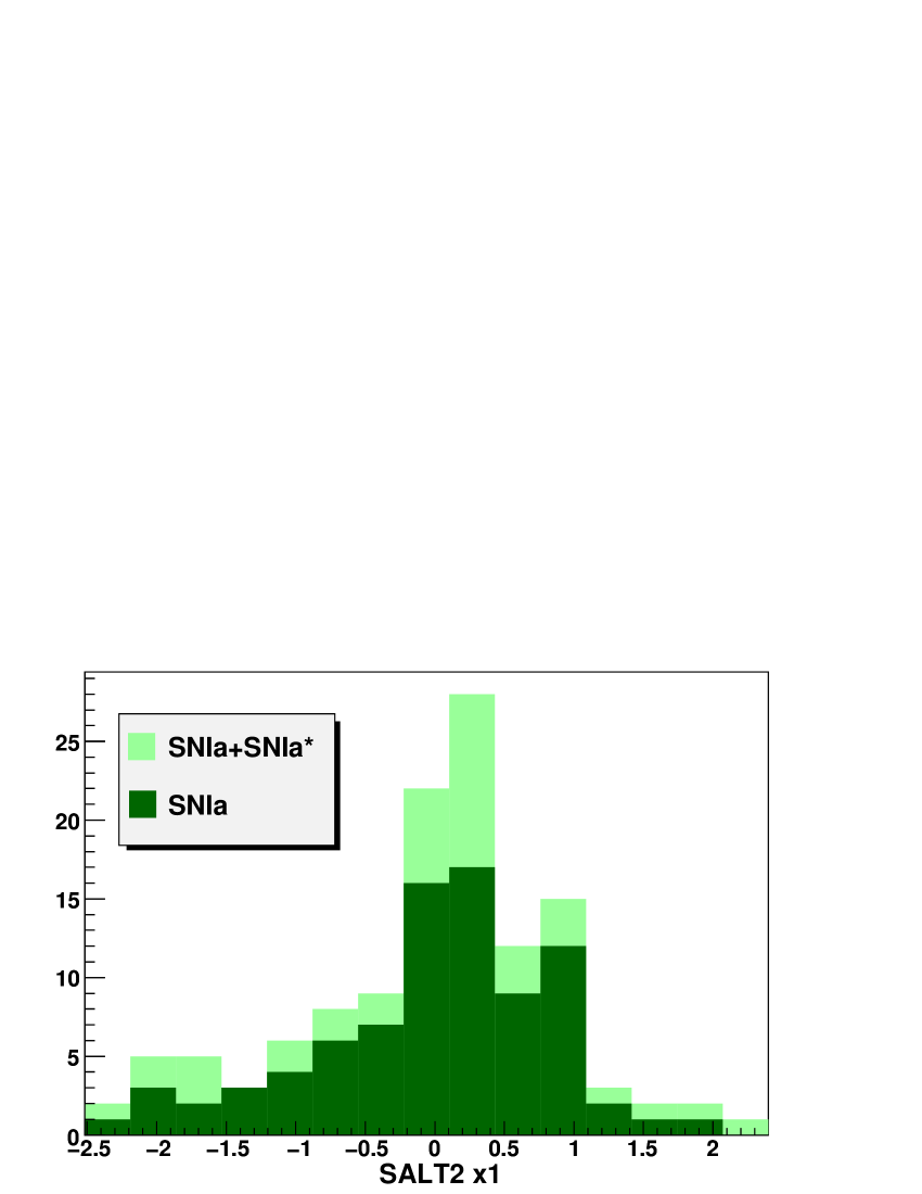
Figure 4: SALT2 $x_{1}$ distribution of SNLS candidates identified as SN Ia or SN Ia$\star$. In light green, the histogram for all SNe Ia (SN Ia+SN Ia$\star$). In dark green, the histogram for SNe Ia alone. The average $x_{1}$ for the SNe Ia and SNe Ia$\star$ subsamples are $<x_{1}>_{SNIa}=-0.02\pm 0.09$ and $<x_{1}>_{SNIa\star}=0.004\pm 0.18$, respectively.

It is of interest to account for the difference found in the $<m_{B}^{*c}>$ values. One obvious explanation is that it is related to the well-known “brighter-slower” (Phillips, 1993) and “brighter-bluer” (Tripp & Branch, 1999) relationships observed in SNe Ia populations. Figures 3 and 4 show the SALT2 colour $c$ and $x_{1}$ parameter distributions for the two subsamples. The SN Ia$\star$ appear to be slightly redder, as their average colour $<c>_{SN\leavevmode\nobreak\ Ia\star}=0.05\pm 0.03$ is higher than for SN Ia: $<c>_{SN\leavevmode\nobreak\ Ia}=0.009\pm 0.013$. Regarding $x_{1}$, we find $<x_{1}>_{SN\leavevmode\nobreak\ Ia}=-0.02\pm 0.09$ and $<x_{1}>_{SN\leavevmode\nobreak\ Ia\star}=0.004\pm 0.18$, which are consistent within $1\sigma$ errors (the SN Ia sample having faster, narrower light curves than the SN Ia$\star$ sample, on average). The “brighter-slower” and “brighter-bluer” relationships translate into a magnitude difference between the two samples of $<\Delta m_{B}^{*c}>=-\alpha_{x}<\Delta x_{1}>+\beta<\Delta c>$. Using $\alpha_{x}=0.13$ and $\beta=1.77$ (Guy et al., 2007), we find $<\Delta m_{B}^{*c}>\approx 0.07\pm 0.06$. The “observed” $<m_{B}^{*c}>$ difference between the two samples is therefore consistent with the “brighter-slower” and “brighter-bluer” relationships. This gives us confidence that our SN Ia$\star$ sample is not significantly polluted by the inclusion of red, non-SN Ia objects, such as SNe Ic. We can estimate the contamination of the SN Ia$\star$ sample by core-collapse SNe by comparing the number of certain SN Ib/c we have typed to the number of certain SNe Ia. In the whole SNLS data, $\sim 3$% of securely identified SNe are of the SN Ib/c type. Applying this ratio to the 38 SN Ia$\star$ of the VLT sample shows that we should expect at most 1 contaminant. Note however that the detection efficiency of the SNLS does not allow us to detect SN Ib/c SNe beyond $z<0.4$ (Bazin et al., 2009). As we only have 3 SN Ia$\star$ with $z<0.4$, this leads to a more realistic estimate of 0.1 SN Ia$\star$ that might be contaminant.

5.3 Peculiar SN Ia

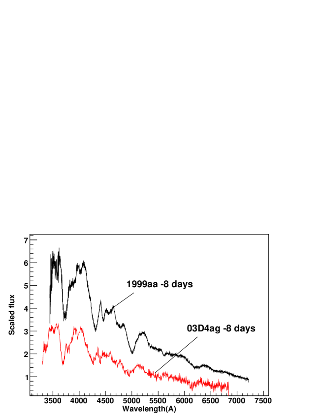
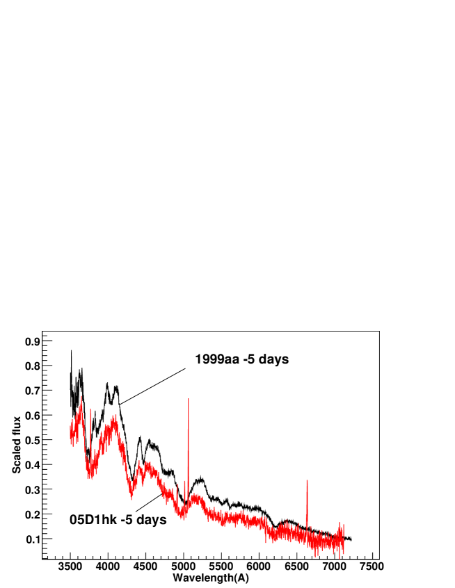
Figure 5: SNLS-03D4ag (top) and SNLS-05D1hk (bottom) rest frame spectra compared to SN 1999aa templates at -8 and -5 days respectively (from Matheson et al. 2008). SN 1999aa spectra are not de-redshifted. None of the spectra are corrected for peculiar velocities, which explains the shifts observed in the positions of absorption features. In both cases, note the very blue spectrum and shallow Si ii $\lambda$ 6150.

We have identified two SN Ia in our sample showing strong similarities with the spectra of SN 1999aa (Garavini et al., 2004) (see Fig. 5). These are 03D4ag and 05D1hk (this latter SN was already noted as a peculiar SN Ia by Ellis et al. 2008). Table The ESO/VLT 3rd year Type Ia supernova data set from the Supernova Legacy Survey ^, summarises the properties of these two SNe as well as the parameters obtained when fitting their spectra with SALT2. Both SNe are at relatively low redshift ($z=0.285$ and 0.263 for 03D4ag and 05D1hk respectively) and at early phase ($\sim-9$ and $\sim-5$ days). 05D1hk has a large $x_{1}$ value, which translates into a $\Delta m_{15}$ parameter (Phillips, 1993) of $0.89$ using the formula given in Guy et al. (2007). By comparison, SN 1999aa has $\Delta m_{15}=0.85$ (Jha et al., 2006). For 03D4ag, we find $\Delta m_{15}=0.97$. Visual inspection of the spectra shows that 03D4ag and 05D1hk have properties typical of high stretch SN Ia: shallow silicon absorption and a blue spectrum, even for the early phases under consideration.

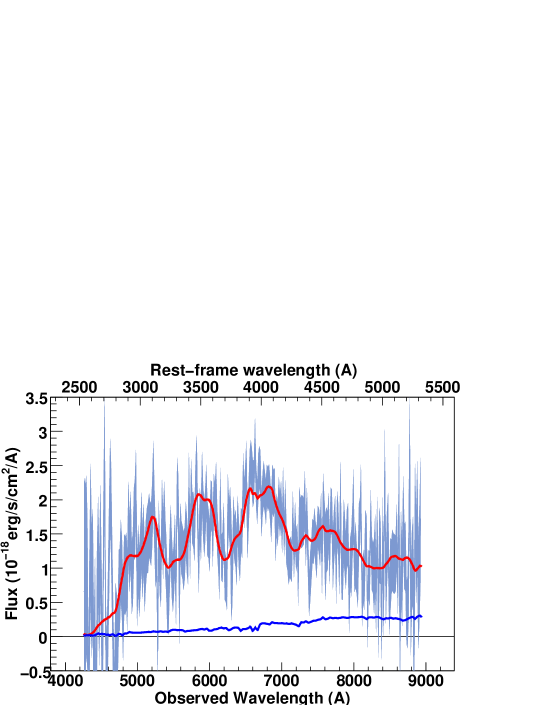
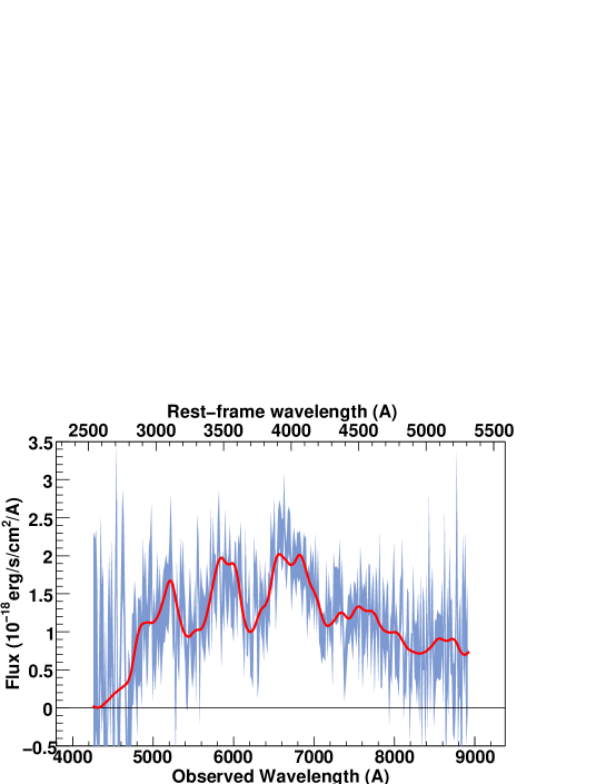
Figure 16: SNLS- 03D1co307: a SN Ia supernova at z=0.679. The spectrum phase is -4.1. A E(8) host model has been subtracted.

The possibility of SNLS-03D1co being a 1991bg-like event has been discussed in Bronder et al. (2008), as there is also a Gemini spectrum of this event. Bronder et al. (2008) found that 03D1co had a large Mg ii $\lambda$ 4300 equivalent width (EW), consistent with the excess absorption measured in under-luminous, low-z SNe spectra. However, the presence of Si ii $\lambda$ 4000 in the Gemini spectrum contradicts this hypothesis, as this feature is not seen in under-luminous SNe because of extra absorption due to Ti ii and Fe ii in the same wavelength range. Based on this observation, Bronder et al. (2008) concluded that 03D1co was likely to be a “normal” SN Ia, in agreement with its normal light curves (Astier et al., 2006). The SALT2 fit of the VLT spectrum of 03D1co confirms this conclusion (see Fig. 16).

5.4 Contamination by non-SN Ia

An obvious challenge in the identification of distant SNe Ia is to avoid confusion with other types, such as SNe Ic, especially one week after maximum light and beyond. Template cross-correlation techniques such as SNID can help (Matheson et al., 2005), but still rely on (unavoidably) incomplete template libraries. Our SALT2 identification procedure provides some additional information on non SN Ia types (or peculiar SNe Ia) through the fitted parameter values, which can differ from those of a typical SN Ia, e.g., an unusually red colour, and/or a high $x_{1}$ parameter, and/or a high recalibration parameter. This is not equivalent to a direct identification of non SN Ia objects, but does allow a mechanism by which peculiar events can be identified. We explore these parameters in this section.

We start with the SALT2 “recalibration parameters” used to adjust the SALT2 photometric model to the observed data. We focus on the first order recalibration parameter $\gamma_{1}$ (Section 4.2). This parameter can be interpreted as the “tilt” required to adjust the observed spectrum to the SALT2 colour model. A large recalibration is a sign that the SALT2 model is not able to properly model the data, as would be the case if we were trying to fit a non-SN Ia spectrum, but could also occur for a SN Ia spectrum whose properties were very different from those of the training sample. Large tilts can also be needed when the host subtraction has failed due to inadequate host modelling or too strong a contamination, although no strong correlation exists between $\gamma_{1}$ and the host fraction.

The average $\gamma_{1}$ value for the SN Ia$\star$ is $<\gamma_{1}>=0.26\pm 0.29$, with $<\gamma_{1}>=0.26\pm 0.11$ for the SN Ia: the required tilts needed to recalibrate the photometric model are only moderate. The dispersions in the $\gamma_{1}$ values are quite large for both samples, with a larger variation for the SN Ia$\star$: $\sigma_{\gamma_{1}}^{SN\leavevmode\nobreak\ Ia}=1.1$ and $\sigma_{\gamma_{1}}^{SN\leavevmode\nobreak\ Ia\star}=1.9$. This can be explained by the inclusion in the SN Ia$\star$ sample of more host-contaminated spectra. If we select only SNe for which a separate extraction from their host was not possible, the mean host fractions $f_{g}$ (i.e. the contribution of the host model to the full spectrum averaged over the whole spectral range) are $<f_{g}>=0.32\pm 0.03$ and $<f_{g}>=0.47\pm 0.05$ for the SN Ia and SN Ia$\star$ subsamples, respectively (see Table The ESO/VLT 3rd year Type Ia supernova data set from the Supernova Legacy Survey ^,). Clearly, spectra identified as SN Ia$\star$ are more host contaminated than SN Ia spectra.

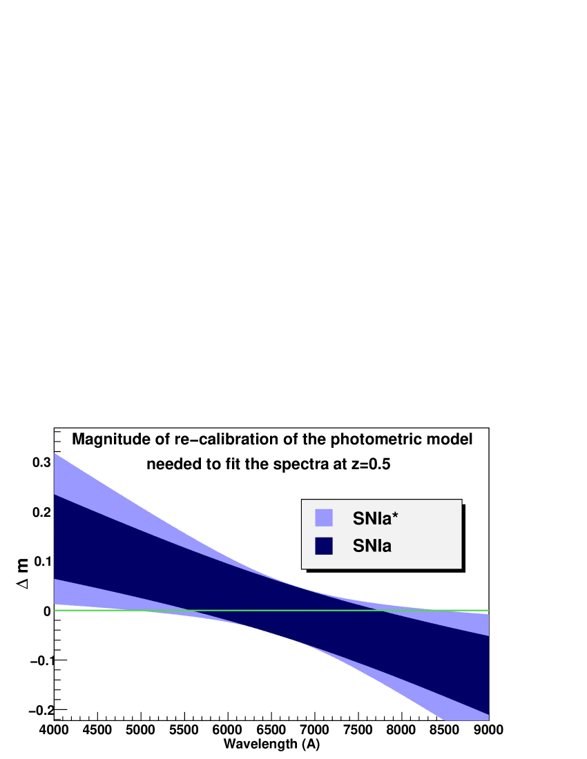
Figure 6: Illustration of the magnitude $\Delta m$ of the average recalibration (“tilt”) needed for the photometric models to fit the spectra, as a function of wavelength. For the purpose of this illustration, we have selected a subset of VLT spectra with redshifts between $z=0.4$ and $z=0.6$. The average redshift is then $<z>=0.512$ for SN Ia and $<z>=0.518$ for SN Ia$\star$. Errors shown in the figure (in light blue for SN Ia$\star$ and in dark blue for SN Ia), are computed from the average value of the recalibration parameter $\gamma_{1}$, estimated from the subset, for both SN Ia and SN Ia$\star$ populations. It appears that, if recalibration is about the same, on average, for SN Ia and SN Ia$\star$ at this redshift, the $\gamma_{1}$ values are more dispersed for the SN Ia$\star$. The global flux correction is mild, $\approx$15% at both ends of the wavelength scale.

We do not find any systematic trend with redshift or phase in the “tilt” values needed to accomodate the SALT2 model with the spectra. In Fig. 6, we show the magnitude $\Delta m$ of the recalibration of the photometric model as a function of wavelength, for a subset of our spectra chosen between $z=0.4$ and $z=0.6$ ($<z>^{SN\leavevmode\nobreak\ Ia}=0.512$ and $<z>^{SN\leavevmode\nobreak\ Ia\star}=0.518$ for this subset). The light blue area is for SNe Ia$\star$, the dark blue one SNe Ia. At this redshift, we find that a $\approx 15$% recalibration is needed at both ends of the effective spectral range, for both the SN Ia and SN Ia$\star$ categories.

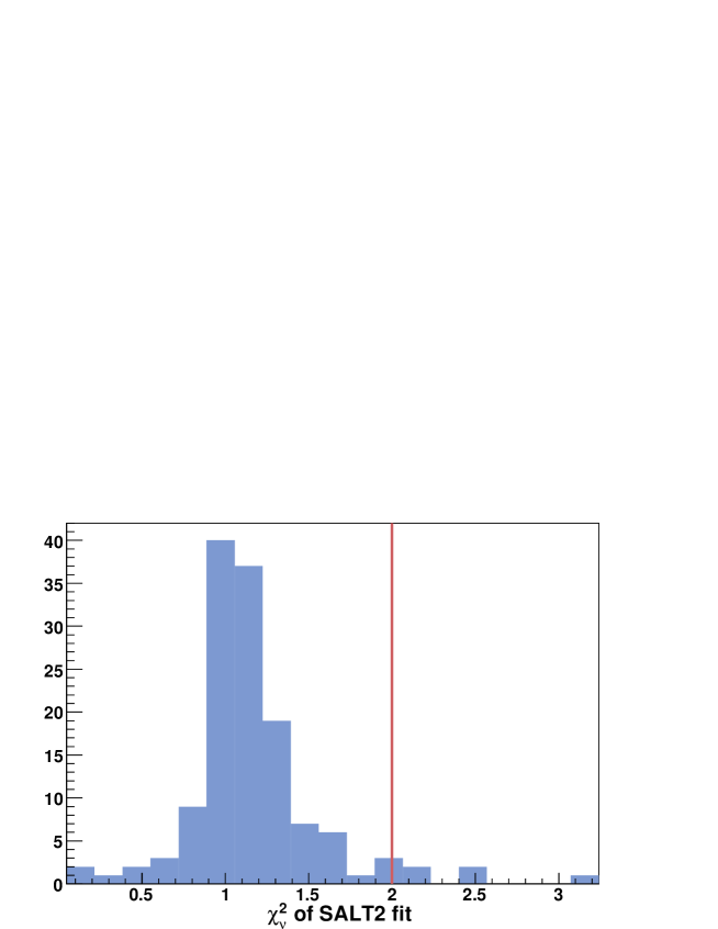
Figure 7: Distribution of SALT2 $\chi^{2}_{\nu}$ values for the whole (SN Ia and SN Ia$\star$) sample. The vertical red/grey solid line indicates the cut at $\chi^{2}_{\nu}=2$ used to identify potential non- or peculiar SN Ia. The two highest $\chi^{2}_{\nu}$ objects are not shown.

A potentially more quantitative criterion is the (reduced) $\chi^{2}_{\nu}$ of the SALT2 spectral fits. We show in Fig. 7 the reduced $\chi^{2}_{\nu}$ histogram of all SALT2 fits (both for the SNe Ia and SNe Ia$\star$ samples). The bulk of the $\chi^{2}_{\nu}$ values are around 1 (or slightly higher), but with a tail of 11 objects with $\chi^{2}_{\nu}>2$ (Fig. 7; the two highest $\chi^{2}_{\nu}$ objects are not shown). With these objects, we find $<\chi^{2}_{\nu}>=1.33$, while excluding them yields $<\chi^{2}_{\nu}>=1.11$. Among the 11 high $\chi^{2}_{\nu}$ objects, one finds 03D4ag and 05D1hk, the over-luminous events identified in Section 5.3. Their best-fit $\chi^{2}_{\nu}$ values are 2.48 and 3.12 respectively. The other objects are (ordered by increasing $\chi^{2}_{\nu}$): SNLS-03D1fc(2.01), SNLS-04D4ht(2.03), SNLS-05D2ct(2.04), SNLS-05D4cw(2.18), SNLS-04D2bt(2.23), SNLS-04D2fs(2.42), SNLS-04D1dc(3.24), SNLS-03D4au(4.63) and SNLS-05D4ff(16.33).

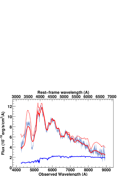
Figure 18: SNLS- 03D1fc358: a SN Ia supernova at z=0.332. The spectrum phase is -4.4. A E(3) host model has been subtracted. Three re-calibration parameters have been used to fit this spectrum.

03D1fc (Fig. 18; SN Ia at $z=0.332$) has a separate extraction from its host. The spectrum has a high S/N and the SALT2 fit parameters are typical of a normal SN Ia. Si ii $\lambda$ 6150 is visible but shallow. The spectrum is not as blue as the one of 05D1hk (which is at about the same phase, i.e. -5 days), but the photometric model requires three recalibration parameters to consistently fit the spectrum. Although the stretch is normal ($s=1.006$), this SN might be slightly peculiar.

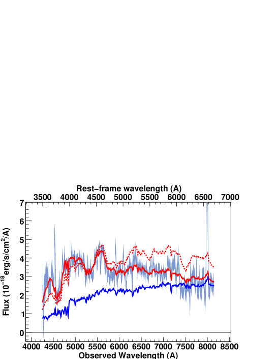
Figure 82: SNLS- 04D4ht628: a SN Ia supernova at z=0.217. The spectrum phase is 6.6. A Sa-Sb host model has been subtracted.

04D4ht (Fig. 82; SN Ia at $z=0.217$) is heavily host contaminated ($>60\%$ of host in the best-fitting model). It has an high colour value ($c=0.5$). 04D4ht is very red but with strong Si ii in its spectrum and is identified as a SN Ia. However, it is located very near the core of its host (a late type spiral) and potentially heavily extinguished.

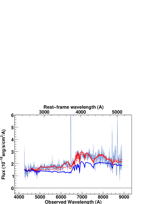
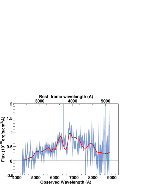
Figure 106: SNLS- 05D2ct799: a SN Ia$\star$ supernova at z=0.734. The spectrum phase is 7.8. A Sd(11) host model has been subtracted.

05D2ct (Fig. 106; SN Ia$\star$ at $z=0.734$) is another example of a SN close to its host centre (more than half of the extracted signal is modeled by a Sd galaxy), slightly red ($c=0.14$) but with a normal stretch ($s=0.994$). It is likely to be extinguished. Due to its fairly high redshift and host contamination, no Si ii is visible either at 6150 or at 4000 $\AA$ and it is identified as a SN Ia$\star$.

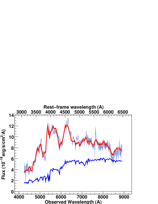
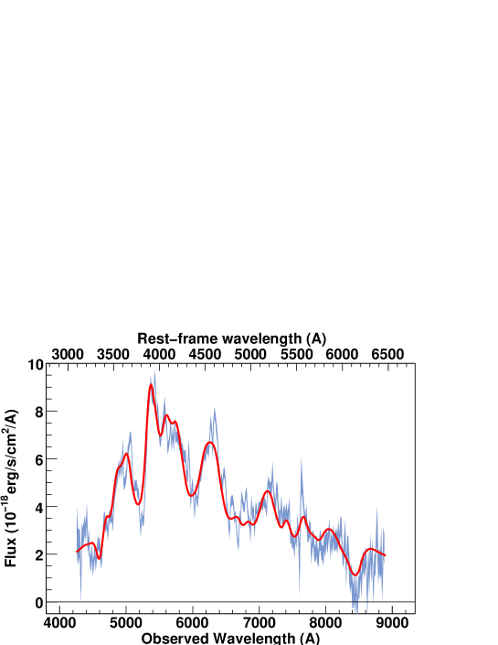
Figure 127: SNLS- 05D4cw950: a SN Ia supernova at z=0.375. The spectrum phase is 7.0. A S0(6) host model has been subtracted.

05D4cw (Fig. 127; SN Ia at $z=0.375$) is a blue ($c=-0.15$) SN. It is heavily host-contaminated, probably an early type galaxy. As it is close to its host centre, a separate extraction was not possible. However, Si ii $\lambda$ 6150 is clearly visible, and it is classified as a SN Ia.

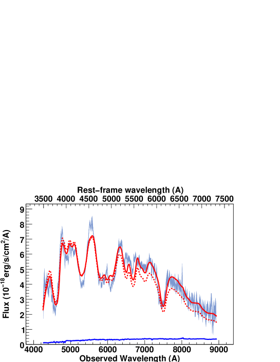
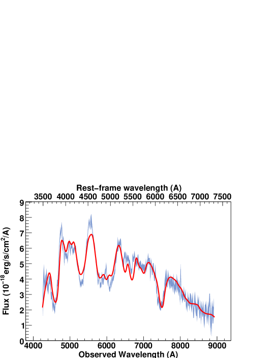
Figure 57: SNLS- 04D2bt444: a SN Ia supernova at z=0.220. The spectrum phase is 6.6. A E(6) host model has been subtracted.

04D2bt (Fig. 57; SN Ia at $z=0.220$) is located in the bulge of its early type host. It is red ($c=0.18$), likely due to host extinction. Si ii and S ii are clearly visible, the classification is SN Ia.

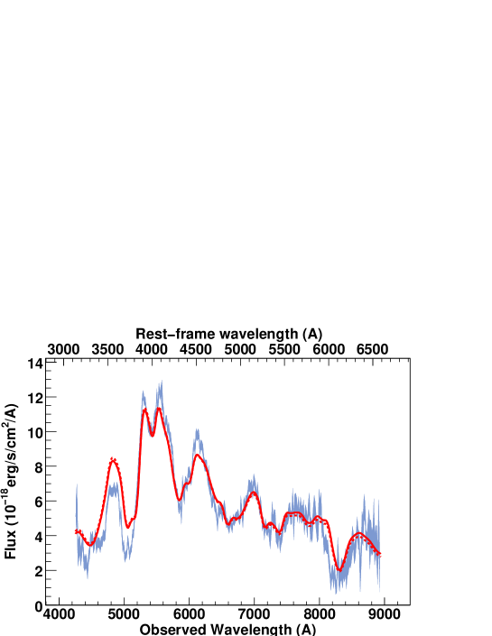
Figure 65: SNLS- 04D2fs470: a SN Ia supernova at z=0.357. The spectrum phase is 1.7. Best-fit obtained for a model with no host galaxy component.

04D2fs (Fig. 65; SN Ia at $z=0.357$) has a large S/N with Si ii and S ii clearly visible. The high $\chi^{2}_{\nu}$ value can be explained by the high S/N (low noise) of the spectrum.

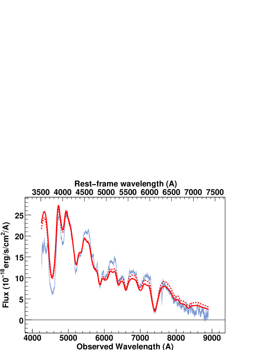
Figure 36: SNLS- 04D1dc589: a SN Ia supernova at z=0.211. The spectrum phase is -0.4. Best-fit obtained for a model with no host galaxy component.

04D1dc (Fig. 36; SN Ia at $z=0.211$) is similar to 04D2fs with a very high S/N. Si ii and S ii are obvious. Again, the high $\chi^{2}_{\nu}$ value reflects the small errors on the spectrum flux.

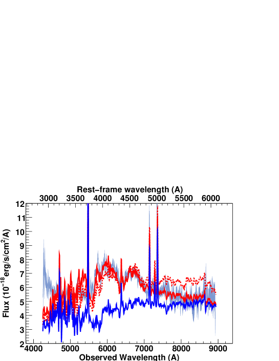
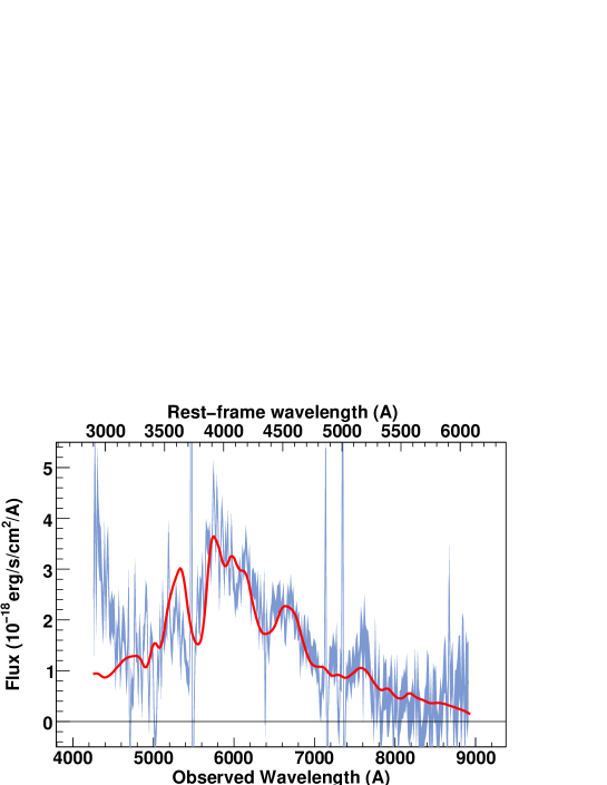
Figure 23: SNLS- 03D4au186: a SN Ia$\star$ supernova at z=0.468. The spectrum phase is 6.5. A Sb-Sc host model has been subtracted. Note the UV flux excess in the spectrum compared to the model. This is due to a host galaxy residual in this region of the spectrum.

03D4au (Fig. 23; SN Ia$\star$ at $z=0.468$) is red ($c=0.18$) and host contaminated, a week past maximum light. It is located right at the centre of its late-type host, probably extinguished, and with strong emission lines that are difficult to subtract, explaining the high $\chi^{2}_{\nu}$ value.

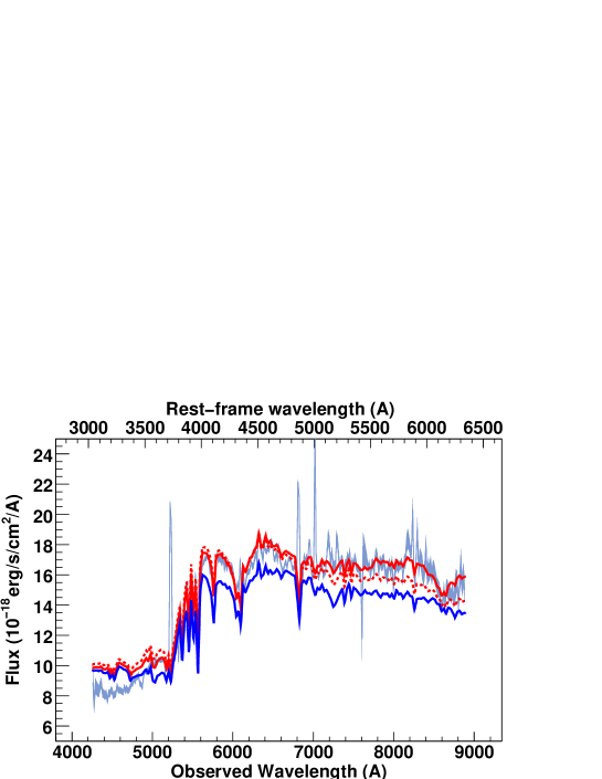
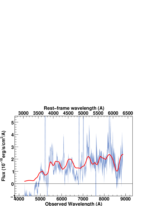
Figure 134: SNLS- 05D4ff1003: a SN Ia$\star$ supernova at z=0.402. The spectrum phase is 5.1. A Sc(6) host model has been subtracted.

05D4ff (Fig. 134; SN Ia$\star$ at $z=0.402$) is heavily buried in its late-type host. The presence of strong [O ii], [O iii] and H$\beta$ emission lines, not present in the host PEGASE template, explains the poor $\chi^{2}_{\nu}$.

In conclusion, a cut in $\chi^{2}_{\nu}$ can help with the identification of peculiar (and possibly non-SN Ia) events, but it is not a straightforward identification. Several effects can conspire to give a high $\chi^{2}_{\nu}$ value, even in the case of obvious SNe Ia. The results of this section suggest that our two subsamples are unlikely to be significantly contaminated by non-SNe Ia.

6 Composite spectra of the SN Ia sample

In this section, we build average VLT spectra in six regions of phase-redshift space to compare the evolution of their properties with redshift.

6.1 Methodology

We select spectra with phase $\phi\leq-4$ days (pre-maximum spectra); $-4<\phi<4$ days (maximum spectra); $\phi\geq 4$ days (post-maximum spectra) for SNe at redshift $z<0.5$ and $z\geq 0.5$, respectively. We only use SN Ia spectra, as the SN Ia$\star$ spectra number in each of the six regions is small and even zero for $z<0.5$ around maximum (since the spectra in this phase-space region are of sufficient S/N and quality to be identified as SN Ia). The number of spectra in each phase bin for both $z<0.5$ and $z\geq 0.5$ is summarised in Table The ESO/VLT 3rd year Type Ia supernova data set from the Supernova Legacy Survey ^,. For the SN Ia spectra, we have 12 pre-maximum spectra (of which 7 are at $z<0.5$), 57 spectra at maximum light (of which 12 are at $z<0.5$) and 24 post-maximum spectra (of which 6 are at $z<0.5$). The average redshift is $<z>=0.36\pm 0.02$ for the $z<0.5$ sample and $<z>=0.70\pm 0.02$ for the $z>0.5$ sample. We have more spectra in the $z\geq 0.5$ bins (68 spectra) than in the $z<0.5$ bins (25), as the median redshift of our sample is 0.62. The spectra of 03D4ag and 05D1hk are excluded from the $z<0.5$ pre-maximum light region, as they have been identified as peculiar SNe Ia (see Section 5.3).

To construct the average spectrum in each region, all individual spectra (shown in the right panels of Fig. 12 to 150 whenever a host model has been subtracted) are brought into the rest frame and rebinned to 5 $\AA$. All spectra are colour-corrected using an up-to-date version of the SALT2 colour law and the colour value $c$ obtained from the SALT2 fit for each SN. Using a Cardelli et al. (1989) extinction law with $R_{V}=3.1$ and $E(B-V)$ values obtained for each SN from their light curve fit, yields very similar results in the wavelength range under consideration. We adopt the SALT2 colour correction in the following. Fluxes are normalised to the same integral in the range 4450-4550 $\AA$. For each wavelength bin, an average weighted flux and its corresponding uncertainty are computed from all spectra included in this bin. Because of the variety of the redshifts involved, the number of spectra entering the average varies from one bin to the other, as does the average phase in a given bin. In practice, the number of spectra in each bin decreases at both ends of the wavelength scale but is approximately constant in the range 4000-7000 $\AA$.

As a consequence of this averaging procedure, the mean phase of the average spectra varies from one wavelength bin to the other. In practice, this variation distorts only very moderately the spectra as the mean phase is roughly the same from one end to the other of the wavelength scale. However, for a given phase range (pre-maximum, maximum or post-maximum), the mean phases of the average spectrum at $z<0.5$ can significantly differ from the corresponding one at $z\geq 0.5$, which should be borne in mind when comparing the average spectrum at $z<0.5$ with that at $z\geq 0.5$. In practice, due to a similar phase sampling of our spectra with redshift, this difference is marginal. We find the following average phases (in days): $\phi^{z<0.5}=-6.1$ and $\phi^{z>0.5}=-5.4$ for pre-maximum spectra, $\phi^{z<0.5}=0.5$ and $\phi^{z>0.5}=0.5$ for spectra at maximum, and $\phi^{z<0.5}=7.7$ and $\phi^{z>0.5}=5.5$ for post-maximum spectra.

6.2 Comparison to Hsiao et al. template spectra

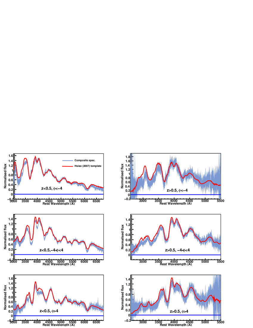
Figure 8: In grey/blue: Average spectrum built from all VLT SN Ia spectra of this study for $z<0.5$ (left column) and $z>0.5$ (right column), and for pre-maximum ($\Phi<-4$ days, top), around maximum ($-4$ days $<\Phi<+4$ days, middle) and past maximum ($\Phi>+4$ days, bottom). To construct the average spectrum in each panel, all individual spectra have been brought into the rest frame and rebinned with 5 $\AA$. Spectra have been colour-corrected using the SALT2 colour law and the colour parameter $c$ for each individual spectrum. Fluxes have then been normalised to the same integral around 4500 $\AA$. For each wavelength bin, an average flux $f_{\lambda}$ and a weighted $1\sigma$ error are computed from all the spectra with measured flux in this bin. The number and average phase thus vary at each wavelength step. In red: an average spectrum built in the same way using this time the Hsiao et al. (2007) template series. For each wavelength bin, the same number of individual templates and same weights as in the average VLT spectrum have been used, with the corresponding phases rounded off to the nearest integer value.

Figure 8 shows the result of averaging the SN Ia spectra (in blue). The left column is for $z<0.5$ spectra, the right for $z\geq 0.5$ spectra. From top to bottom, pre-maximum, maximum and post-maximum spectra are shown. Average spectra built from the Hsiao et al. (2007) template series (red curve) are overlaid on top of the VLT average spectra. Note that about two-thirds of the spectra used in constructing the Hsiao et al. (2007) template are at low redshift ($z<0.1$) and lack UV coverage, so the UV section of the red curves come from the remaining high-redshift spectra used in building the Hsiao et al. (2007) template. In each region of Fig. 8, phases in each wavelength bin are the same for the template and the VLT composite spectrum, weighted in exactly the same way.

The overall agreement between the VLT average spectra and the Hsiao et al. (2007) template is good in all regions. Note that no colour correction has been applied to the Hsiao et al. (2007) templates. As this template is designed for use in light curve fitters that implement “warping” techniques (e.g., SiFTO, Conley et al., 2008), there is no a priori reason that the continuum should agree with our composite spectra. However, we find that the agreement is almost perfect in the optical region of the spectra except around the Ca ii $\lambda$ 3700, Si ii $\lambda$ 4000 and Si ii $\lambda$ 6150 features, for the maximum average spectrum at $z<0.5$. In the UV region, one notices more discrepancies in the fluxes (a low number of spectra are used in this region). Part of this effect might be due to the fact that we normalise the spectra in the optical region. This spectral region is also the most sensitive to differential slit losses. We find a satisfying match of the positions of the UV $\lambda$ 3000 - 3400 features. Note that the peak around 3200 $\AA$ decreases from pre- to post-maximum phases in a proportion that is well reproduced by the Hsiao et al. (2007) model, both at $z<0.5$ and $z\geq 0.5$.

6.3 Comparison of $z<0.5$ and $z\geq 0.5$ spectra

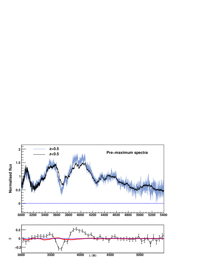
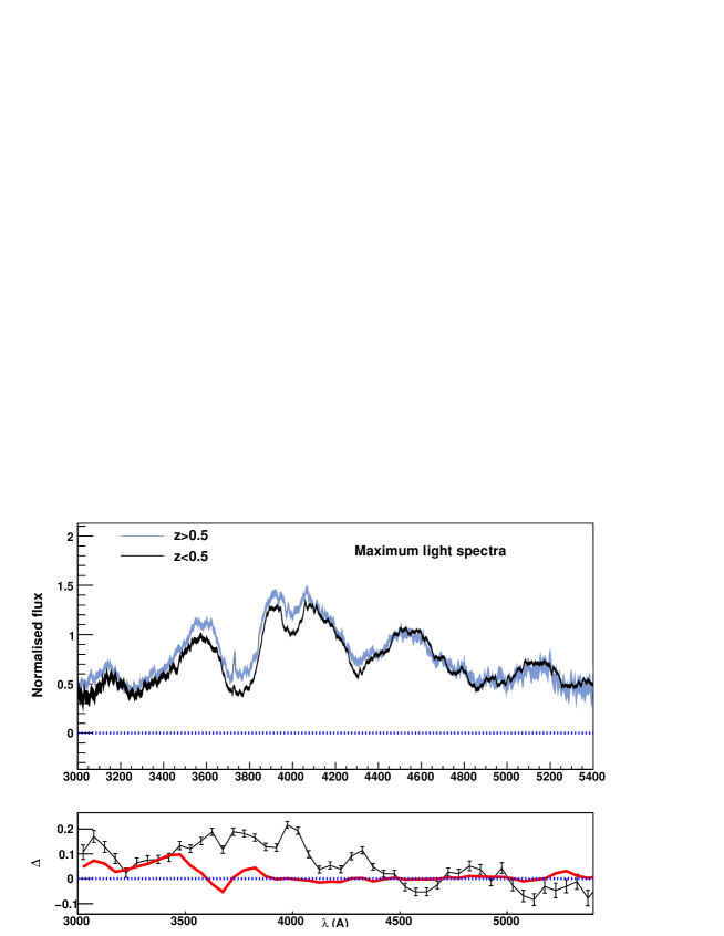
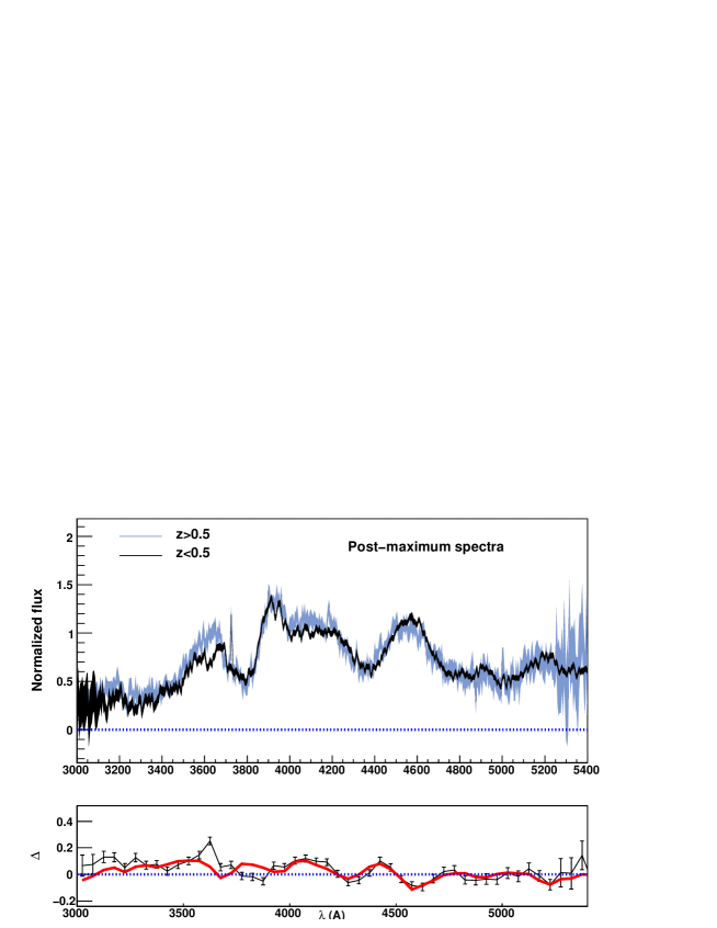
Figure 9: Comparison of $z<0.5$ (in black) and $z\geq 0.5$ (in grey/blue) VLT average spectra for pre-maximum phases (top), around maximum phases (middle), and post-maximum phases (bottom). In each case, the 50 $\AA$ binned residuals $\Delta=f^{z\geq 0.5}(\lambda)-f^{z<0.5}(\lambda)$ are shown for the VLT spectra (in black) and for the Hsiao et al. (2007) templates (in red). For the VLT residual, variances are computed as the quadratic sum of the variances of the two average spectra ($z<0.5$ and $z\geq 0.5$) and $\pm 1\sigma$ errors are shown. Variations in the Hsiao residual (red curves) reflect the different phase mixture of the $z<0.5$ and $z\geq 0.5$ VLT spectra in each wavelength bins. VLT spectra have been individually colour corrected using the SALT2 colour law, recalibrated at the first order using the $\gamma_{1}$ ’tilt’ coefficient and normalised to the same integral in the range 4450-4550Å.

We now compare the average spectra at $z<0.5$ and $z\geq 0.5$ for pre-maximum phases (upper panels of Fig. 9), maximum-light (middle panels) and post-maximum (lower panels). The comparison is done in the region of intersection, from the UV up to the mid-optical wavelengths. For each panel, the blue curve is the $z\geq 0.5$ average spectrum, and the black curve is the corresponding $z<0.5$ spectrum. At the bottom of each panel, we plot the residual $\Delta^{VLT}(\lambda)=f^{z\geq 0.5}(\lambda)-f^{z<0.5}(\lambda)$ (solid black line) with $\pm 1\sigma$ errors.

The mean spectra can be different for two reasons: they might be intrinsically different (i.e. evolution in spectral properties), or the phase distribution of the samples can differ. We therefore compute the residual $\Delta^{Hsiao}(\lambda)$ (solid thick red curve) for the Hsiao et al. (2007) templates shown in Fig. 8. As the underlying assumption in building such spectral templates is that there is no evolution between low and high redshift, $\Delta^{Hsaio}(\lambda)$ should in principle be zero over the whole spectral range. Any deviation from zero, in a given wavelength range, can be attributed to a difference in the average phase of the $z<0.5$ and $z\geq 0.5$ composite spectra in this range. When inspecting differences in the VLT composite spectra at $z<0.5$ and $z\geq 0.5$, it is important to refer to $\Delta^{Hsiao}(\lambda)$: if $\Delta^{VLT}(\lambda)$ follows $\Delta^{Hsiao}(\lambda)$, deviations can be traced back to differing phase distributions of the $z<0.5$ and $z\geq 0.5$ composite spectra. In the opposite case ($\Delta^{VLT}$ is not zero while $\Delta^{Hsiao}(\lambda)$ is zero), any differences should be real.

To quantitatively assess the significance of the differences, we define a reduced $\chi^{2}_{\nu}$ measure of the agreement of the $z\geq 0.5$ VLT composite spectrum and the $z<0.5$ composite spectrum. The variance entering the definition of $\chi^{2}_{\nu}$ is the sum of the variances of the two composite spectra. A value $\chi^{2}_{\nu}\sim 1$ indicates that the two spectra are consistent with one another. We now examine each phase bin in turn.

6.3.1 Pre-maximum spectra

For pre-maximum spectra ($\phi\leq-4$), the composite spectra are typically consistent ($\chi^{2}_{\nu}\approx 1.14$ for 588 degrees of freedom - D.O.F.). The spectra are most discrepant in the UV region (3300 to 4000 $\AA$). A possible explanation is that, as the bands bluer than the rest frame $B$-band are given a lower weight in the SALT2 light curve fit, the colour correction applied to the spectra that uses the colour parameter $c$ derived from the light curve fit, is more efficient in the red than in the blue. Alternatively, this might reflect a greater variability in this spectral region (e.g., Ellis et al., 2008). More variability is expected here due to variations in metallicities of the progenitors, particularly at pre-maximum phases (Hoeflich et al., 1998; Lentz et al., 2000). The residuals in Fig. 9 show the UV region of the pre- and maximum spectra shows more discrepancy than at post-maximum.

6.3.2 Maximum-light spectra

The largest discrepancy between $z<0.5$ and $z\geq 0.5$ is found at maximum light ($-4<\phi<4$). This is the phase where we have the highest number of spectra (12 at $z<0.5$, 45 at $z\geq 0.5$), and the statistical errors are the smallest. We find $\chi^{2}_{\nu}\approx 4.80$ for 601 D.O.F. – the two average spectra are formally not consistent. The largest differences are seen around Ca ii $\lambda$ 3700, Si ii $\lambda$ 4000, Mg ii $\lambda$ 4300 and Fe ii $\lambda$ 4800. Overall, the $z<0.5$ maximum spectrum has deeper absorptions than its $z\geq 0.5$ counterpart.

In the UV up to 3500 $\AA$, the residuals $\Delta^{VLT}(\lambda)$ correlate with the template residuals $\Delta^{Hsiao}(\lambda)$, and the discrepancies between $z<0.5$ and $z\geq 0.5$ may be due to differences in mean phases between $z<0.5$ and $z\geq 0.5$ spectra (recall that due to our averaging procedure, the mean phase varies with $\lambda$ and depends on the phase of the spectra used to build the average spectrum in a given wavelength bin). Around Ca ii $\lambda$ 3700 and beyond, the discrepancies are seen in the spectra, not in the template, and could be real.

Bronder et al. (2008) indicate a possible difference in the EW of Mg ii $\lambda$ 4300 between low and high redshift, but they conclude that it is likely due to differences in the epoch sampling and number of objects at low- and high-redshift. This difference is not found by Foley et al. (2008a) when comparing their composite ESSENCE spectrum with a Lick low-$z$ composite (note that they use a simpler method for host subtraction, which may alter the significance of their comparison). More recently, Sullivan et al. (2009) studied the possible evolution in the EW of intermediate mass elements (IMEs) in the $0<z<1.3$ redshift range. They do not have a Mg ii measurement in their highest-redshift bin, but the predicted variation of Mg ii EW is consistent with zero over their redshift range.

The Si ii-Fe ii-Fe iii $\lambda$ 4800 blend feature is shallower in our $z\geq 0.5$ spectrum than at $z<0.5$, in qualitative agreement with Foley et al. (2008a), who find that this feature is much weaker in their ESSENCE spectrum. They interpret this difference as due to a weaker Fe iii $\lambda$ 5129 line in the high-$z$ spectrum.

The Si ii $\lambda$ 4000 feature is shallower at high redshift, in agreement with the findings of Sullivan et al. (2009). Bronder et al. (2008) do not mention such a difference, but Foley et al. (2008a) find the same kind of trend for Si ii $\lambda$ 6150 (this feature being shallower in their high-redshift ESSENCE spectrum than in the low-redshift Lick spectrum), although they do not mention this for Si ii $\lambda$ 4000. We do not find this difference in our pre-maximum spectra, though it may be present at post-maximum.

6.3.3 Post-maximum spectra

At post-maximum ($\phi\geq 4$), we find a good agreement between the $z\geq 0.5$ average spectrum and its lower $z$ counterpart: $\chi^{2}_{\nu}\approx 1.10$ (547 D.O.F.). Variations in the spectral residuals closely match those in the template residual and reflect mean phase variations between the $z<0.5$ and $z\geq 0.5$ average spectra. Once again, the level of discrepancy, though small, is highest in the UV and in the Si ii $\lambda$ 4000 region. It is interesting to note that, as for the maximum light spectra, the flux at the position of this line (which has almost disappeared a week past maximum) is shallower for $z\geq 0.5$ than for the $z<0.5$ spectrum. For Mg ii $\lambda$ 4300 and Fe ii $\lambda$ 4800, no difference is found with redshift.

Inspection of the spectra shows the presence of a residual [O ii] host line in the $z\geq 0.5$ spectrum, for which a separate extraction of the SN and the host is often difficult. Moreover, our PEGASE host templates do not have emission lines. Other residual absorption (e.g. Ca ii H and K and Balmer lines) is also found in individual spectra.

Our main conclusion of this redshift comparison is that despite the overall agreement between low ($z<0.5$) and high ($z\geq 0.5$) spectral data, some discrepancies are found in characteristic absorption features. This may indicate evolution with redshift, or a signature of some selection effect. We discuss this in the next section.

7 Discussion

In recent years, various large-scale SN programs have published sets of SN Ia spectra at intermediate (Balland et al., 2006, 2007; Zheng et al., 2008; Foley et al., 2008b) and distant (Howell et al., 2005; Lidman et al., 2005; Matheson et al., 2008; Bronder et al., 2008; Ellis et al., 2008; Foley et al., 2008a) redshifts. The SNLS VLT SN Ia spectral data set presented in this paper supplements these existing sets with 124 new SNe Ia, or probable SNe Ia. This constitutes the largest high-redshift SNe Ia spectroscopic sample published so far.

Comparing our data to this literature, we have the highest SN Ia$\star$/SN Ia ratio. Howell et al. (2005) publish the 1st year of SNLS spectroscopy at Gemini. The redshift range targeted is $0.155<z<1.01$, the median redshift being 0.81, higher than our median redshift 0.62. Attributing an index of spectral quality to the Gemini spectra, they identify 34 SN Ia and 7 SN Ia$\star$ among 64 SN candidates (recall that Howell et al. (2005) index CI=4 and 5 to SN Ia and index CI=3 to SN Ia$\star$). Lidman et al. (2005) find 15 SN Ia and 5 SN Ia$\star$ in the range $0.212<z<1.181$ ($<z>\approx 0.5$). In both cases, SN Ia$\star$ amount to $\sim$20% of their total SN Ia sample. We find 86 SN Ia (of which two are SN Ia_pec) and 38 SN Ia$\star$ in our VLT sample, that is $\sim 30$% of SN Ia$\star$. Other surveys such as SDSS-II (Zheng et al., 2008) and ESSENCE (Matheson et al., 2005) both find about 10% of probable SN Ia (equivalent to our SN Ia$\star$). The SDSS-II survey targets low to intermediate redshifts ($0.05<z<0.4$, $<z>\approx 0.22$), which probably makes identification easier. The average redshift of the ESSENCE SNe Ia is $<z>\approx 0.4$ (Foley et al., 2008b), significantly lower than ours.

We identify fewer SN Ia$\star$ towards the end of the SNLS 3rd year period. The average spectroscopic MJD of SN Ia classified spectra is 53393 whereas it is 53272 for SN Ia$\star$ spectra. As all spectra are treated on an equal footing from the point of view of extraction and identification, this can not be due to improvement in data processing or refinements in classification, but more likely indicates an improved target selection efficiency and optimisation of spectroscopic time during the course of the survey.

A key result of this work is the construction of average spectra for various phases and redshift bins from the homogeneous sample of VLT SNe Ia. We have used these high quality average spectra to compare spectral properties at $z<0.5$ and $z\geq 0.5$. We find differences in the depth of some optical absorption features (Si ii and Ca ii) around maximum light. We find that the absorptions due to these elements in the $z<0.5$ spectrum have weakened in the corresponding $z\geq 0.5$ spectrum. Recently, Sullivan et al. (2009) have shown evidence for a similar weakening of singly ionized IME EWs at higher redshift. Using data from various searches, Howell et al. (2007) find an $\sim$8% increase in average light curve width for non-subluminous SNe Ia in the $0.03<z<1.12$ redshift range and interpret it as a demographic evolution. High-$z$ SNe Ia have an average stretch higher than at low redshift, thus are more luminous and hotter, and should ionize more IMEs, depleting singly ionized absorptions in high redshift spectra (e.g., Ellis et al., 2008).

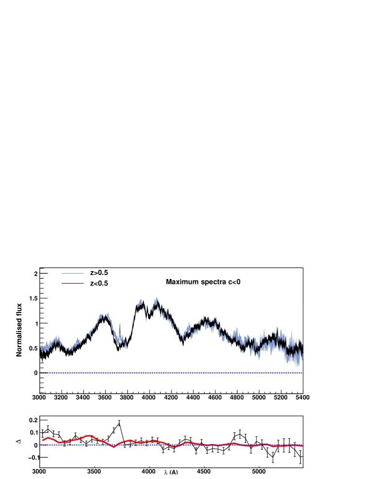
Figure 10: Comparison of $z<0.5$ (in black) and $z\geq 0.5$ (in grey/blue) VLT average spectra around maximum light for bluer than average ($c<0$) subsets (top panel). The 50 $\AA$ binned residuals $\Delta=f^{z\geq 0.5}(\lambda)-f^{z<0.5}(\lambda)$ are shown in the bottom panel for the VLT spectra (in black) and for the Hsiao et al. (2007) templates (in red). For the VLT residual, variances computed as the quadratic sum of the variances of the two average spectra ($z<0.5$ and $z\geq 0.5$) and $\pm 1\sigma$ errors are shown. Compared to the middle panel of Fig. 9, the differences from 3500 to 4500 $\AA$ between $z<0.5$ and $z\geq 0.5$ have been drastically reduced. VLT spectra have been individually colour corrected using the SALT2 colour law, recalibrated and normalised to the same integral in the range 4450-4550Å.

The average stretches of our two redshift subsamples are $<s>^{z<0.5}=0.975\pm 0.017$ and $<s>^{z\geq 0.5}=0.983\pm 0.009$ respectively. These two values are similar given the uncertainties. This is not inconsistent with the results of Howell et al. (2005); Sullivan et al. (2009), as the predicted change in the spectra over our redshift range due to a demographic shift is likely to be very small. The average colours are $<c>^{z<0.5}=0.06\pm 0.03$ and $<c>^{z\geq 0.5}=-0.01\pm 0.01$. The average rest frame distance corrected magnitudes (using ${\bf\Theta}=\{H_{0},\Omega_{M},\Omega_{\Lambda}\}=\{70,0.27,0.73\}$ Astier et al. 2006) are $<m_{B}^{*c}>_{z<0.5}=24.10\pm 0.10$ ($\sigma=0.52$) and $<m_{B}^{*c}>_{z\geq 0.5}=23.88\pm 0.03$ ($\sigma=0.26$), the $z\geq 0.5$ subsample having brighter supernovae, on average, in qualitative agreement with what is expected from Malmquist bias, as brighter supernovae, preferentially selected at higher redshift, tend to be bluer. In order to assess the significance of the apparent spectral differences in our maximum light spectra, we have built two new subsamples (one for each redshift bin) by selecting spectra with phase in the range $-4d<\phi<4d$ and bluer than average (i.e. spectra of SN Ia with colour $c<0$). Using these cuts, we end up with only 6 spectra for the $z<0.5$ bin, and 26 spectra for the $z\geq 0.5$ bin. As we expect to observe bluer objects at higher redshift due to Malquist bias and to the ’brighter-bluer’ correlation, this should select two subsamples with roughly comparable photometric properties. The average distance corrected magnitudes and dispersions of these new subsamples are $<m_{B}^{*c}>_{z<0.5}=23.77\pm 0.04$ ($\sigma=0.11$) and $<m_{B}^{*c}>_{z\geq 0.5}=23.75\pm 0.03$ ($\sigma=0.17$). The two first moments of the $m_{B}^{*c}$ distributions are thus similar. We build new average spectra at maximum light in the same way as in Section 6. The results are shown in Fig. 10 and must be compared to the middle panel of Fig. 9. Most of the differences have diseappeared, except around 3700 $\AA$ and 3900 $\AA$. We find $\chi^{2}_{\nu}=0.97$ (544 D.O.F.). The difference at 3700 $\AA$ is due to a residual [O ii] line in the $z\geq 0.5$. If the differences seen in Fig. 9 were due to imperfect calibration, slit losses or imperfect host subtraction, we would expect to see comparable differences when selecting the two ’blue’ populations shown in Fig. 10. The fact that the composite spectra nicely overlap for these two populations is in itself an indication that the differences with redshift in our maximum light spectra are real. We have checked that the differences remain when selecting a subset of spectra with a host galaxy fraction below 20%. They also remain when we select a subset of spectra with little recalibration ($|\gamma_{1}|<$0.5). Thus it is unlikely that the differences are due to slit losses or a poorer host subtraction at higher redshift. These differences more likely result from the selection of brighter and bluer supernovae at higher redshift.

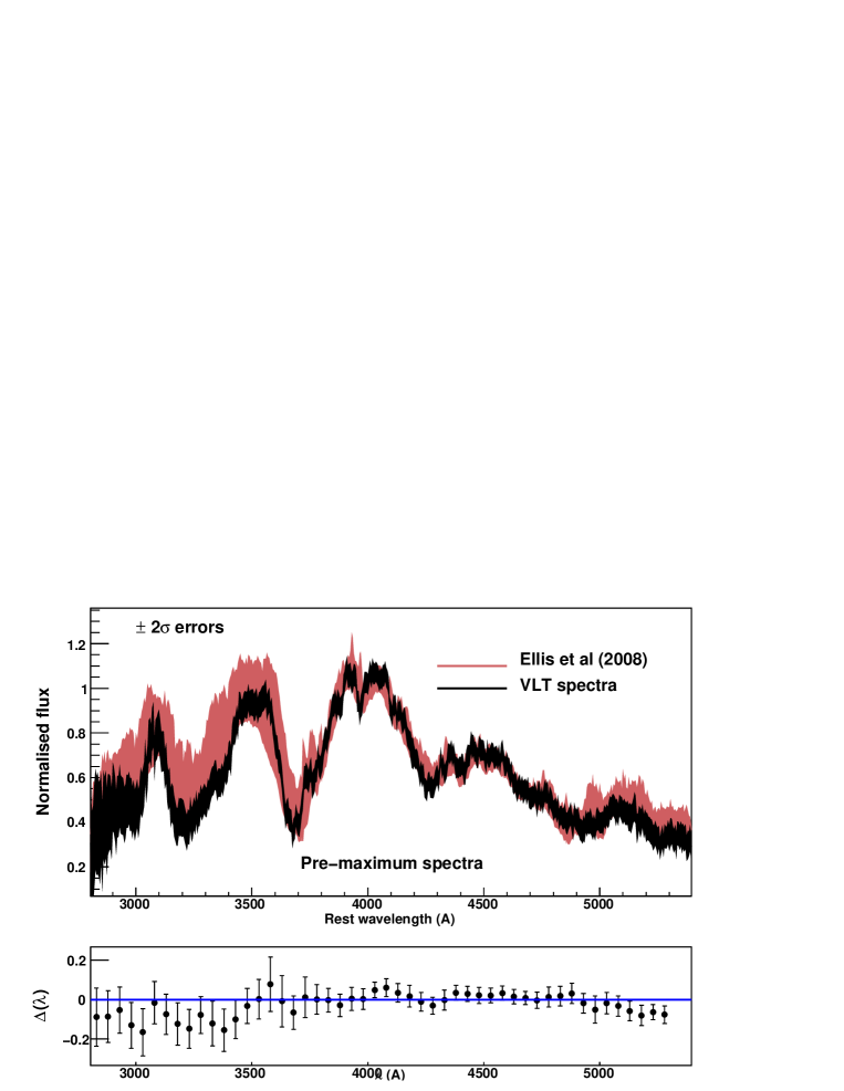
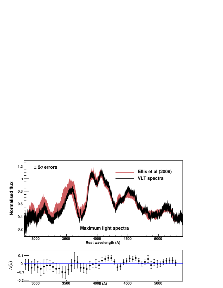
Figure 11: Comparison of the VLT average spectra obtained from a subset of 51 spectra in the range $z=0.35-0.7$ (black), with the Keck average spectra from Ellis et al. (2008) (in grey/red), for pre-maximum phases (top), and at maximum phases (bottom). VLT spectra have been individually colour corrected using the SALT2 colour law and recalibrated at the first order using the $\gamma_{1}$ ’tilt’ coefficient. All spectra have been normalised to unity at 3900 $\AA$. For each phase range, the residuals $\Delta(\lambda)=\Delta^{VLT}(\lambda)-\Delta^{Keck}(\lambda)$ are shown. Variances are computed as the quadratic sum of the variances of the two average spectra (VLT and Keck). Errors are $\pm 2\sigma$.

We now compare our average spectra to the ones of Ellis et al. (2008). These were built from spectra obtained at Keck as part of detailed studies programs using SNLS SNe. Some SNe Ia are common to both samples. We find a qualitative agreement with Ellis et al. (2008) regarding variations in the UV part of the spectra. Figure 11 shows the comparison between a subset of 51 VLT average spectra between $z=0.35$ and $z=0.7$ (with $<z>\sim 0.5$ for this subset), for pre- and maximum phases (in black) with the average spectra obtained from 23 high S/N Keck spectra, with $<z>\sim 0.5$ (in red, from Tables 3 and 4 of their paper). Both VLT and Keck average spectra are shown with lower and upper 2$\sigma$ errors and have been normalised to unity in the same wavelength region (at 3900 $\AA$). VLT spectra have been recalibrated using the SALT2 recalibration function at first order (the “tilt” coefficient $\gamma_{1}$). The average phases of the Keck spectra are comparable to the VLT ones.

The two sets of pre-maximum spectra are consistent: $\chi^{2}_{\nu}\approx 1.00$ (500 D.O.F.). For around maximum spectra, we find $\chi^{2}_{\nu}\approx 1.17$ (500 D.O.F.). The VLT average spectra are on the lower limit of the Keck spectra in the UV region for both phase ranges. In the optical region, the average spectra are in remarkable agreement for pre-maximum spectra. For maximum-light spectra, the agreement is fair in the optical, with some structure seen in the residuals. It is in the UV region that differences are most noticeable. There could be several explainations: this region is more sensitive to differential slit losses, and we have normalised the spectra at 3900 $\AA$ (had we chosen a shorter wavelength, the UV discrepancies would have been less apparent, but the optical differences greater). Also, the SALT2 colour law has been used to build the average VLT spectra, whereas Ellis et al. (2008) use the SALT1 colour law, though this has a negligible effect on the average spectra. We find that the Ca ii $\lambda$ 3700 and the Si ii $\lambda$ 4000 absorptions are consistent, both in pre-maximum and at maximum spectra.

Recently, Foley et al. (2008a) have published composite spectra from ESSENCE data and they compare them in various bins of redshift and phase, to the Lick $z<0.1$ counterpart composite spectrum. Comparing the ESSENCE and VLT spectra in a similar fashion to our comparison with the Ellis spectra, we find substantial differences at all phases. This may be due to the fact that Foley et al. (2008a) subtract a single average host spectrum, derived from a PCA analysis, from all of their SNe. Regarding specific spectral features, they find that the most important differences at maximum light between low- and high-redshift are 1) Fe ii $\lambda$ 5129, that yields a smaller EW of the {Fe ii $\lambda$ 4800} blend in the ESSENCE spectra than in the Lick composite, and 2) the lack of absorption at 3000 $\AA$ in the highest redshift bins of their ESSENCE composite spectra. We qualitatively agree with their analysis of Fe ii $\lambda$ 4800. We however find the presence of absorption at 3000 $\AA$ in our average spectra, for all phases at $z\geq 0.5$, as seen in Fig. 8. For $z<0.5$, the absorption is at the limit of our effective spectral range (see Fig. 8), but the absorption seems present, at least for pre-maximum and at maximum spectra (it is very noisy for post-maximum spectra). Following Foley et al. (2008a), this difference could arise from a selection bias in the ESSENCE sample that is not present in the VLT sample.

8 Conclusion

We have presented 139 spectra of 124 SNe Ia (SN Ia type) or probable SNe Ia (SN Ia$\star$ type) at $0.149<z<1.031$ observed with the FORS1 instrument at the VLT during the first three years of the SNLS survey. This is the largest SN Ia spectral dataset in this redshift range. We have developed a dedicated pipeline, PHASE, for extracting clean SN spectra free from host contamination. Our approach takes advantage of the rolling search mode of the SNLS by using deep stacked reference images to estimate the host spatial profile, used during the SN extraction. We have also developed an identification technique based on the simultaneous fit of light curve and spectral data with SALT2. We have obtained two sets of certain and probable SNe Ia (the SN Ia and SN Ia$\star$ categories), whose statistical properties have been studied in detail. We find that:

• The statistical properties of our SN Ia and SN Ia$\star$ samples are similar. The SALT2 colour $c$ and $x_{1}$ parameters are consistent for both subsamples, as is the “tilt” parameter, $\gamma_{1}$. These are indications that our samples are not strongly contaminated by non SNe Ia, validating the inclusion of SN Ia$\star$ in the Hubble diagram.

• The average redshift and phase for SN Ia$\star$ are higher than for SN Ia. In particular, the average phase of SN Ia$\star$ is 5.8 days, a phase at which the spectral S/N has decreased with respect to maximum and SNe Ia spectra closely resemble SNe Ic,

• The uncorrected peak SN Ia$\star$ magnitudes appear fainter than the SN Ia, consistent with the SN Ia “brighter-bluer” relationship,

• On average, spectra of SNe identified as SN Ia$\star$ have a higher host contamination than SN Ia spectra,

• We find two peculiar SNe whose spectra and properties resemble those of the over-luminous SN 1999aa supernova.

In an attempt to make a first characterisation of the physical properties of our spectral data, we have built average spectra for pre-maximum, maximum-light, and post-maximum phases, using only SN Ia spectra, in two redshift bins ($z<0.5$ and $z\geq 0.5$). A consistent comparison of these spectra to Hsiao et al. (2007) template spectra shows a remarkable concordance in the positions and relative flux of the spectral features. Of particular interest is the UV region of the spectra. Though more differences are found in this region than in the optical region, the overall agreement is excellent.

We have also internally compared the average SN Ia spectra for $z<0.5$ and $z\geq 0.5$. We find evidence for differences in the intermediate mass element absorptions in the average optical spectrum of SNe Ia between $z\sim 0.35$ and $z\sim 0.7$ (the average redshifts of the $z<0.5$ and $z\geq 0.5$ bins). The brighter SNe spectra have weaker absorptions of singly ionized IMEs. Some discrepancy arises in the UV region of the spectra. As far as our spectroscopic sample is concerned, we have shown that these spectral differences can be essentially accounted for by the Malmquist bias. The use of SNe Ia as “calibrated candles” for cosmological purposes is thus fully justified.

Finally, we have compared our VLT composite spectra with the Ellis et al. (2008) ones, both for pre- and at maximum phases. We find a good agreement between the two sets of spectra, which, given their fully independent processing, gives us confidence in the quality of both spectral sets.

The VLT spectra presented in this paper for which sufficient photometric information exists, once merged with the Gemini and Keck SNLS spectra (Howell et al., 2005; Bronder et al., 2008; Ellis et al., 2008), will constitute the spectroscopic sample for the SNLS 3rd year cosmological analyses.

[b]lcccccccc List of SNLS 3rd year ESO-VLT SN Ia and SN Ia$\star$ spectra^a.

SN name RA (J2000) DEC (J2000) Spectrum Date Exp. Time (s) Seeing (”) Dsep (”)^b Air Mass Mag $i_{M}$

03D1ar +02:27:14.67 -04:19:04.74 2003-09-28 3$\times$750 0.79 1.05 1.21 22.9
03D1bf +02:24:02.39 -04:55:57.11 2003-09-27 3$\times$750 0.96 0.79 1.09 23.5
03D1bm +02:24:36.07 -04:12:44.51 2003-09-30 3$\times$750 0.55 0.29 1.08 23.4
03D1bp +02:26:37.74 -04:50:19.61 2003-09-28 3$\times$750 0.82 1.15 1.10 21.9
03D1co +02:26:16.26 -04:56:06.18 2003-11-04 5$\times$750 0.70 * 1.22 23.2
03D1dt +02:26:31.19 -04:03:08.43 2003-11-30 3$\times$750 0.69 * 1.17 22.4
03D1fc +02:25:43.60 -04:08:38.61 2003-12-25 5$\times$750 0.74 0.44 1.32 21.4
03D1fl +02:25:58.30 -04:07:44.03 2003-12-22 5$\times$750 0.71 0.38 1.24 22.6
03D1gt +02:24:56.01 -04:07:36.81 2004-01-21 5$\times$750 0.77 0.48 1.36 23.3
03D4ag +22:14:45.83 -17:44:22.76 2003-06-30 2$\times$750 0.56 1.09 1.03 21.0
03D4at +22:14:24.04 -17:46:36.22 2003-07-06 3$\times$750 0.75 0.15 1.09 22.8
03D4au +22:16:09.93 -18:04:39.32 2003-07-06 3$\times$750 0.69 * 1.02 23.0
03D4cx +22:14:33.75 -17:35:15.04 2003-09-03 3$\times$750 0.54 0.28 1.03 23.5
03D4cx^c +22:14:33.75 -17:35:15.04 2003-09-06 3$\times$750 0.74 * 2.15 23.5
03D4cy^d +22:13:40.42 -17:40:53.91 2003-09-27 3$\times$750 0.88 1.15 1.01 23.6
03D4di +22:14:10.24 -17:30:23.82 2003-09-03 3$\times$750 0.59 0.52 1.11 23.4
03D4di^c +22:14:10.24 -17:30:23.82 2003-09-07 3$\times$750 0.55 0.46 1.04 23.4
03D4dy +22:14:50.53 -17:57:23.32 2003-09-30 3$\times$750 0.76 * 1.02 22.4
03D4gf +22:14:22.93 -17:44:02.52 2003-11-25 5$\times$750 0.70 1.31 1.29 22.5
03D4gg +22:16:40.19 -18:09:52.05 2003-11-27 5$\times$750 0.51 1.10 1.40 22.5
04D1ag +02:24:41.10 -04:17:19.50 2004-01-19 3$\times$750 0.83 0.68 1.26 22.3
04D1aj +02:25:53.96 -04:59:40.60 2004-01-17 5$\times$750 0.98 * 1.35 22.9
04D1aj +02:25:53.96 -04:59:40.60 2004-01-20 5$\times$750 0.79 * 1.34 22.9
04D1ak +02:27:33.36 -04:19:38.78 2004-01-24 5$\times$750 0.77 0.60 1.38 23.1
04D1dc +02:26:18.46 -04:18:43.09 2004-08-12 2$\times$750 0.75 1.18 1.23 20.7
04D1ff +02:25:38.62 -04:54:09.47 2004-09-11 5$\times$750 0.83 0.05 1.07 23.2
04D1hx^e +02:24:42.50 -04:47:25.17 2004-09-20 5$\times$750 0.77 0.52 1.08 22.8
04D1iv +02:24:48.05 -04:09:09.21 2004-09-22 5$\times$750 0.88 0.69 1.07 23.5
04D1jd +02:27:50.84 -04:56:37.64 2004-09-22 5$\times$750 0.86 * 1.17 23.4
04D1kj +02:27:52.66 -04:10:48.91 2004-10-12 3$\times$750 0.54 0.08 1.09 22.5
04D1ks +02:24:09.52 -04:58:43.40 2004-10-11 3$\times$750 0.75 * 1.16 23.0
04D1ow +02:26:42.70 -04:18:22.28 2004-11-14 4$\times$900 0.65 * 1.08 23.2
04D1pc +02:26:24.88 -04:23:57.84 2004-11-15 4$\times$900 0.54 0.47 1.08 23.5
04D1pd +02:27:39.75 -04:37:52.22 2004-11-13 4$\times$900 0.66 0.22 1.07 23.7
04D1pg +02:27:04.16 -04:10:31.03 2004-11-15 3$\times$750 0.56 * 1.19 22.8
04D1pp +02:25:12.48 -04:42:05.70 2004-11-14 4$\times$900 0.56 0.20 1.11 23.0
04D1qd +02:26:33.08 -04:06:25.84 2004-11-19 4$\times$900 0.87 * 1.37 23.1
04D1rh +02:27:47.15 -04:15:13.56 2004-12-11 3$\times$750 0.77 0.39 1.66 21.9
04D1rx +02:25:11.03 -04:37:06.06 2004-12-14 4$\times$900 0.74 1.60 1.07 23.7
04D1sa +02:27:56.16 -04:10:33.85 2004-12-17 3$\times$750 0.97 * 1.12 22.2
04D1si +02:24:48.80 -04:34:08.22 2004-12-16 4$\times$900 1.17 * 1.07 24.0
04D2ac +10:00:18.88 +02:41:21.34 2004-01-31 3$\times$750 0.86 0.29 1.13 21.6
04D2al +10:01:52.48 +02:09:50.78 2004-01-26 6$\times$750 0.83 * 1.26 23.2
04D2an +10:00:52.31 +02:02:28.42 2004-01-22 5$\times$750 0.65 * 1.37 22.7
04D2an +10:00:52.31 +02:02:28.42 2004-01-28 5$\times$750 0.70 * 1.14 22.7
04D2bt +09:59:32.69 +02:14:52.99 2004-03-20 5$\times$750 0.62 0.35 1.19 21.0
04D2ca +10:01:20.49 +02:20:21.67 2004-03-23 5$\times$750 0.72 0.98 1.32 23.9
04D2ca +10:01:20.49 +02:20:21.67 2004-03-21 2$\times$750 0.80 0.98 1.48 23.9
04D2cc +09:58:44.69 +02:16:14.53 2004-03-22 5$\times$750 0.82 * 1.40 23.3
04D2cc +09:58:44.69 +02:16:14.53 2004-03-24 5$\times$750 0.74 * 2.15 23.3

Table 1 (cont’d)

SN name RA (J2000) DEC (J2000) Spectrum Date Exp. Time (s) Seeing (”) Dsep (”)^b Air Mass Mag $i_{M}$

04D2cf +10:01:56.09 +01:52:46.12 2004-03-23 5$\times$750 0.79 2.07 1.13 21.8
04D2cw +10:01:22.78 +02:11:54.81 2004-03-21 5$\times$750 0.70 * 1.13 23.7
04D2fp +09:59:28.12 +02:19:15.65 2004-04-15 3$\times$750 0.66 1.26 1.23 21.9
04D2fs +10:00:22.09 +01:45:55.43 2004-04-15 3$\times$750 0.60 * 1.13 21.7
04D2gc +10:01:39.27 +01:52:58.99 2004-04-15 5$\times$750 0.62 0.25 1.13 22.6
04D2gp +09:59:20.37 +02:30:31.96 2004-04-20 5$\times$750 0.77 1.16 1.20 23.3
04D2iu +10:01:13.18 +02:24:54.18 2004-05-12 4$\times$750 0.92 * 1.48 23.3
04D2iu +10:01:13.18 +02:24:54.18 2004-05-12 4$\times$750 0.78 * 1.14 23.3
04D2ja +09:58:48.50 +01:46:18.25 2004-05-13 3$\times$750 0.55 0.31 1.15 23.1
04D2ja +09:58:48.50 +01:46:18.25 2004-05-14 1$\times$750 0.72 0.31 1.12 23.1
04D2mc +10:00:35.56 +01:47:03.05 2005-01-06 3$\times$750 0.84 0.50 1.12 22.0
04D4an +22:15:57.10 -17:41:43.81 2004-07-12 5$\times$750 0.87 0.29 1.01 23.3
04D4bk +22:15:07.70 -18:03:36.99 2004-07-12 5$\times$750 1.01 * 1.15 23.3
04D4bq +22:14:49.42 -17:49:39.34 2004-07-12 3$\times$750 1.36 1.41 1.05 22.5
04D4bq +22:14:49.42 -17:49:39.34 2004-07-16 5$\times$750 0.83 1.41 1.08 22.5
04D4dw +22:16:44.67 -17:50:02.66 2004-07-20 5$\times$750 0.65 * 1.06 23.6
04D4fx +22:16:38.14 -18:03:58.89 2004-08-12 5$\times$750 0.70 * 1.08 22.7
04D4gz +22:16:59.01 -17:37:18.85 2004-09-12 6$\times$750 1.06 0.27 1.09 22.7
04D4gz +22:16:59.01 -17:37:18.85 2004-08-21 5$\times$750 1.00 0.27 1.32 22.7
04D4hf +22:16:57.90 -17:41:13.29 2004-08-21 5$\times$750 0.93 * 1.08 23.8
04D4ht +22:14:33.28 -17:21:31.21 2004-09-20 5$\times$750 0.85 0.30 1.46 21.5
04D4ib +22:16:41.71 -18:06:18.32 2004-09-20 5$\times$750 0.84 * 1.24 22.7
04D4id +22:16:21.40 -17:13:44.50 2004-09-20 5$\times$750 0.85 1.17 1.11 23.0
04D4jr +22:14:14.32 -17:21:00.78 2004-10-12 3$\times$750 0.64 * 1.01 22.0
04D4ju +22:17:02.73 -17:19:58.13 2004-10-12 3$\times$750 0.64 0.34 1.04 23.0
04D4jw +22:17:18.89 -17:39:55.78 2004-10-12 5$\times$900 0.91 * 1.04 23.7
05D1cb +02:26:57.06 -04:07:03.24 2005-09-12 4$\times$900 0.87 1.31 1.07 22.8
05D1ck +02:24:24.85 -04:42:46.08 2005-09-11 4$\times$900 1.04 0.32 1.13 23.3
05D1cl +02:25:05.66 -04:13:14.95 2005-09-27 6$\times$900 0.83 * 1.15 23.2
05D1dn +02:24:26.65 -04:59:29.61 2005-09-29 4$\times$900 0.81 1.11 1.11 22.5
05D1hk +02:24:39.18 -04:38:03.31 2005-12-09 3$\times$750 0.68 * 1.07 20.9
05D1hn +02:24:36.24 -04:10:54.78 2005-12-09 3$\times$750 0.85 0.17 1.09 20.6
05D1iz +02:26:12.77 -04:46:24.13 2005-12-05 4$\times$900 0.71 * 1.08 23.6
05D1ke +02:26:46.29 -04:51:44.99 2005-12-30 3$\times$750 0.65 0.42 1.09 22.7
05D2ac +09:58:59.24 +02:29:22.21 2005-01-08 3$\times$750 0.56 0.47 1.16 22.0
05D2ay +10:01:08.32 +02:07:49.16 2005-01-16 4$\times$900 0.70 2.53 1.14 23.7
05D2bt +10:01:40.24 +02:33:58.18 2005-02-03 3$\times$500 0.64 0.22 1.13 22.8
05D2bv +10:02:17.00 +02:14:26.16 2005-02-03 3$\times$750 0.71 0.39 1.14 22.2
05D2bw +09:58:30.56 +02:32:11.04 2005-02-03 4$\times$900 0.69 * 1.27 23.5
05D2by +10:00:28.03 +02:31:17.54 2005-02-14 4$\times$900 0.95 * 1.66 23.5
05D2cb +09:59:24.58 +02:19:41.45 2005-02-14 2$\times$700 1.02 * 2.56 22.6
05D2ci +10:00:02.04 +02:12:57.07 2005-03-07 2$\times$900 0.40 0.52 1.31 23.0
05D2ci +10:00:02.04 +02:12:57.07 2005-03-10 2$\times$900 0.72 0.52 1.12 23.0
05D2ci +10:00:02.04 +02:12:57.07 2005-03-06 2$\times$900 1.01 0.52 1.24 23.0
05D2ct +10:01:42.18 +02:07:25.66 2005-03-10 8$\times$900 0.74 * 1.23 23.6
05D2dt +10:01:23.93 +01:51:27.87 2005-03-18 4$\times$900 0.82 * 1.32 22.9
05D2dw +09:58:32.07 +02:01:56.07 2005-03-18 4$\times$900 0.66 1.18 1.13 21.8
05D2dy +10:00:58.10 +02:10:59.16 2005-03-16 4$\times$900 0.75 1.29 1.19 22.2
05D2eb +10:00:14.56 +02:24:26.78 2005-03-16 4$\times$900 0.77 0.78 1.13 22.4
05D2ec +09:59:26.18 +02:00:49.06 2005-03-16 4$\times$900 0.78 0.40 1.23 22.8

Table 1 (cont’d)

SN name RA (J2000) DEC (J2000) Spectrum Date Exp. Time (s) Seeing (”) Dsep (”)^b Air Mass Mag $i_{M}$

05D2ei +10:01:39.12 +01:49:11.83 2005-04-13 3$\times$750 0.70 0.63 1.95 21.3
05D2fq +09:59:08.50 +02:36:07.20 2005-04-07 4$\times$900 0.77 1.26 1.14 23.0
05D2he +10:01:26.51 +02:19:03.82 2005-04-13 4$\times$900 0.83 0.34 1.16 23.0
05D2ie +10:01:02.90 +02:39:29.11 2005-04-09 4$\times$900 0.79 0.28 1.33 22.2
05D2nn +09:58:49.75 +02:42:36.95 2005-12-07 4$\times$900 0.81 * 1.30 23.5
05D4af +22:16:33.14 -18:00:17.72 2005-07-03 4$\times$900 0.60 1.49 1.02 22.4
05D4ag +22:13:47.43 -18:09:54.95 2005-07-11 4$\times$900 0.58 * 1.16 23.1
05D4ay +22:14:33.19 -17:46:03.62 2005-07-03 3$\times$900 0.69 * 1.12 23.3
05D4ay +22:14:33.19 -17:46:03.62 2005-07-05 1$\times$900 0.74 * 1.18 23.3
05D4be +22:16:53.39 -17:14:09.96 2005-07-07 3$\times$750 0.56 0.18 1.03 22.1
05D4bi +22:15:56.55 -17:59:09.85 2005-07-07 4$\times$900 0.64 * 1.11 22.9
05D4bj +22:14:59.66 -18:08:00.26 2005-07-10 4$\times$900 0.65 * 1.02 23.0
05D4cn +22:13:31.45 -17:17:19.84 2005-08-10 4$\times$900 0.74 1.00 1.10 23.0
05D4cq +22:14:09.65 -18:13:36.17 2005-08-04 3$\times$750 0.57 1.29 1.01 22.8
05D4cs +22:17:17.82 -17:52:48.54 2005-08-04 3$\times$750 0.90 * 1.02 22.8
05D4cw +22:14:50.08 -17:44:19.56 2005-08-08 3$\times$750 0.64 * 1.03 21.6
05D4dw +22:16:55.88 -18:03:05.26 2005-09-10 6$\times$900 0.83 0.28 1.05 23.4
05D4ef +22:13:59.31 -18:12:44.44 2005-09-24 6$\times$900 1.53 * 1.47 23.0
05D4ej +22:15:52.52 -18:11:44.59 2005-09-27 4$\times$900 0.65 0.03 1.05 22.9
05D4ek +22:16:27.52 -17:44:10.74 2005-09-26 4$\times$900 0.77 1.19 1.06 22.6
05D4ev +22:13:30.42 -17:42:02.83 2005-09-12 6$\times$900 0.49 2.87 1.02 23.4
05D4fe +22:15:40.27 -17:31:42.38 2005-09-27 4$\times$900 0.60 * 1.01 23.9
05D4ff +22:16:20.16 -18:02:33.20 2005-09-29 4$\times$900 0.79 * 1.12 22.0
05D4fg +22:16:41.35 -17:35:43.66 2005-09-29 4$\times$900 0.74 0.56 1.09 23.0
06D1ab +02:24:59.03 -04:40:51.20 2006-01-06 3$\times$750 1.05 0.53 1.15 21.5
06D2bk +09:58:42.87 +02:10:19.14 2006-02-09 3$\times$750 0.72 0.41 1.18 22.6
06D2ca +09:59:09.56 +02:18:09.06 2006-02-27 4$\times$900 0.91 0.33 1.27 22.5
06D2ca +09:59:09.56 +02:18:09.06 2006-02-28 1$\times$900 0.90 0.33 1.32 22.5
06D2cb^f +10:01:23.49 +02:27:22.36 2006-03-02 6$\times$900 0.88 * 1.13 24.1
06D2cc +09:59:26.89 +02:27:04.88 2006-02-28 4$\times$900 0.80 1.42 1.18 22.6
06D2cd^c,f +10:00:57.96 +02:32:02.54 2006-03-04 6$\times$900 0.60 * 1.24 24.0
06D2ce^c,f +10:01:44.22 +02:42:47.93 2006-03-03 5$\times$900 0.76 * 1.26 23.3
06D2ck +10:01:28.02 +01:51:49.07 2006-03-08 4$\times$900 1.07 0.34 1.30 22.7
06D2ga +09:59:08.11 +01:56:18.58 2006-05-25 4$\times$900 0.66 3.60 1.27 23.4
06D4ce +22:17:17.25 -17:14:09.37 2006-07-19 4$\times$900 0.86 * 1.23 23.1
06D4ce +22:17:17.25 -17:14:09.37 2006-07-20 4$\times$900 0.79 * 1.04 23.2
06D4cl +22:16:57.05 -17:27:02.28 2006-07-21 8$\times$900 0.70 4.34 1.03 23.4
06D4co +22:15:26.52 -17:52:09.07 2006-07-30 3$\times$750 1.08 * 1.01 21.8
06D4cq +22:16:55.52 -17:42:43.13 2006-07-30 4$\times$750 1.07 0.84 1.10 21.8

^a Except for 8 SN Ia taken in MOS mode.

^b Host-supernova distance (from PHASE model) in arcsec. An asterisk either denotes cases for which a separate extraction of the supernova and the host component was not possible with PHASE or the absence of a detectable host.

^c Observed with Grism 300I.

^d SNLS-03D4cy is identified as a SN Ia on the basis of a Gemini spectrum published in Howell et al. (2005). The VLT spectrum is shown here for reference.

^e There are two underlying galaxies in the line-of-sight of SNLS-04D1hx.

^f FORS2 spectrum

[b]llccclcc Results of identifications of the SNLS 3rd year ESO-VLT SN Ia and SN Ia$\star$ spectra.

SN name Type $z$ $z$ source $\Phi$ Host model^a Host fraction $<S/N>^{b}$

03D1ar Ia$\star$ 0.408$\pm 0.001$ H 5.3 E(7) 0.16 2.3
03D1bf Ia$\star$ 0.703$\pm 0.001$ H -2.7 E(3) 0.16 1.4
03D1bm Ia$\star$ 0.575$\pm 0.001$ H -5.1 E(3) 0.07 2.1
03D1bp Ia$\star$ 0.347$\pm 0.001$ H -7.5 E(2) 0.86 2.2
03D1co Ia 0.679$\pm 0.001$ H -4.1 E(8) 0.10 2.0
03D1dt Ia 0.612$\pm 0.001$ H 5.1 Sc(4) 0.65 3.3
03D1fc Ia 0.332$\pm 0.001$ H -4.4 E(3) 0.33 21.7
03D1fl Ia 0.687$\pm 0.001$ H 0.5 NoGalaxy - 3.0
03D1gt Ia 0.560$\pm 0.001$ H 7.0 E(4) 0.50 2.4
03D4ag Ia_pec 0.285$\pm 0.001$ H -8.6 E(2) 0.27 29.5
03D4at Ia 0.634$\pm 0.001$ H 5.5 Sb-Sc 0.42 3.7
03D4au Ia$\star$ 0.468$\pm 0.001$ H 6.5 Sb-Sc 0.43 5.2
03D4cx Ia 0.949$\pm 0.014$ S 1.2 NoGalaxy - 0.6
03D4cx Ia 0.949$\pm 0.014$ S 2.7 S0(4) 0.95 1.5
03D4cy Ia 0.927$\pm 0.001$ H 4.6 Sb-Sc 0.16 0.5
03D4di Ia$\star$ 0.899$\pm 0.001$ H -8.6 Sb-Sc 0.11 1.8
03D4di Ia$\star$ 0.899$\pm 0.001$ H -6.5 NoGalaxy - 1.8
03D4dy Ia 0.61$\pm 0.01$ S 4.8 NoGalaxy - 5.5
03D4gf Ia$\star$ 0.580$\pm 0.001$ H 20.4 S0(1) 0.46 1.5
03D4gg Ia$\star$ 0.592$\pm 0.001$ H 16.4 Sc(10) 0.73 1.7
04D1ag Ia 0.557$\pm 0.001$ H 4.3 E(12) 0.08 5.4
04D1aj Ia$\star$ 0.721$\pm 0.011$ S 11.6 NoGalaxy - 1.0
04D1aj Ia$\star$ 0.721$\pm 0.011$ S 13.4 NoGalaxy - 1.2
04D1ak Ia$\star$ 0.526$\pm 0.001$ H 11.8 NoGalaxy - 0.6
04D1dc Ia 0.211$\pm 0.001$ H -0.4 NoGalaxy - 33.4
04D1ff Ia 0.86$\pm 0.01$ S 4.6 Sc(2) 0.24 2.0
04D1hx Ia 0.560$\pm 0.001$ H 5.9 NoGalaxy - 1.9
04D1iv Ia 0.998$\pm 0.001$ H 3.0 NoGalaxy - 1.3
04D1jd Ia$\star$ 0.778$\pm 0.001$ H 6.8 E(2) 0.58 1.9
04D1kj Ia 0.585$\pm 0.001$ H -3.7 NoGalaxy - 6.7
04D1ks Ia 0.798$\pm 0.012$ S -1.0 NoGalaxy - 2.8
04D1ow Ia 0.915$\pm 0.001$ H 6.4 NoGalaxy - 1.6
04D1pc Ia 0.770$\pm 0.001$ H 0.1 E(3) 0.22 3.0
04D1pd Ia 0.95$\pm 0.01$ S 2.5 E(1) 0.31 2.1
04D1pg Ia 0.515$\pm 0.001$ H -1.3 Sa-Sb 0.61 8.9
04D1pp Ia 0.735$\pm 0.001$ H 2.2 NoGalaxy - 1.2
04D1qd Ia$\star$ 0.767$\pm 0.001$ H -0.2 E(1) 0.71 4.8
04D1rh Ia 0.436$\pm 0.001$ H 0.0 NoGalaxy - 7.8
04D1rx Ia$\star$ 0.985$\pm 0.001$ H 0.9 NoGalaxy - 1.4
04D1sa Ia 0.585$\pm 0.001$ H -2.6 E(1) 0.72 6.4
04D1si Ia 0.702$\pm 0.001$ H -1.7 Sa(9) 0.79 7.6
04D2ac Ia 0.348$\pm 0.001$ H 1.3 Sa-Sb 0.20 7.6
04D2al Ia 0.836$\pm 0.001$ H -2.5 E(2) 0.29 2.5
04D2an Ia 0.62$\pm 0.01$ S -3.4 NoGalaxy - 7.7
04D2an Ia 0.62$\pm 0.01$ S 0.3 Sc(9) 0.06 7.4
04D2bt Ia 0.220$\pm 0.001$ H 6.6 E(6) 0.01 9.2
04D2ca Ia$\star$ 0.835$\pm 0.001$ H 12.0 NoGalaxy - 0.5
04D2ca Ia$\star$ 0.835$\pm 0.001$ H 13.1 NoGalaxy - 0.9
04D2cc Ia$\star$ 0.838$\pm 0.001$ H 6.1 S0(3) 0.66 1.8
04D2cc Ia$\star$ 0.838$\pm 0.001$ H 7.2 S0(2) 0.67 1.5
04D2cf Ia 0.369$\pm 0.001$ H 8.5 NoGalaxy - 12.1
04D2cw Ia$\star$ 0.568$\pm 0.001$ H 19.3 Sb-Sc 0.58 1.4

Table 2 (cont’d)

SN name Type $z$ $z$ source $\Phi$ Host model^a Host fraction $<S/N>^{b}$

04D2fp Ia 0.415$\pm 0.001$ H 1.8 NoGalaxy - 11.5
04D2fs Ia 0.357$\pm 0.001$ H 1.7 NoGalaxy - 17.8
04D2gc Ia 0.521$\pm 0.001$ H -4.9 E(1) 0.19 5.2
04D2gp Ia 0.732$\pm 0.001$ H 2.7 NoGalaxy - 2.5
04D2iu Ia$\star$ 0.70$\pm 0.01$ S 9.8 NoGalaxy - 0.7
04D2iu Ia$\star$ 0.70$\pm 0.01$ S 10.4 E(1) 0.09 1.2
04D2ja Ia$\star$ 0.740$\pm 0.001$ H 9.2 E(3) 0.44 0.8
04D2ja Ia$\star$ 0.740$\pm 0.001$ H 9.8 E(3) 0.19 0.5
04D2mc Ia 0.348$\pm 0.001$ H 6.5 Sa-Sb 0.30 10.3
04D4an Ia 0.613$\pm 0.001$ H 8.1 NoGalaxy - 0.8
04D4bk Ia$\star$ 0.88$\pm 0.01$ S 3.1 E(1) 0.20 1.6
04D4bq Ia 0.55$\pm 0.01$ S 2.6 NoGalaxy - 2.6
04D4bq Ia 0.55$\pm 0.01$ S 5.1 NoGalaxy - 6.5
04D4dw Ia$\star$ 1.031$\pm 0.001$ H 2.1 Sa-Sb 0.68 1.5
04D4fx Ia 0.629$\pm 0.001$ H -8.4 NoGalaxy - 5.8
04D4gz Ia$\star$ 0.375$\pm 0.001$ H -5.8 Sa-Sb 0.33 2.2
04D4gz Ia$\star$ 0.375$\pm 0.001$ H 10.2 NoGalaxy - 1.8
04D4hf Ia$\star$ 0.936$\pm 0.014$ S -0.5 NoGalaxy - 0.8
04D4ht Ia 0.217$\pm 0.001$ H 6.6 Sa-Sb 0.62 3.9
04D4ib Ia 0.699$\pm 0.001$ H 0.7 S0-Sa 0.71 4.2
04D4id Ia 0.769$\pm 0.001$ H 3.0 NoGalaxy - 2.3
04D4jr Ia 0.47$\pm 0.01$ S -5.9 NoGalaxy - 16.5
04D4ju Ia 0.472$\pm 0.001$ H -2.2 S0(1) 0.44 3.5
04D4jw Ia$\star$ 0.961$\pm 0.001$ H 2.2 S0-Sa 0.69 2.3
05D1cb Ia 0.632$\pm 0.001$ H 4.3 Sb-Sc 0.28 4.5
05D1ck Ia 0.617$\pm 0.001$ H -2.7 Sb-Sc 0.39 0.7
05D1cl Ia$\star$ 0.83$\pm 0.01$ S 8.7 Sd(4) 0.36 1.8
05D1dn Ia 0.566$\pm 0.001$ H -4.7 NoGalaxy - 7.3
05D1hk Ia_pec 0.263$\pm 0.001$ H -5.0 Sc(5) 0.39 21.4
05D1hn Ia 0.149$\pm 0.001$ H -1.0 NoGalaxy - 13.0
05D1iz Ia$\star$ 0.86$\pm 0.01$ S 7.8 Sd(1) 0.24 2.1
05D1ke Ia 0.69$\pm 0.01$ S 2.2 NoGalaxy - 4.9
05D2ac Ia 0.479$\pm 0.001$ H 2.0 NoGalaxy - 10.9
05D2ay Ia$\star$ 0.92$\pm 0.01$ S 5.8 S0(1) 0.07 1.1
05D2bt Ia 0.68$\pm 0.01$ S 1.4 NoGalaxy - 2.1
05D2bv Ia 0.474$\pm 0.001$ H -0.1 Sb-Sc 0.26 8.3
05D2bw Ia 0.92$\pm 0.01$ S 1.9 Sb-Sc 0.25 2.1
05D2by Ia$\star$ 0.891$\pm 0.001$ H 0.9 Sc(11) 0.83 1.3
05D2cb Ia$\star$ 0.427$\pm 0.001$ H -5.8 Sc(11) 0.57 2.9
05D2ci Ia 0.630$\pm 0.001$ H 3.6 NoGalaxy - 0.8
05D2ci Ia 0.630$\pm 0.001$ H 4.9 NoGalaxy - 0.7
05D2ci Ia 0.630$\pm 0.001$ H 6.7 NoGalaxy - 1.4
05D2ct Ia$\star$ 0.734$\pm 0.001$ H 7.8 Sd(11) 0.63 4.6
05D2dt Ia 0.574$\pm 0.001$ H -1.7 E(3) 0.43 6.0
05D2dw Ia 0.417$\pm 0.001$ H -5.3 S0(1) 0.12 10.3
05D2dy Ia 0.51$\pm 0.01$ S 1.1 Sb-Sc 0.02 4.8
05D2eb Ia 0.534$\pm 0.001$ H -4.7 S0(1) 0.04 6.2
05D2ec Ia 0.640$\pm 0.001$ H 2.7 NoGalaxy - 2.4
05D2ei Ia$\star$ 0.366$\pm 0.001$ H 16.9 S0(4) 0.55 2.5
05D2fq Ia 0.733$\pm 0.001$ H 2.1 NoGalaxy - 1.9
05D2he Ia 0.608$\pm 0.001$ H 3.0 E(1) 0.26 3.1

Table 2 (cont’d)


SN name Type $z$ $z$ source $\Phi$ Host model^a Host fraction $<S/N>^{b}$

05D2ie Ia 0.348$\pm 0.001$ H -8.9 Sc(4) 0.45 4.4
05D2nn Ia 0.87$\pm 0.01$ S -1.3 Sa(8) 0.26 1.9
05D4af Ia 0.499$\pm 0.001$ H 11.3 NoGalaxy - 8.8
05D4ag Ia$\star$ 0.64$\pm 0.01$ S 14.0 Sb-Sc 0.10 2.0
05D4ay Ia$\star$ 0.408$\pm 0.001$ H 8.2 Sa-Sb 0.80 2.55
05D4ay Ia$\star$ 0.408$\pm 0.001$ H 9.6 Sa-Sb 0.80 1.8
05D4be Ia 0.537$\pm 0.001$ H 3.9 E(1) 0.31 5.5
05D4bi Ia 0.775$\pm 0.001$ H -1.5 Sc(1) 0.40 3.7
05D4bj Ia 0.701$\pm 0.001$ H -2.0 Sc(9) 0.68 2.8
05D4cn Ia 0.763$\pm 0.001$ H 4.7 S0(1) 0.27 3.0
05D4cq Ia 0.701$\pm 0.001$ H -0.1 NoGalaxy - 4.6
05D4cs Ia 0.79$\pm 0.01$ S -1.7 Sc(12) 0.16 4.3
05D4cw Ia 0.375$\pm 0.001$ H 7.0 S0(6) 0.57 16.4
05D4dw Ia 0.855$\pm 0.001$ H 4.7 Sc(12) 0.19 0.9
05D4ef Ia$\star$ 0.605$\pm 0.001$ H 3.5 E(3) 0.78 1.6
05D4ej Ia 0.585$\pm 0.001$ H 7.6 NoGalaxy - 3.5
05D4ek Ia 0.536$\pm 0.001$ H 2.1 NoGalaxy - 8.2
05D4ev Ia 0.722$\pm 0.001$ H -3.6 NoGalaxy - 3.4
05D4fe Ia$\star$ 0.984$\pm 0.001$ H -2.0 E(3) 0.65 1.1
05D4ff Ia$\star$ 0.402$\pm 0.001$ H 5.1 Sc(6) 0.83 4.9
05D4fg Ia 0.839$\pm 0.001$ H -0.3 S0(5) 0.32 2.3
06D1ab Ia 0.182$\pm 0.001$ H -4.4 E(7) 0.11 13.9
06D2bk Ia 0.499$\pm 0.001$ H 0.9 Sb-Sc 0.15 3.8
06D2ca Ia 0.531$\pm 0.001$ H 0.0 Sd(5) 0.27 3.2
06D2ca Ia 0.531$\pm 0.001$ H 0.7 Sd(3) 0.18 2.5
06D2cb Ia$\star$ 1.00$\pm 0.01$ S 3.0 NoGalaxy - 1.7
06D2cc Ia 0.532$\pm 0.001$ H 3.3 NoGalaxy - 6.2
06D2cd Ia 0.930$\pm 0.001$ H 4.2 NoGalaxy - 5.8
06D2ce Ia 0.82$\pm 0.01$ S 0.0 NoGalaxy - 7.3
06D2ck Ia$\star$ 0.552$\pm 0.001$ H 7.7 Sa-Sb 0.24 1.6
06D2ga Ia$\star$ 0.84$\pm 0.01$ S 5.4 Sb-Sc 0.19 2.0
06D4ce Ia 0.85$\pm 0.01$ S 2.7 NoGalaxy - 2.3
06D4ce Ia 0.85$\pm 0.01$ S 3.3 NoGalaxy - 2.7
06D4cl Ia 1.00$\pm 0.01$ S -2.5 E(1) 0.01 2.5
06D4co Ia 0.437$\pm 0.001$ H 3.5 E-S0 0.58 12.8
06D4cq Ia 0.411$\pm 0.001$ H -1.4 NoGalaxy - 8.2

^a Host type of the best fitting model. The number in parenthesis is the age of the best fitting PEGASE template (in Gyrs). Two host types separated by a dash indicate that the best fitting host model is an interpolation between two Kinney et al. (1996) templates. The label ’NoGalaxy’ denotes that the best fitting model is obtained with no host model.

^b Average signal-to-noise ratio per 5 Å   pixel.

[b]lccccc Distribution of types per SNLS Deep field and in total

D1 D2 D3 D4 Total number of SNe (spectra)

SN Ia 27 29 0 30 86 (93)
SN Ia$\star$ 11 13 0 14 38 (46)

[b]lcccc Average properties of the SN Ia and SN Ia$\star$ subsamples

$<z>(\sigma_{z})$ $<\phi>(\sigma_{\phi})$ $<c>(\sigma_{c})$ $<x_{1}>(\sigma_{x_{1}})$

SN Ia 0.60$\pm 0.02$ (0.20) 1.1$\pm 0.4$ (4.1) 0.009$\pm 0.013$ (0.12) -0.02$\pm 0.09$ (0.9)
SN Ia$\star$ 0.70$\pm 0.03$ (0.21) 5.8$\pm 1.1$ (7.1) 0.05$\pm 0.03$ (0.16) 0.004$\pm 0.18$ (1.1)

$<\gamma_{1}>(\sigma_{\gamma_{1}})$ $m^{c}_{B}(\sigma_{m_{B}})$ $f_{gal}(\sigma_{f_{gal}})$ $<S/N>^{a}$ $\chi^{2}_{\nu}(\sigma_{\chi^{2}_{\nu}})$

0.26$\pm 0.11$ (1.1) 23.95$\pm 0.04$ (0.36)^b 0.32$\pm 0.03$ (0.23) 5.8$\pm 0.6$ 1.13 (0.30)^c
0.26$\pm 0.29$ (1.9) 24.12$\pm 0.08$ (0.50)^b 0.47$\pm 0.05$ (0.28) 1.8$\pm 0.2$ 1.03 (0.16)^d

^a Average signal-to-noise ratio per 5 $\AA$ pixel.

^b Distance corrected magnitudes in the B band, using $\Omega_{0}=0.27$, $\Omega_{\Lambda}=0.73$ and $H_{0}=70$ km/s/Mpc.

^c Excluding $\chi^{2}_{\nu}>2$ events (1.24 (0.49) with all events).

^d Excluding $\chi^{2}_{\nu}>2$ events (1.46 (2.30) with all events).

[b]lccccc Properties of SNLS-03D4ag and SNLS-05D1hk VLT spectra

SN name $z$ $\phi^{a}$ $c$ $x_{1}(\Delta m_{15}^{b})$ $\gamma_{1}$

03D4ag 0.285 -9 -0.057 0.808(0.89) -0.02
05D1hk 0.263 -5 -0.01 1.367(0.97) -1.25

^a Phase in days with respect to B-band maximum light.

^b $\Delta m_{15}$ value computed from $x_{1}$ using Guy et al. (2007) formula.

[b]lcccc Number of SN Ia spectra in each phase bin (in days) used to create VLT composite spectra.

$\phi\leq-4$ -4$<\phi<$4 $\phi\geq 4$ Total

$z<0.5$ 7 12 6 25
$z\geq 0.5$ 5 45 18 68
Total 12 57 24 93

Appendix A Spectra

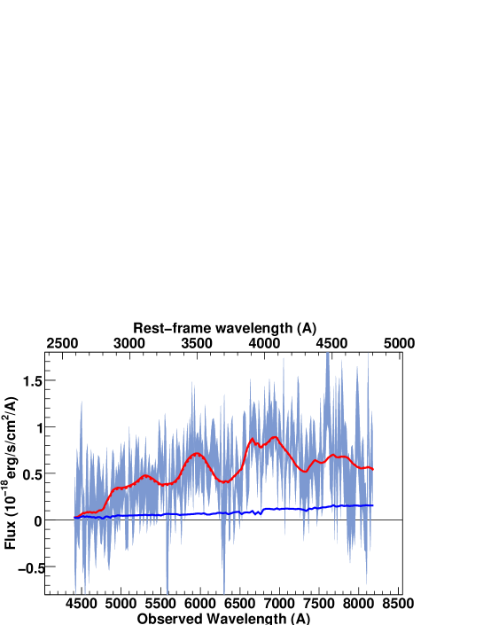
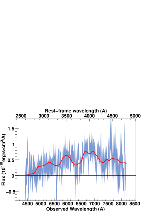
Figure 13: SNLS- 03D1bf269: a SN Ia$\star$ supernova at z=0.703. The spectrum phase is -2.7. A E(3) host model has been subtracted.

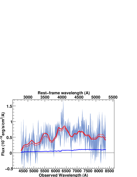
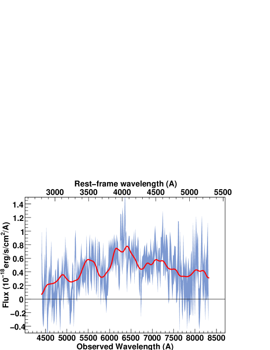
Figure 14: SNLS- 03D1bm272: a SN Ia$\star$ supernova at z=0.575. The spectrum phase is -5.1. A E(3) host model has been subtracted.

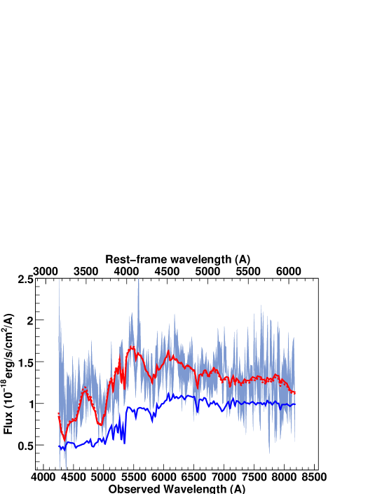
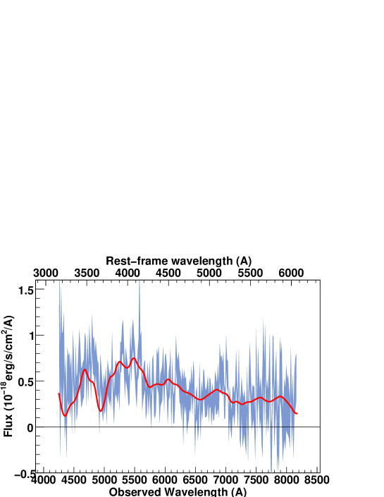
Figure 15: SNLS- 03D1bp270: a SN Ia$\star$ supernova at z=0.347. The spectrum phase is -7.5. A E(2) host model has been subtracted.

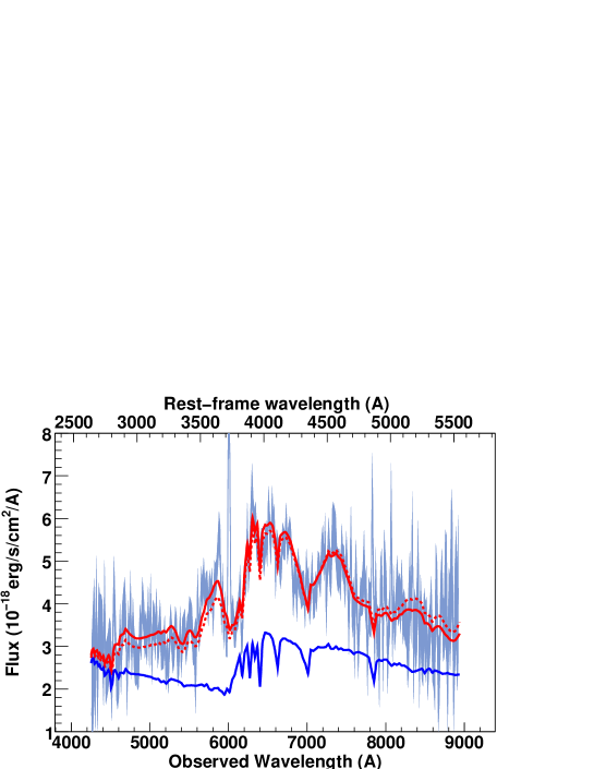
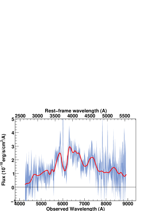
Figure 17: SNLS- 03D1dt333: a SN Ia supernova at z=0.612. The spectrum phase is 5.1. A Sc(4) host model has been subtracted.

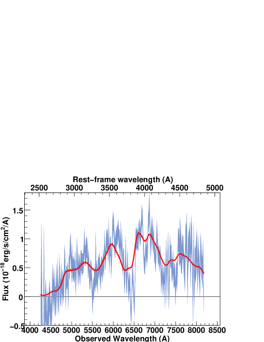
Figure 19: SNLS- 03D1fl355: a SN Ia supernova at z=0.688. The spectrum phase is 0.5. Best-fit obtained for a model with no host galaxy component.

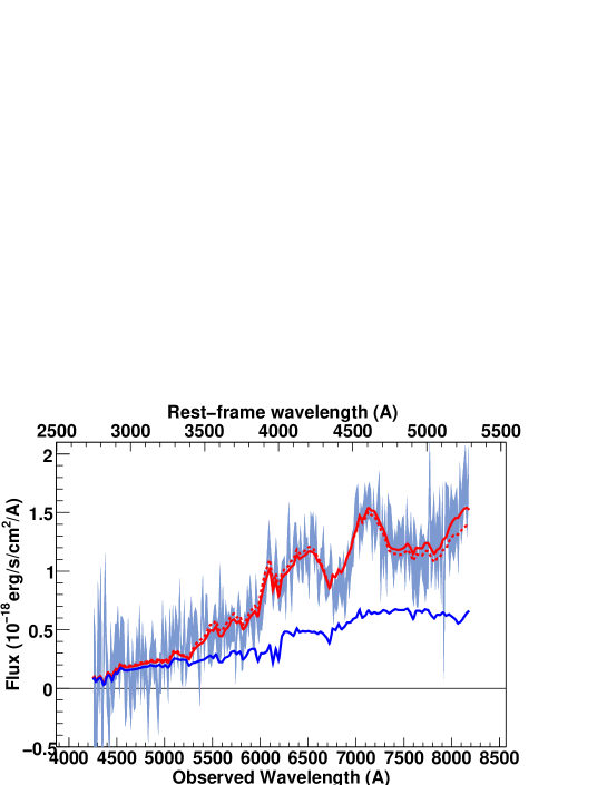
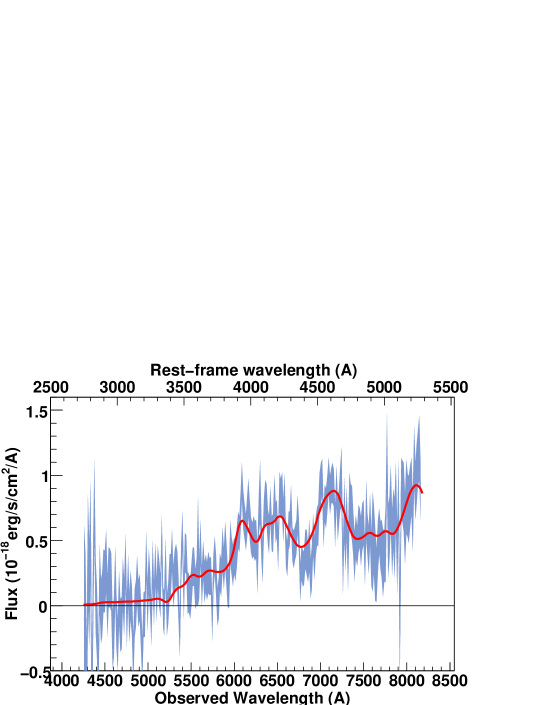
Figure 20: SNLS- 03D1gt385: a SN Ia supernova at z=0.560. The spectrum phase is 7.0. A E(4) host model has been subtracted.

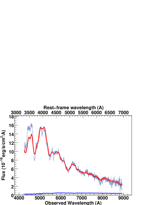
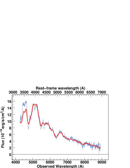
Figure 21: SNLS- 03D4ag180: a SN Ia_pec supernova at z=0.285. The spectrum phase is -8.6. A E(2) host model has been subtracted. Note the poor fit below rest-frame 4000 $\AA$ of this SN 1999aa-like supernova.

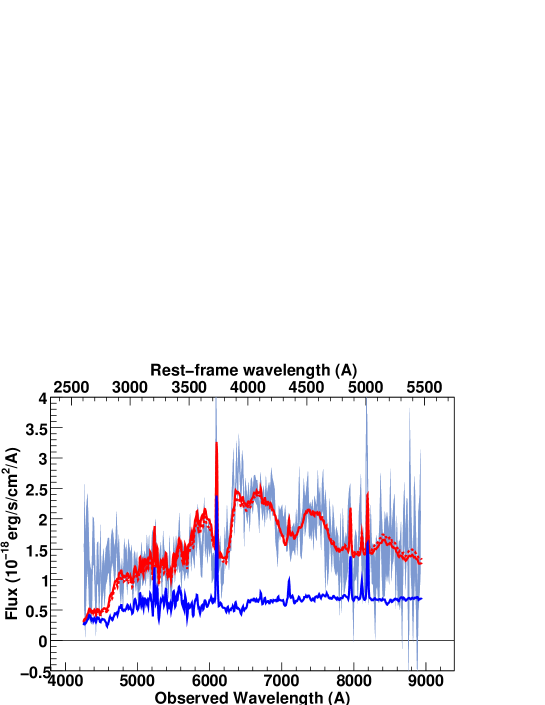
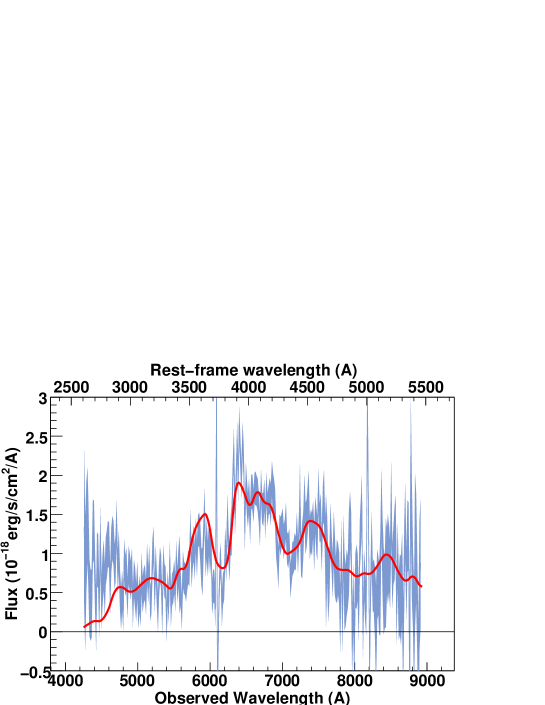
Figure 22: SNLS- 03D4at186: a SN Ia supernova at z=0.634. The spectrum phase is 5.5. A Sb-Sc host model has been subtracted.

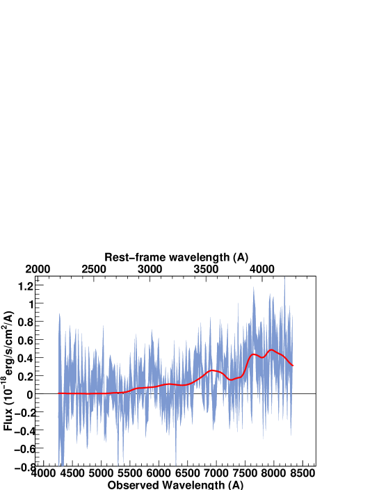
Figure 24: SNLS- 03D4cx245: a SN Ia supernova at z=0.949. The spectrum phase is 1.2. Best-fit obtained for a model with no host galaxy component.

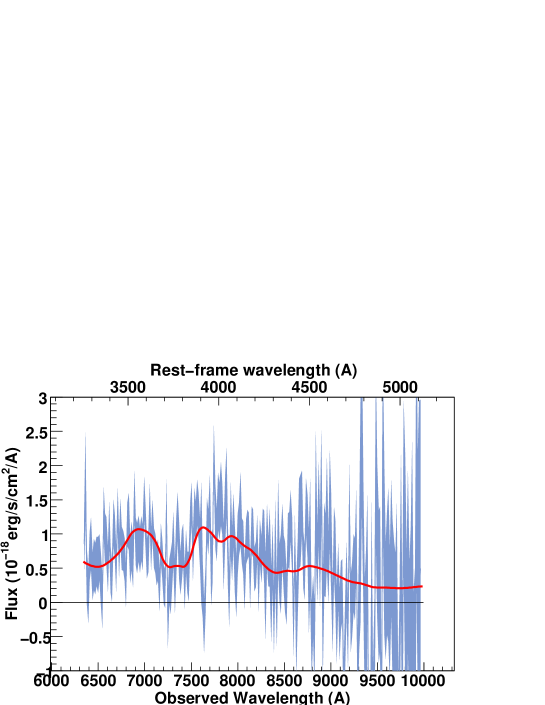
Figure 25: SNLS- 03D4cx248: a SN Ia supernova at z=0.949. Spectrum obtained with the 300I Grism. The spectrum phase is 2.7. A S0(4) host model has been subtracted.

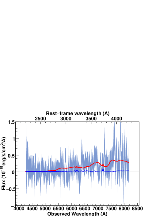
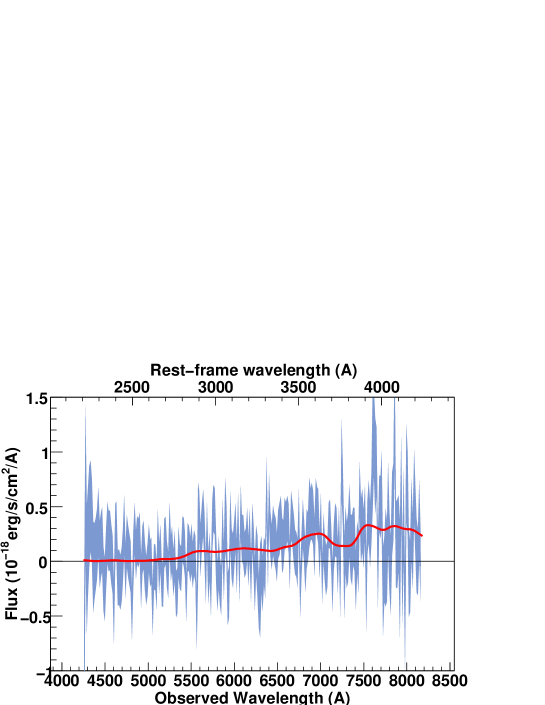
Figure 26: SNLS- 03D4cy269: a SN Ia supernova at z=0.927. The spectrum phase is 4.6. A Sb-Sc host model has been subtracted. The identification of this supernova as a SN Ia is based on a Gemini spectrum of this same SN (Howell et al. 2005)

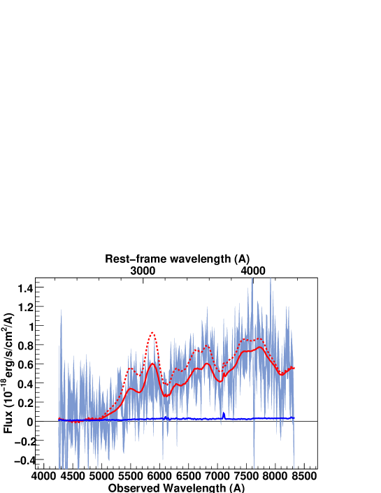
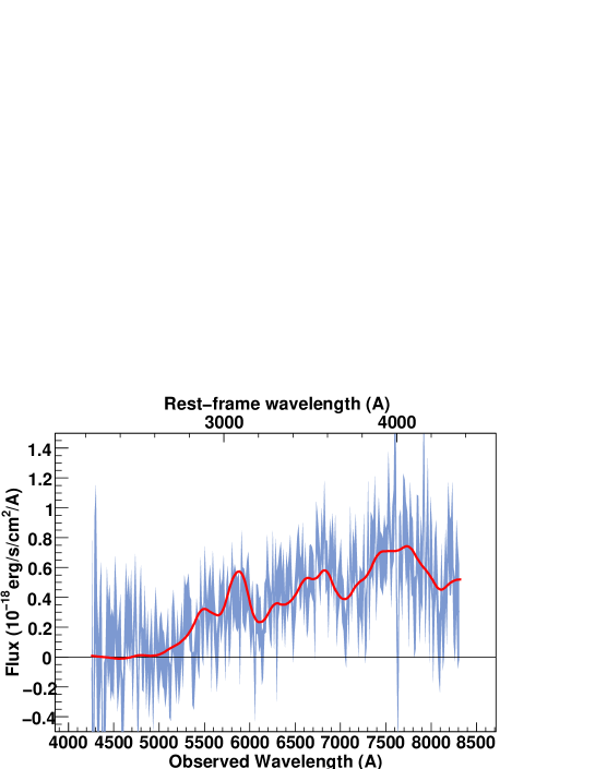
Figure 27: SNLS- 03D4di245: a SN Ia$\star$ supernova at z=0.899. The spectrum phase is -8.6. A Sb-Sc host model has been subtracted.

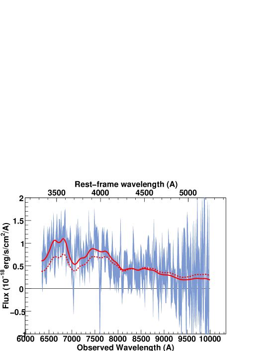
Figure 28: SNLS- 03D4di249: a SN Ia$\star$ supernova at z=0.899. Spectrum obtained with the 300I Grism. The spectrum phase is -6.5. Best-fit obtained for a model with no host galaxy component.

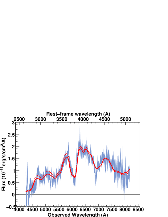
Figure 29: SNLS- 03D4dy272: a SN Ia supernova at z=0.61. The spectrum phase is 4.8. Best-fit obtained for a model with no host galaxy component.

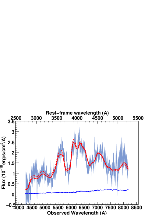
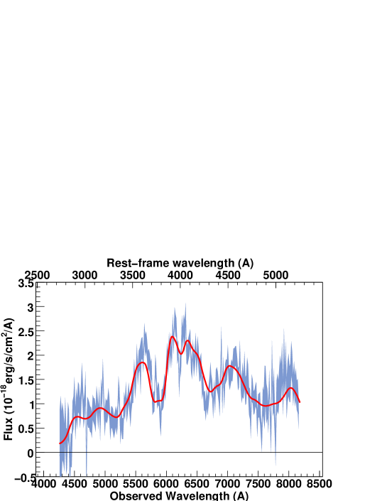
Figure 32: SNLS- 04D1ag383: a SN Ia supernova at z=0.557. The spectrum phase is 4.3. A E(12) host model has been subtracted.

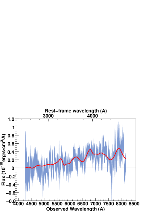
Figure 33: SNLS- 04D1aj381: a SN Ia$\star$ supernova at z=0.721. The spectrum phase is 11.6. Best-fit obtained for a model with no host galaxy component.

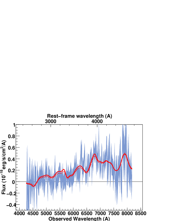
Figure 34: SNLS- 04D1aj384: a SN Ia$\star$ supernova at z=0.721. The spectrum phase is 13.4. Best-fit obtained for a model with no host galaxy component.

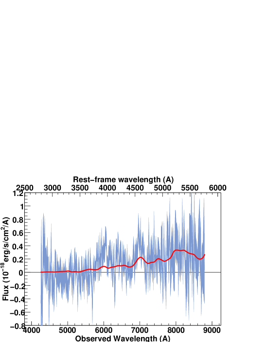
Figure 35: SNLS- 04D1ak388: a SN Ia$\star$ supernova at z=0.526. The spectrum phase is 11.8. Best-fit obtained for a model with no host galaxy component.

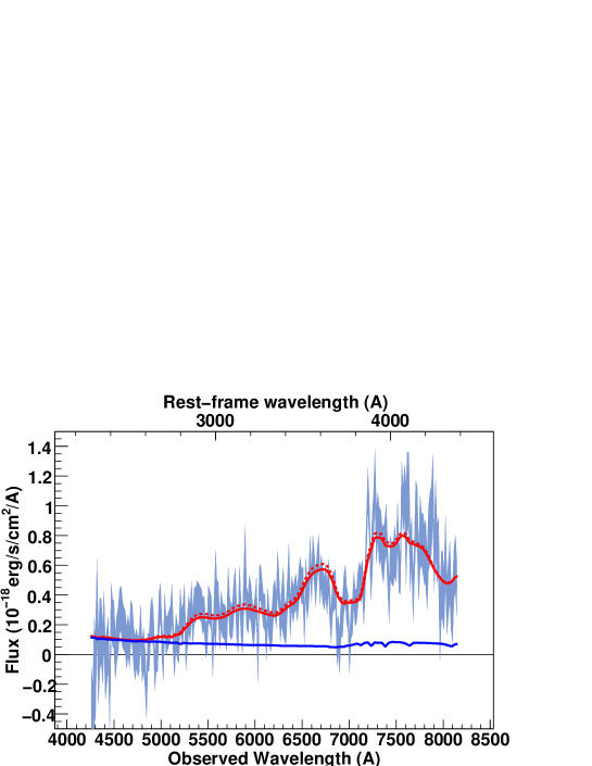
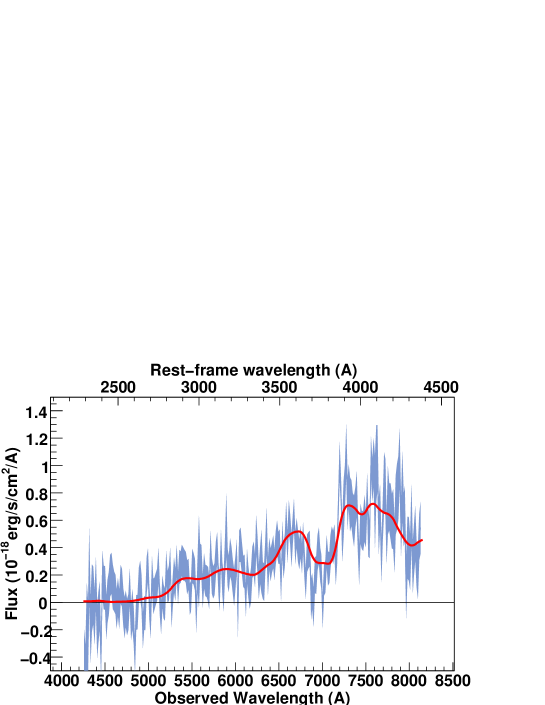
Figure 37: SNLS- 04D1ff619: a SN Ia supernova at z=0.86. The spectrum phase is 4.6. A Sc(2) host model has been subtracted.

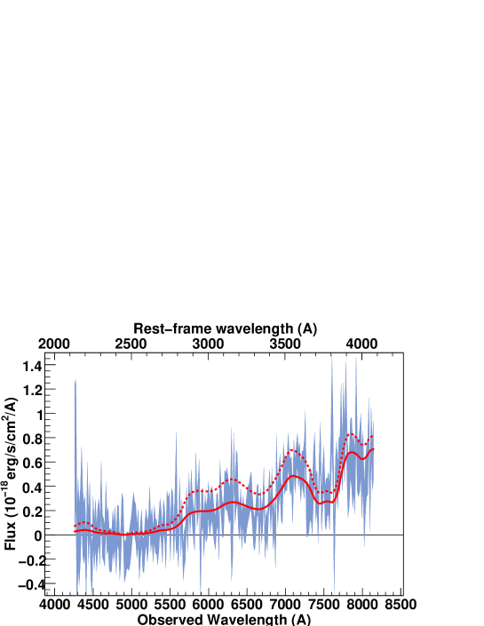
Figure 39: SNLS- 04D1iv630: a SN Ia supernova at z=0.998. The spectrum phase is 3.0. Best-fit obtained for a model with no host galaxy component.

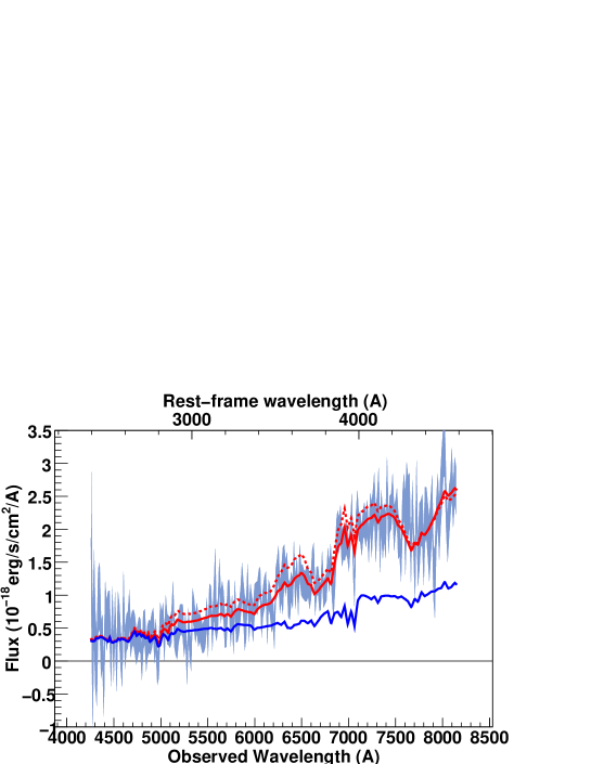
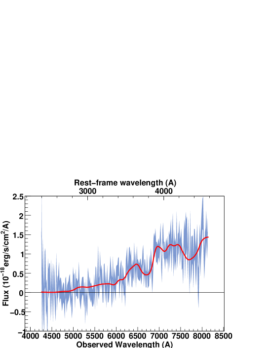
Figure 40: SNLS- 04D1jd630: a SN Ia$\star$ supernova at z=0.778. The spectrum phase is 6.8. A E(2) host model has been subtracted.

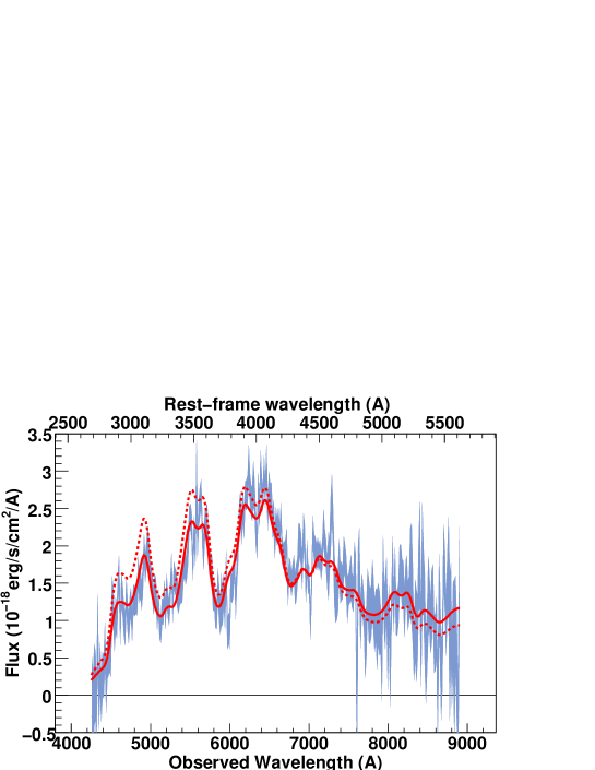
Figure 41: SNLS- 04D1kj650: a SN Ia supernova at z=0.585. The spectrum phase is -3.7. Best-fit obtained for a model with no host galaxy component

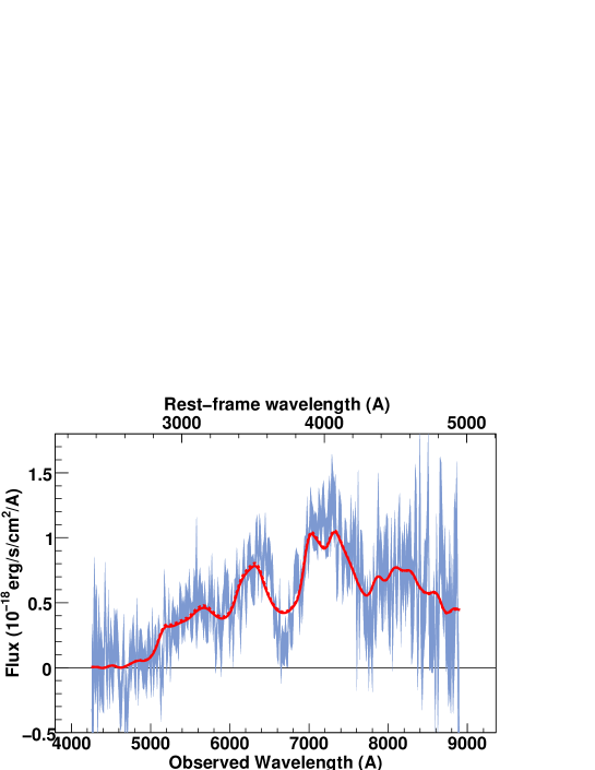
Figure 42: SNLS- 04D1ks649: a SN Ia supernova at z=0.80. The spectrum phase is -1.0. Best-fit obtained for a model with no host galaxy component.

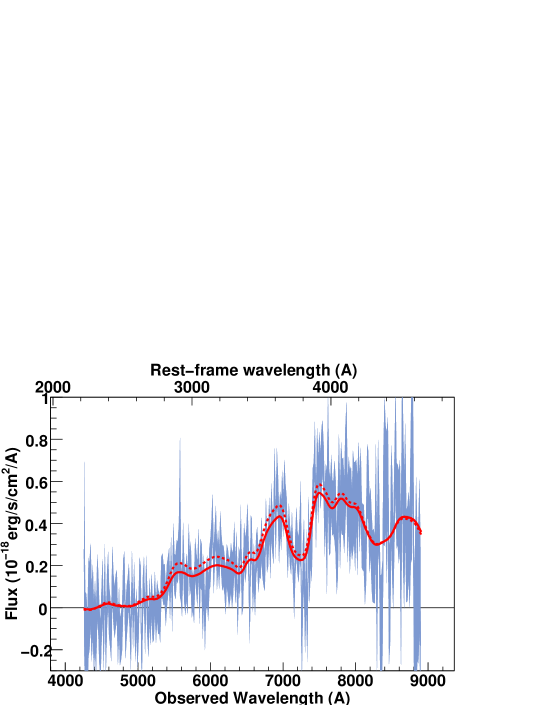
Figure 43: SNLS- 04D1ow683: a SN Ia supernova at z=0.915. The spectrum phase is 6.4. Best-fit obtained for a model with no host galaxy component.

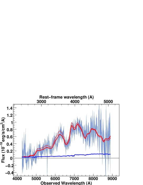
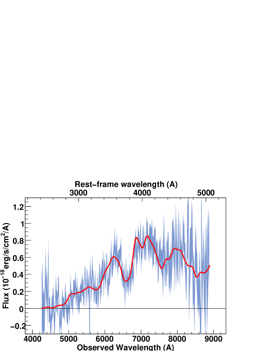
Figure 44: SNLS- 04D1pc684: a SN Ia supernova at z=0.770. The spectrum phase is 0.1. A E(3) host model has been subtracted.

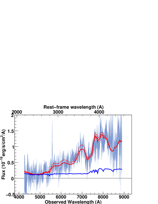
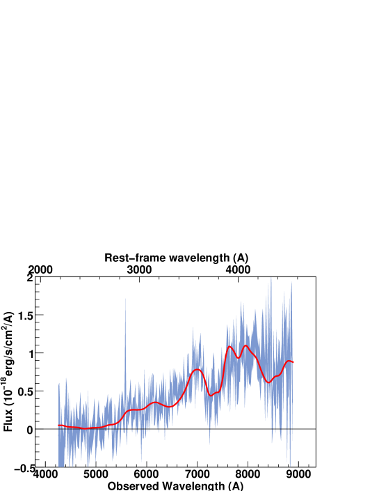
Figure 45: SNLS- 04D1pd682: a SN Ia supernova at z=0.95. The spectrum phase is 2.5. A E(1) host model has been subtracted.

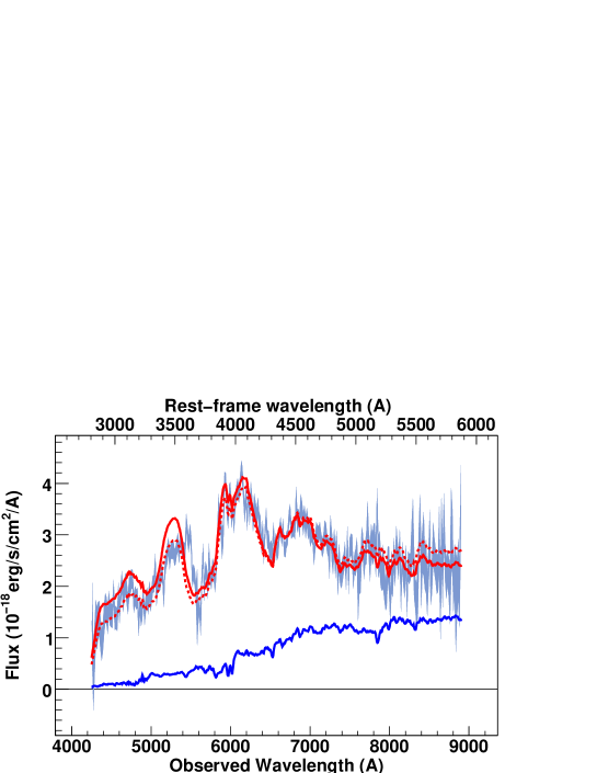
Figure 46: SNLS- 04D1pg684: a SN Ia supernova at z=0.515. The spectrum phase is -1.3. A Sa-Sb host model has been subtracted.

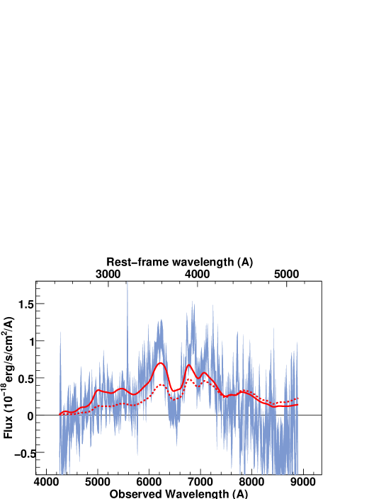
Figure 47: SNLS- 04D1pp683: a SN Ia supernova at z=0.735. The spectrum phase is 2.2. Best-fit obtained for a model with no host galaxy component.

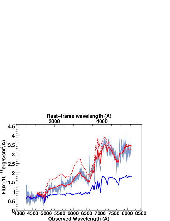
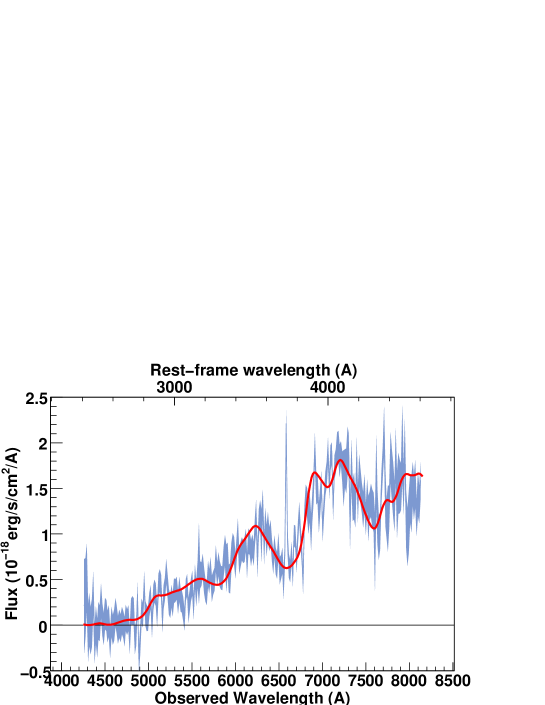
Figure 48: SNLS- 04D1qd688: a SN Ia$\star$ supernova at z=0.767. The spectrum phase is -0.2. A E(1) host model has been subtracted.

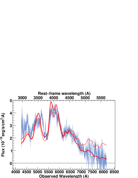
Figure 49: SNLS- 04D1rh710: a SN Ia supernova at z=0.436. The spectrum phase is 0.0. Best-fit obtained for a model with no host galaxy.

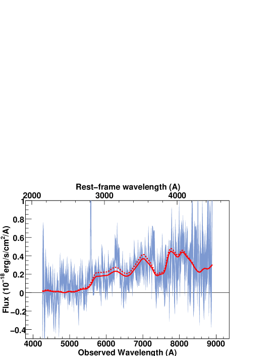
Figure 50: SNLS- 04D1rx713: a SN Ia$\star$ supernova at z=0.985. The spectrum phase is 0.9. Best-fit obtained for a model with no host galaxy component.

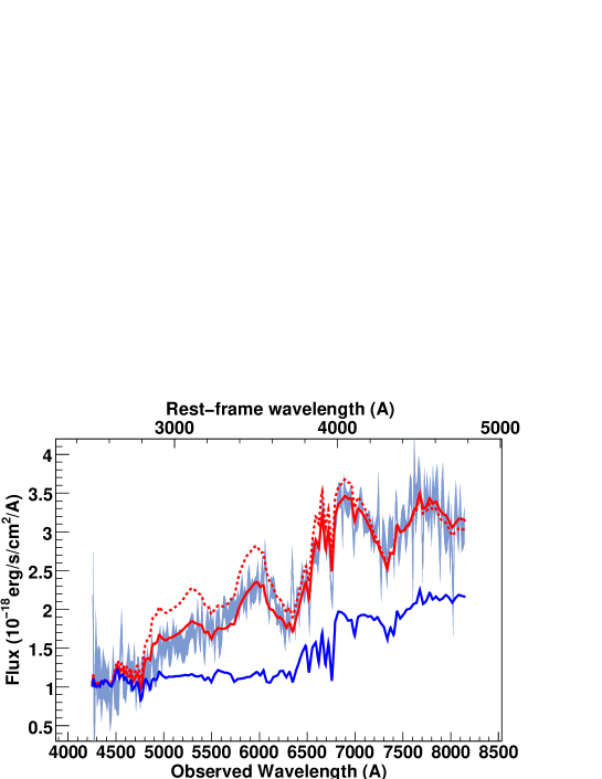
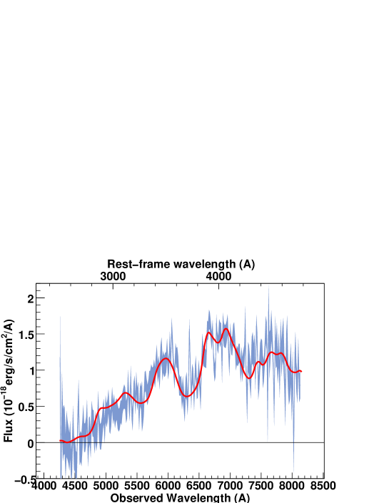
Figure 52: SNLS- 04D1si716: a SN Ia supernova at z=0.702. The spectrum phase is -1.7. A Sa(9) host model has been subtracted.

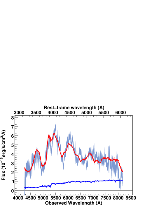
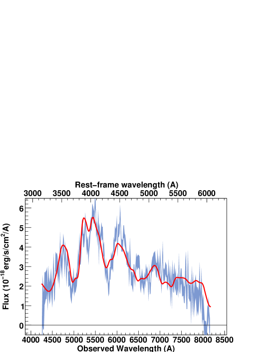
Figure 53: SNLS- 04D2ac395: a SN Ia supernova at z=0.348. The spectrum phase is 1.3. A Sa-Sb host model has been subtracted.

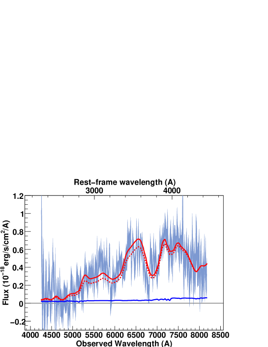
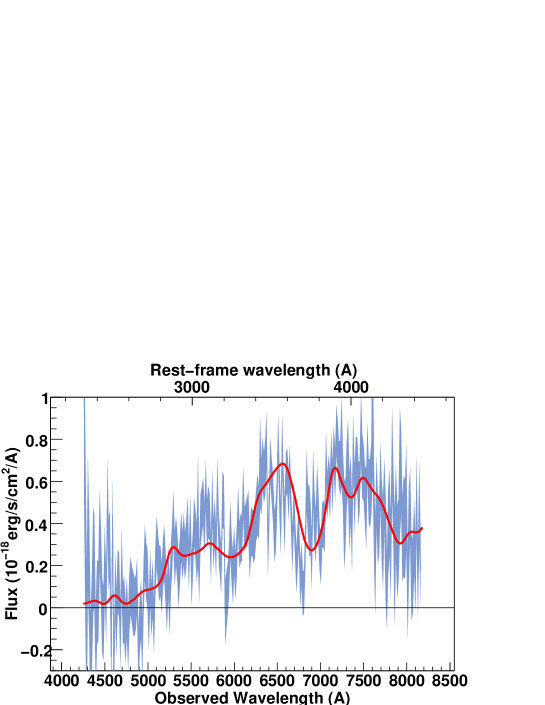
Figure 54: SNLS- 04D2al390: a SN Ia supernova at z=0.836. The spectrum phase is -2.5. A E(2) host model has been subtracted.

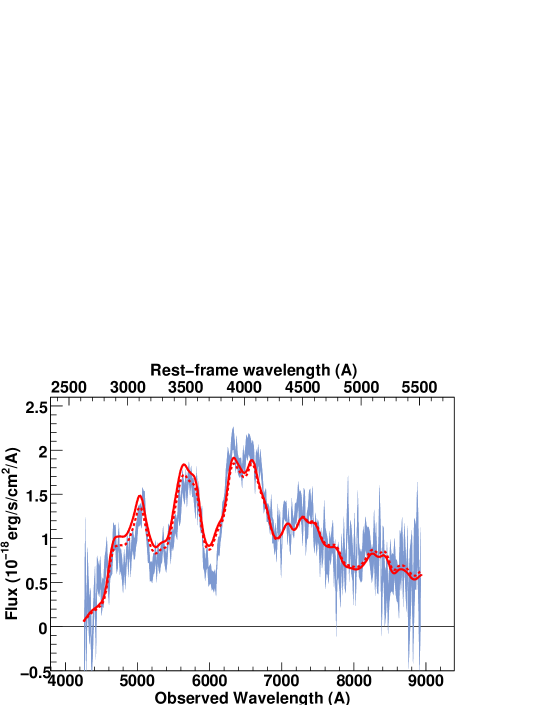
Figure 55: SNLS- 04D2an386: a SN Ia supernova at z=0.62. The spectrum phase is -3.4. Best-fit obtained for a model with no host galaxy component. Note that the Ca ii feature at rest-frame 3700 $\AA$ is deeper than in the model.

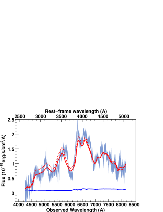
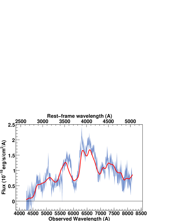
Figure 56: SNLS- 04D2an392: a SN Ia supernova at z=0.62. The spectrum phase is 0.3. A Sc(9) host model has been subtracted.

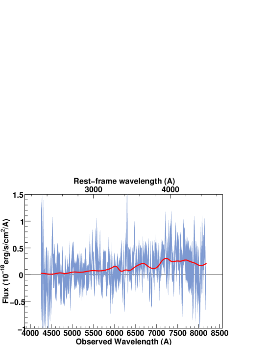
Figure 58: SNLS- 04D2ca445: a SN Ia$\star$ supernova at z=0.835. The spectrum phase is 12.0. Best-fit obtained for a model with no host galaxy component.

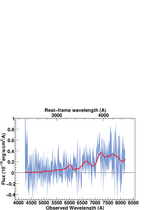
Figure 59: SNLS- 04D2ca447: a SN Ia$\star$ supernova at z=0.835. The spectrum phase is 13.1. Best-fit obtained for a model with no host galaxy component.

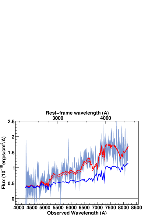
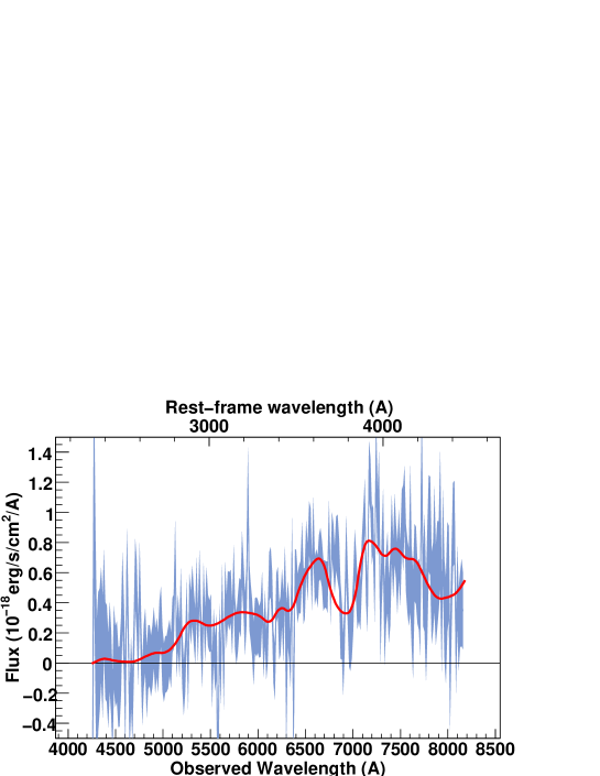
Figure 60: SNLS- 04D2cc446: a SN Ia$\star$ supernova at z=0.838. The spectrum phase is 6.1. A S0(3) host model has been subtracted.

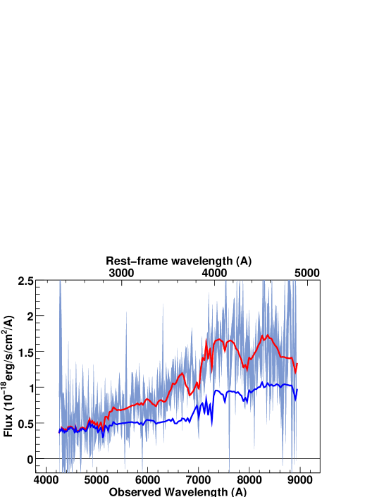
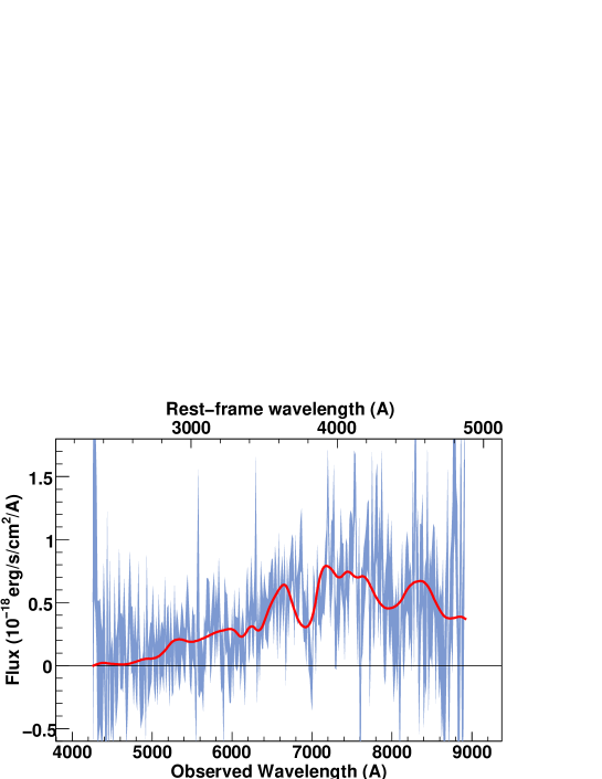
Figure 61: SNLS- 04D2cc448: a SN Ia$\star$ supernova at z=0.838. The spectrum phase is 7.2. A S0(2) host model has been subtracted.

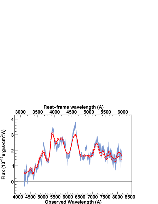
Figure 62: SNLS- 04D2cf447: a SN Ia supernova at z=0.369. The spectrum phase is 8.5. Best-fit obtained for a model with no host galaxy component. Note that the model is unable to reproduce the feature at rest-frame 4900 $\AA$.

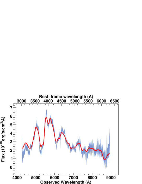
Figure 64: SNLS- 04D2fp470: a SN Ia supernova at z=0.415. The spectrum phase is 1.8. Best-fit obtained for a model with no host galaxy component.

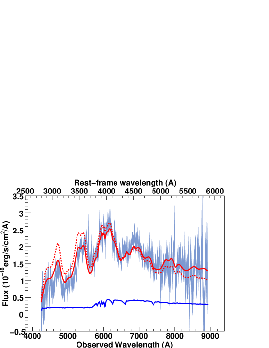
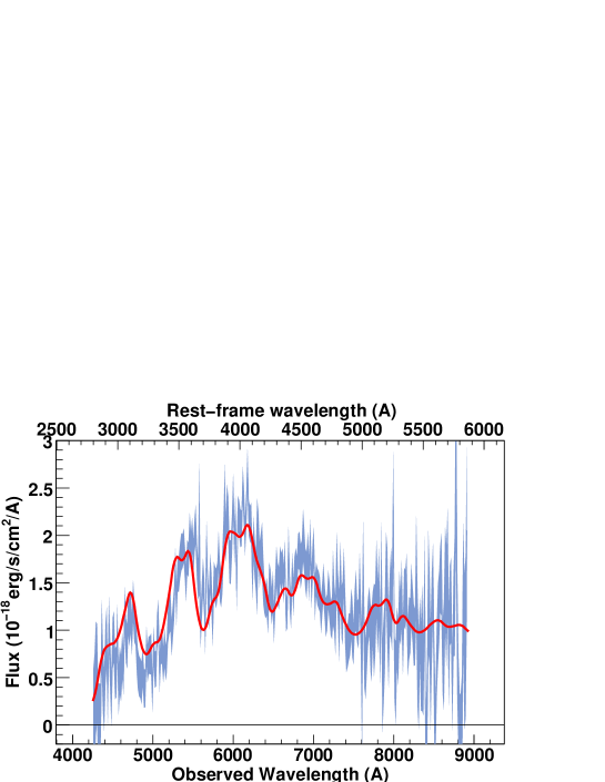
Figure 66: SNLS- 04D2gc471: a SN Ia supernova at z=0.521. The spectrum phase is -4.9. A E(1) host model has been subtracted.

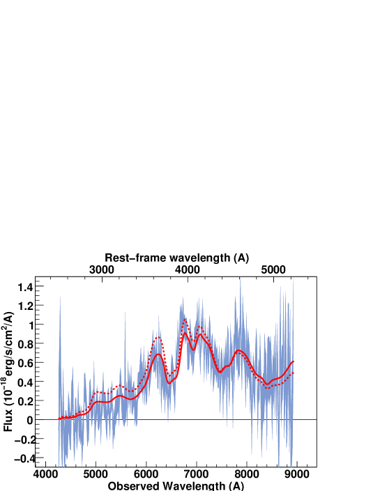
Figure 67: SNLS- 04D2gp475: a SN Ia supernova at z=0.732. The spectrum phase is 2.7. Best-fit obtained for a model with no host galaxy component.

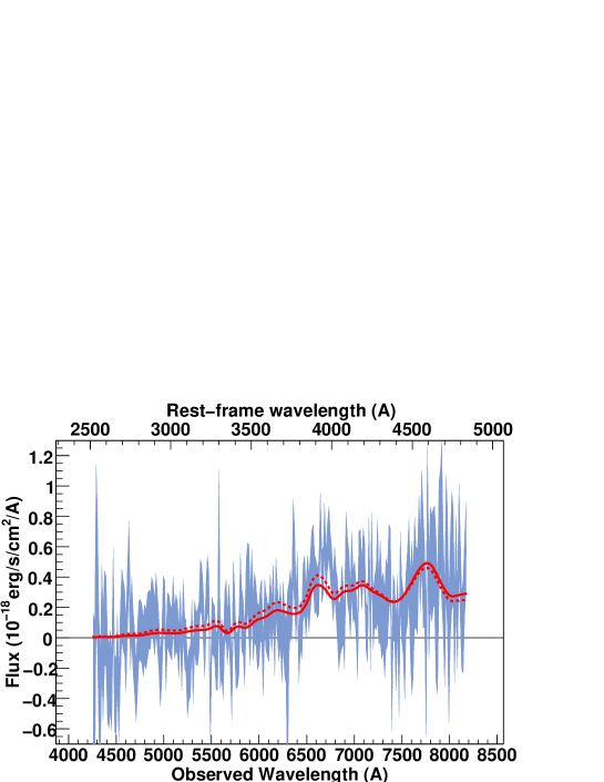
Figure 68: SNLS- 04D2iu497: a SN Ia$\star$ supernova at z=0.70. The spectrum phase is 9.8. Best-fit obtained for a model with no host galaxy component.

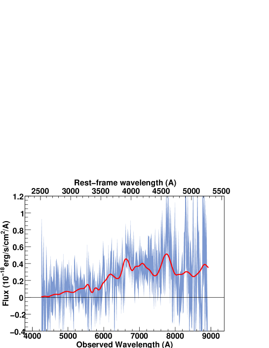
Figure 69: SNLS- 04D2iu498: a SN Ia$\star$ supernova at z=0.70. The spectrum phase is 10.4. A E(1) host model has been subtracted.

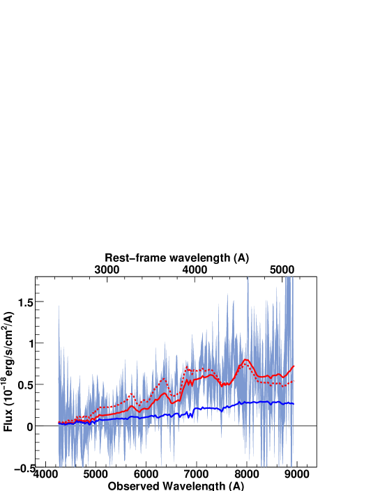
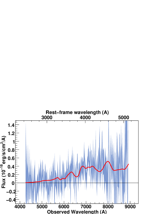
Figure 70: SNLS- 04D2ja499: a SN Ia$\star$ supernova at z=0.740. The spectrum phase is 9.2. A E(3) host model has been subtracted. Note the large feature at rest-frame 4800 $\AA$ not reproduced by the model.

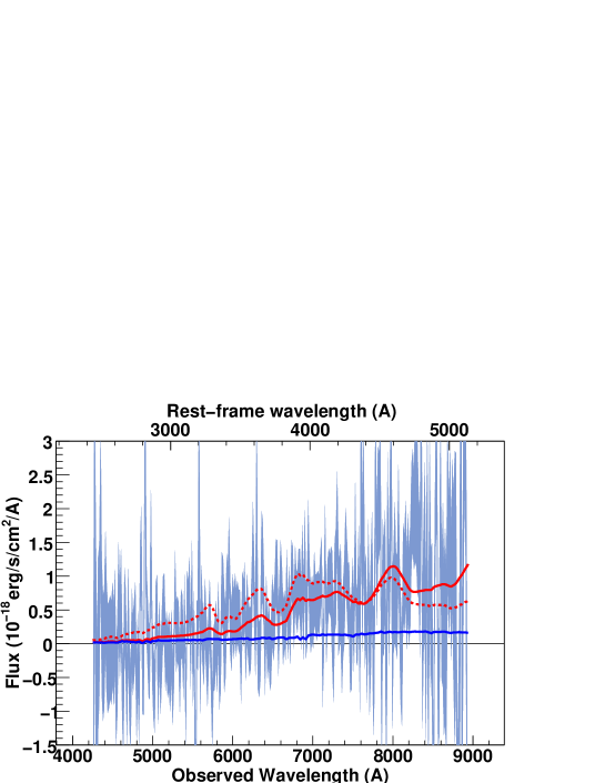
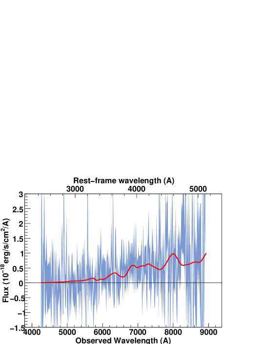
Figure 71: SNLS- 04D2ja500: a SN Ia$\star$ supernova at z=0.740. The spectrum phase is 9.8. A E(3) host model has been subtracted.

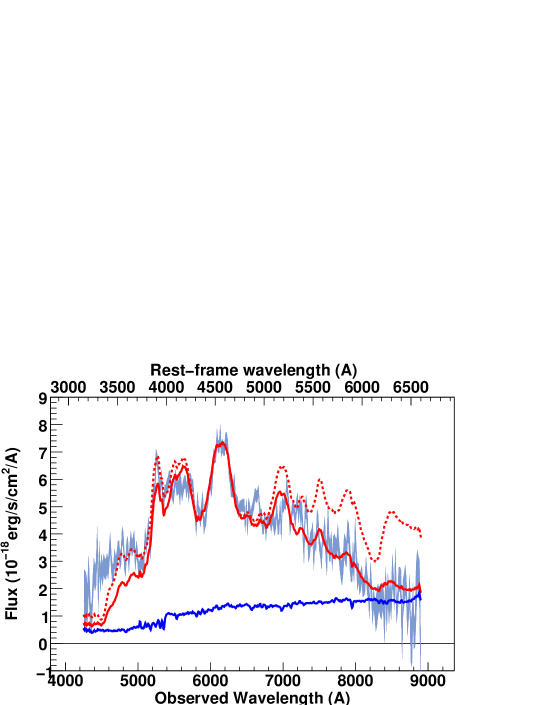
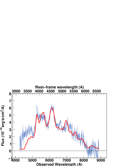
Figure 72: SNLS- 04D2mc736: a SN Ia supernova at z=0.348. The spectrum phase is 6.5. A Sa-Sb host model has been subtracted. Three re-calibration parameters have been used to fit this spectrum.

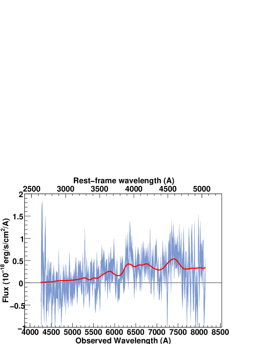
Figure 73: SNLS- 04D4an558: a SN Ia supernova at z=0.613. The spectrum phase is 8.1. Best-fit obtained for a model with no host galaxy component.

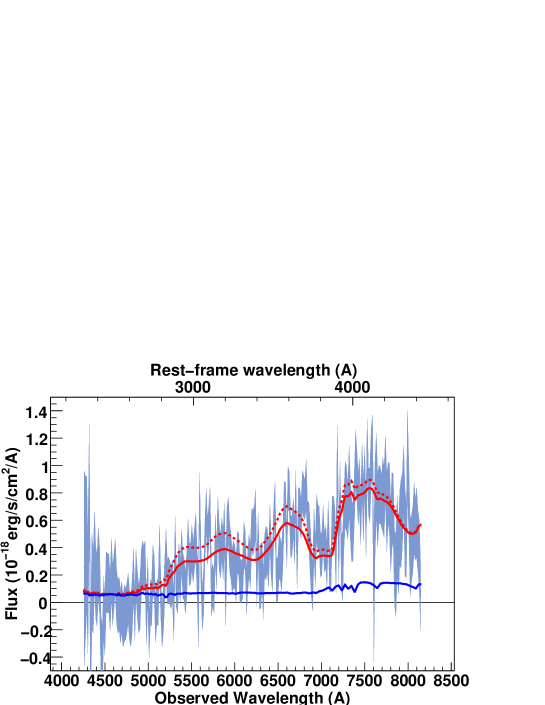
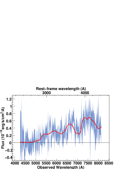
Figure 74: SNLS- 04D4bk558: a SN Ia$\star$ supernova at z=0.88. The spectrum phase is 3.1. A E(1) host model has been subtracted.

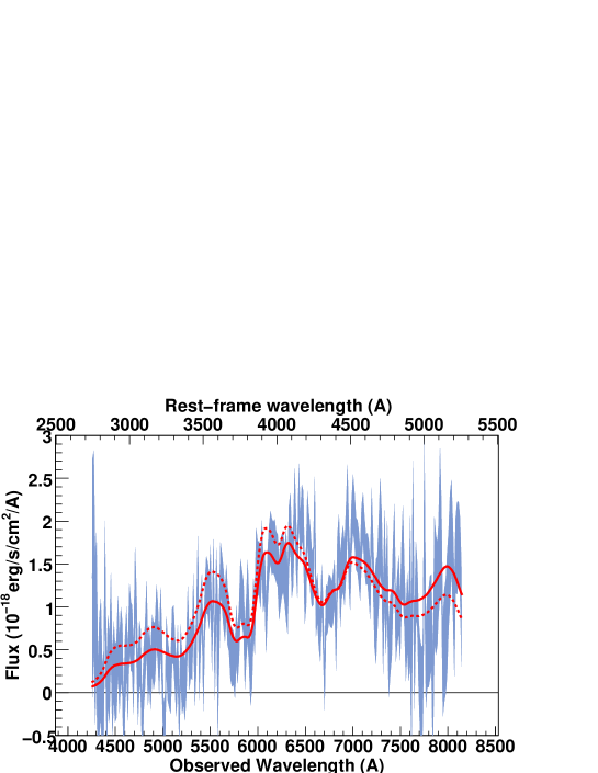
Figure 75: SNLS- 04D4bq558: a SN Ia supernova at z=0.55. The spectrum phase is 2.6. Best-fit obtained for a model with no host galaxy component.

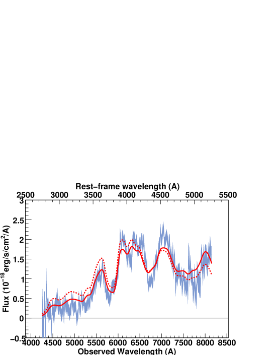
Figure 76: SNLS- 04D4bq562: a SN Ia supernova at z=0.55. The spectrum phase is 5.1. Best-fit obtained for a model with no host galaxy component.

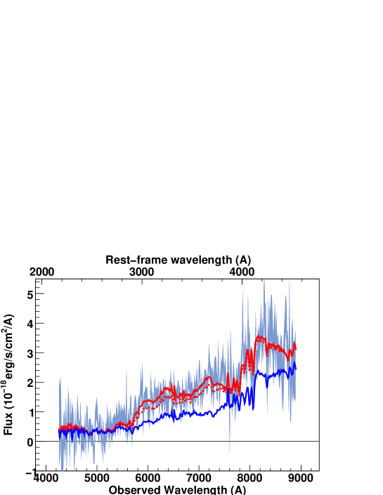
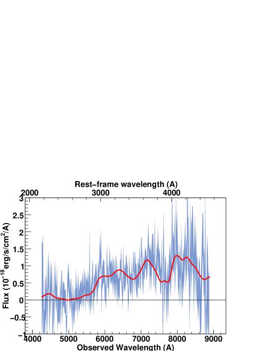
Figure 77: SNLS- 04D4dw566: a SN Ia$\star$ supernova at z=1.031. The spectrum phase is 2.1. A Sa-Sb host model has been subtracted.

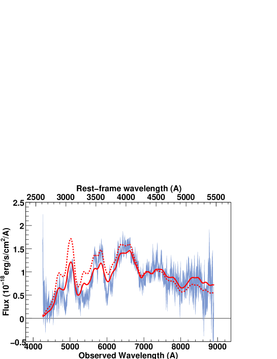
Figure 78: SNLS- 04D4fx589: a SN Ia supernova at z=0.629. The spectrum phase is -8.4. Best-fit obtained for a model with no host galaxy component.

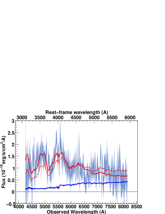
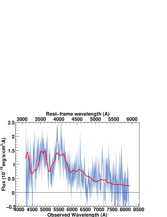
Figure 79: SNLS- 04D4gz598: a SN Ia$\star$ supernova at z=0.375. The spectrum phase is -5.8. A Sa-Sb host model has been subtracted.

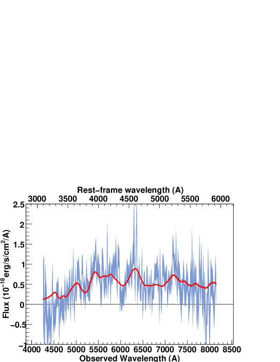
Figure 80: SNLS- 04D4gz620: a SN Ia$\star$ supernova at z=0.375. The spectrum phase is 10.2. Best-fit obtained for a model with no host galaxy component.

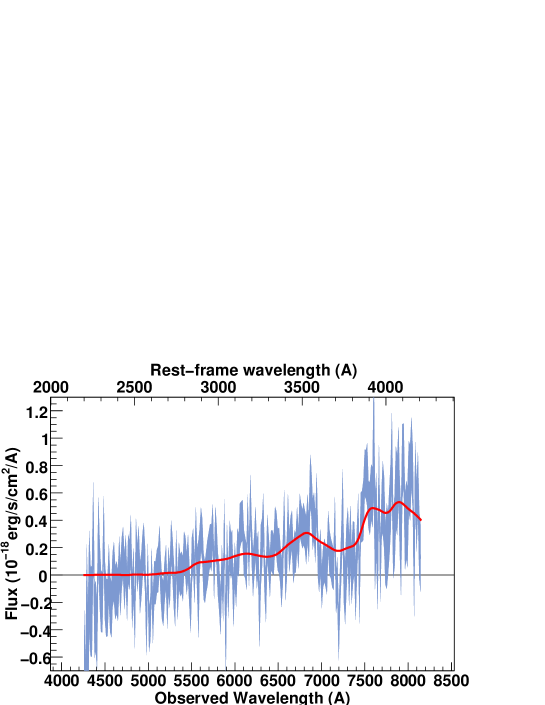
Figure 81: SNLS- 04D4hf598: a SN Ia$\star$ supernova at z=0.94. The spectrum phase is -0.5. Best-fit obtained for a model with no host galaxy component.

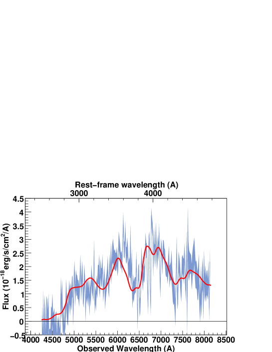
Figure 83: SNLS- 04D4ib629: a SN Ia supernova at z=0.699. The spectrum phase is 0.7. A S0-Sa host model has been subtracted.

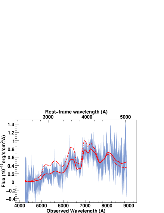
Figure 84: SNLS- 04D4id628: a SN Ia supernova at z=0.769. The spectrum phase is 3.0. Best-fit obtained for a model with no host galaxy component.

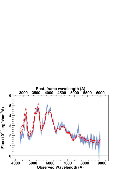
Figure 85: SNLS- 04D4jr650: a SN Ia supernova at z=0.47. The spectrum phase is -5.9. Best-fit obtained for a model with no host galaxy component.

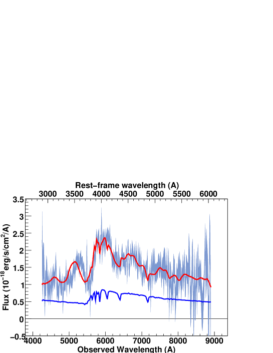
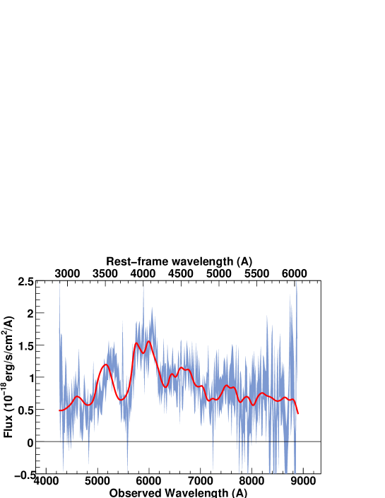
Figure 86: SNLS- 04D4ju650: a SN Ia supernova at z=0.472. The spectrum phase is -2.2. A S0(1) host model has been subtracted.

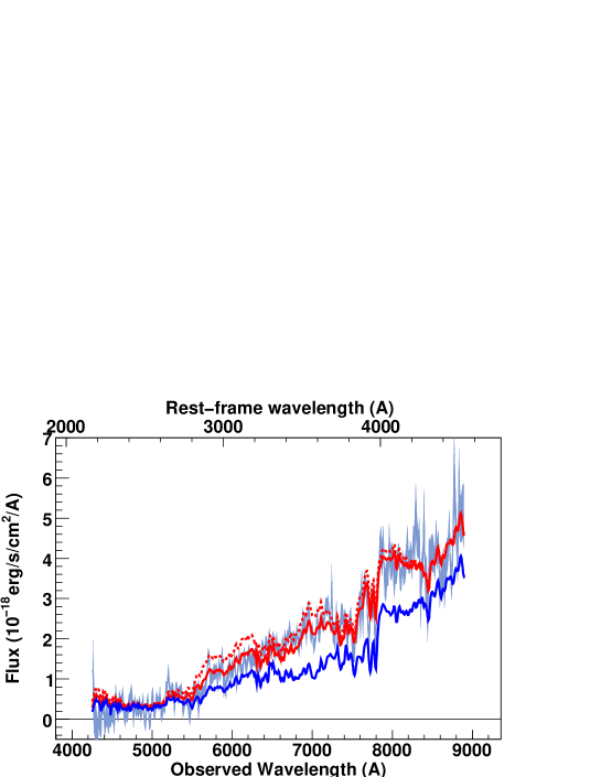
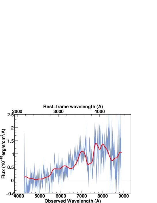
Figure 87: SNLS- 04D4jw651: a SN Ia$\star$ supernova at z=0.961. The spectrum phase is 2.2. A S0-Sa host model has been subtracted.

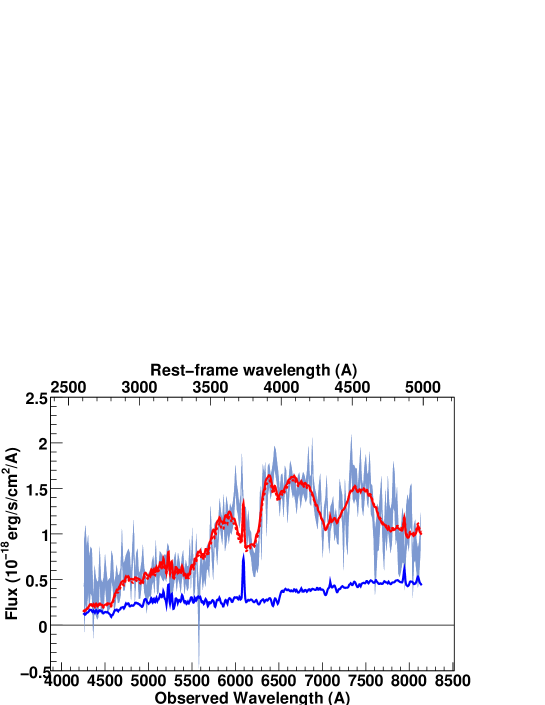
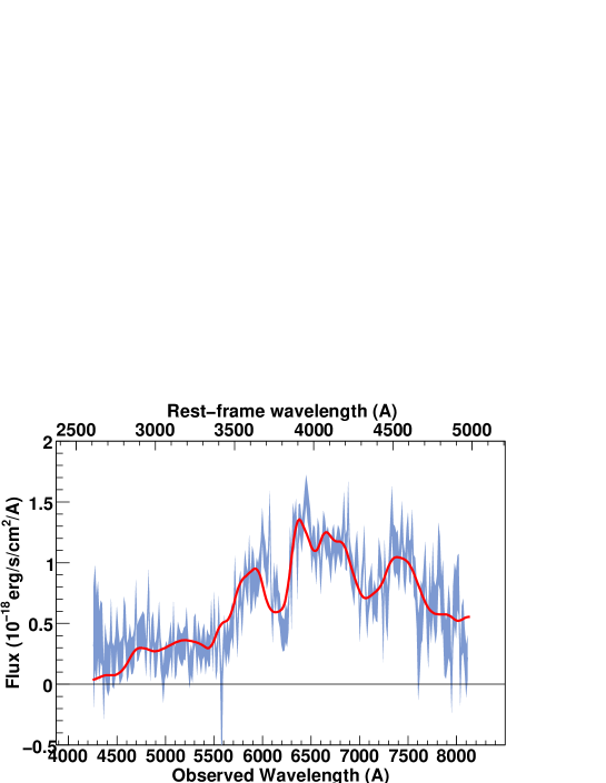
Figure 88: SNLS- 05D1cb984: a SN Ia supernova at z=0.632. The spectrum phase is 4.3. A Sb-Sc host model has been subtracted.

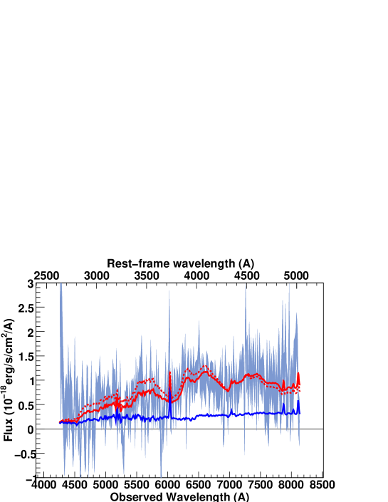
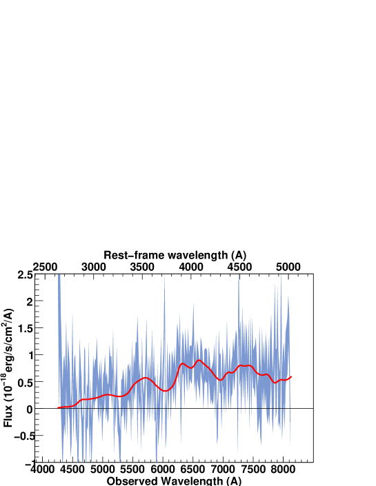
Figure 89: SNLS- 05D1ck983: a SN Ia supernova at z=0.617. The spectrum phase is -2.7. A Sb-Sc host model has been subtracted.

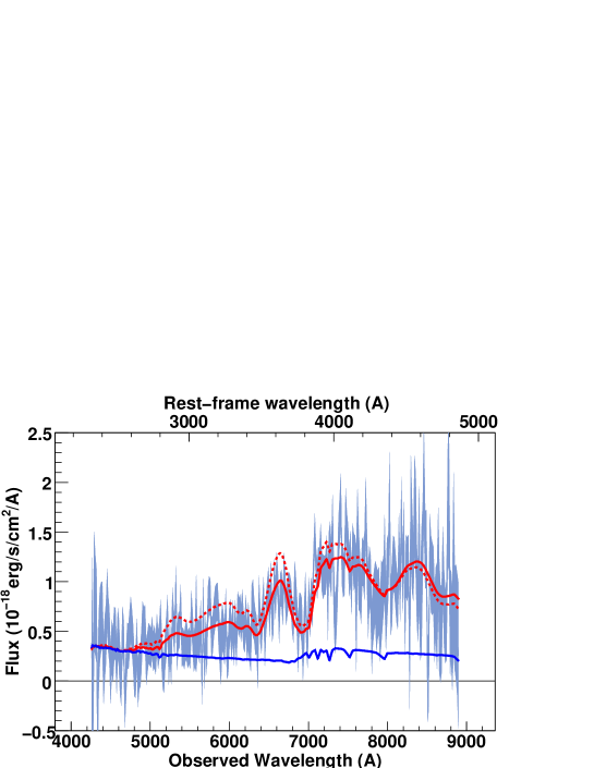
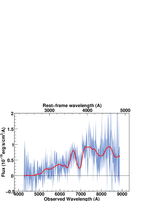
Figure 90: SNLS- 05D1cl999: a SN Ia$\star$ supernova at z=0.83. The spectrum phase is 8.7. A Sd(4) host model has been subtracted.

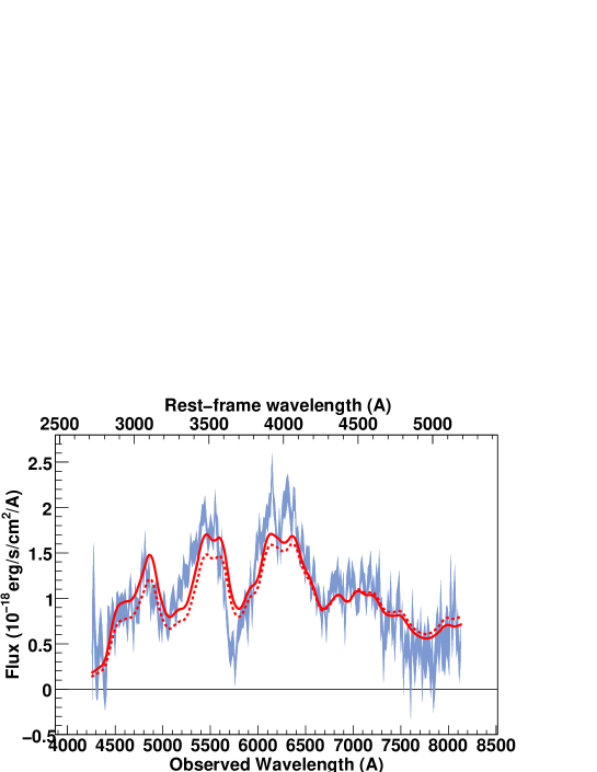
Figure 91: SNLS- 05D1dn1002: a SN Ia supernova at z=0.566. The spectrum phase is -4.7. Best-fit obtained for a model with no host galaxy component.

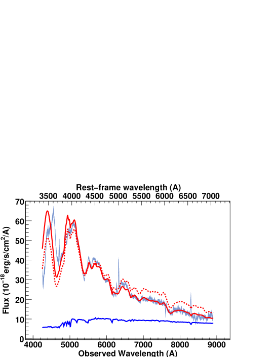
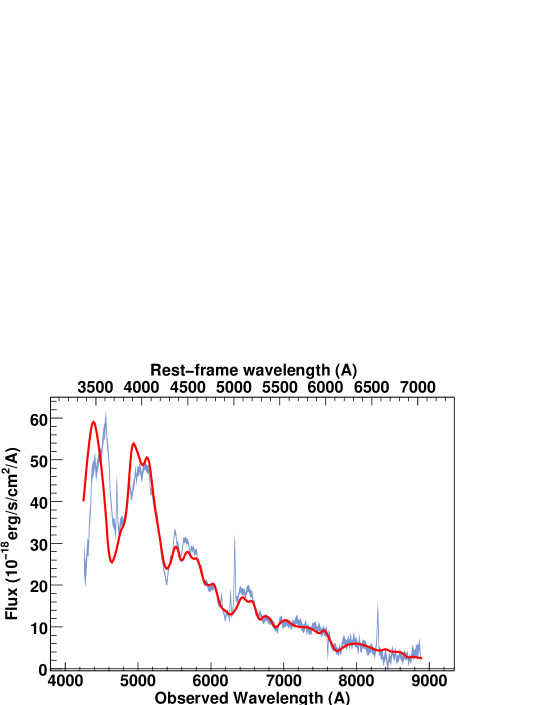
Figure 92: SNLS- 05D1hk1072: a SN Ia_pec supernova at z=0.263. The spectrum phase is -5.0. A Sc(5) host model has been subtracted.

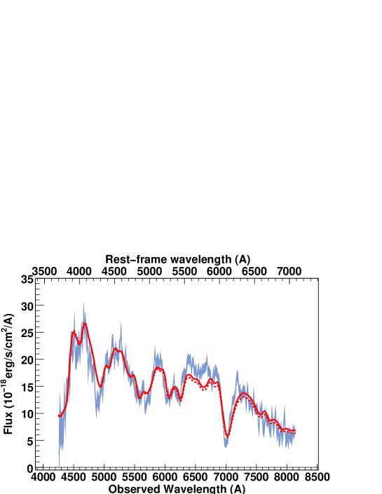
Figure 93: SNLS- 05D1hn1073: a SN Ia supernova at z=0.149. The spectrum phase is -1.0. Best-fit obtained for a model with no host galaxy component. This is a very reddened SN Ia due to host interstellar absorption.

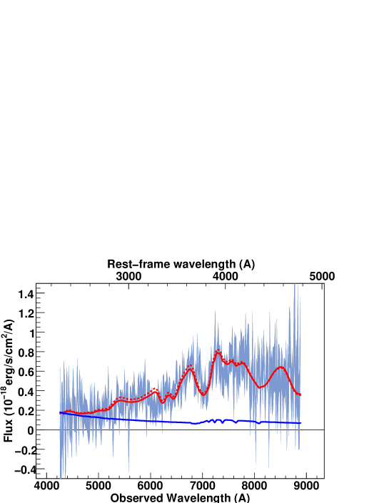
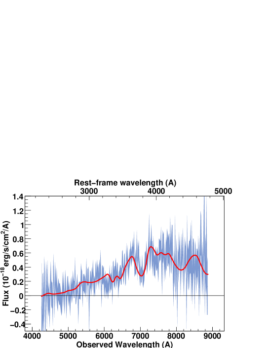
Figure 94: SNLS- 05D1iz1069: a SN Ia$\star$ supernova at z=0.86. The spectrum phase is 7.8. A Sd(1) host model has been subtracted.

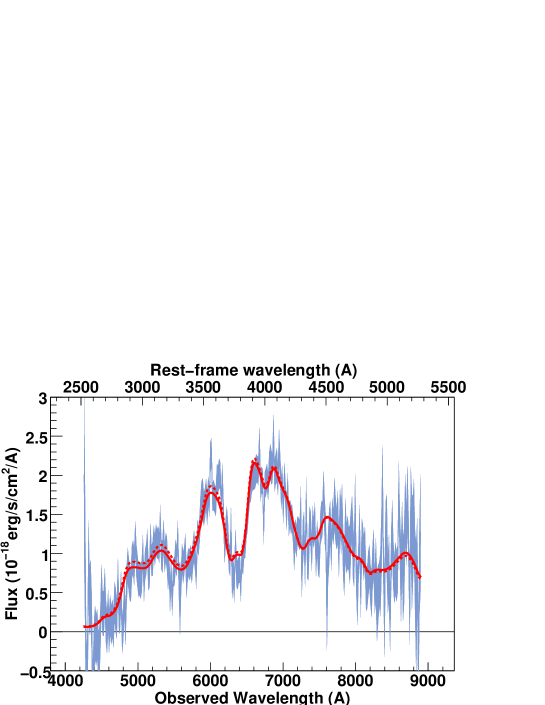
Figure 95: SNLS- 05D1ke1094: a SN Ia supernova at z=0.69. The spectrum phase is 2.2. Best-fit obtained for a model with no host galaxy component.

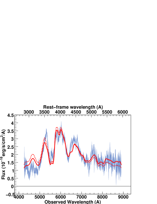
Figure 96: SNLS- 05D2ac738: a SN Ia supernova at z=0.479. The spectrum phase is 2.0. Best-fit obtained for a model with no host galaxy component. Note that the model overestimates the flux in the UV region of the spectrum.

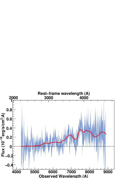
Figure 97: SNLS- 05D2ay746: a SN Ia$\star$ supernova at z=0.92. The spectrum phase is 5.8. A S0(1) host model has been subtracted.

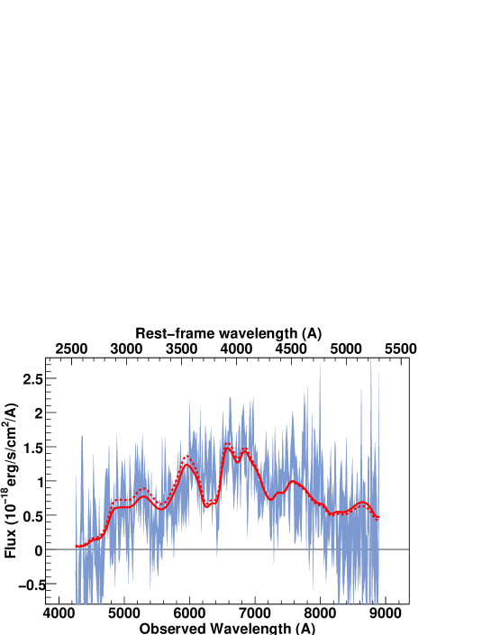
Figure 98: SNLS- 05D2bt764: a SN Ia supernova at z=0.68. The spectrum phase is 1.4. Best-fit obtained for a model with no host galaxy component.

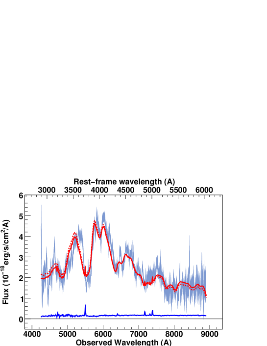
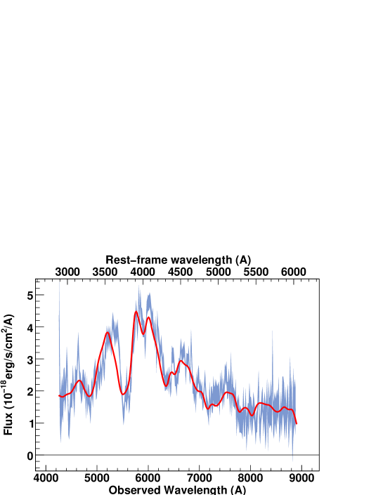
Figure 99: SNLS- 05D2bv764: a SN Ia supernova at z=0.474. The spectrum phase is -0.1. A Sb-Sc host model has been subtracted. Note that the Ca ii feature at rest-frame 3700 $\AA$ is narrower than in the model.

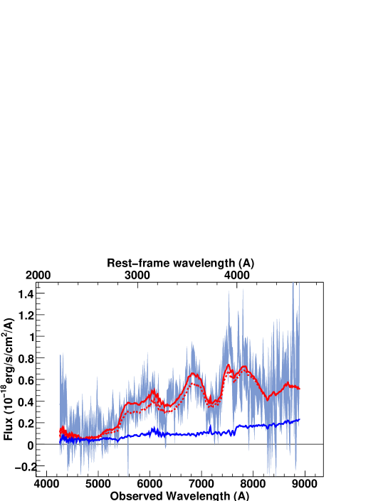
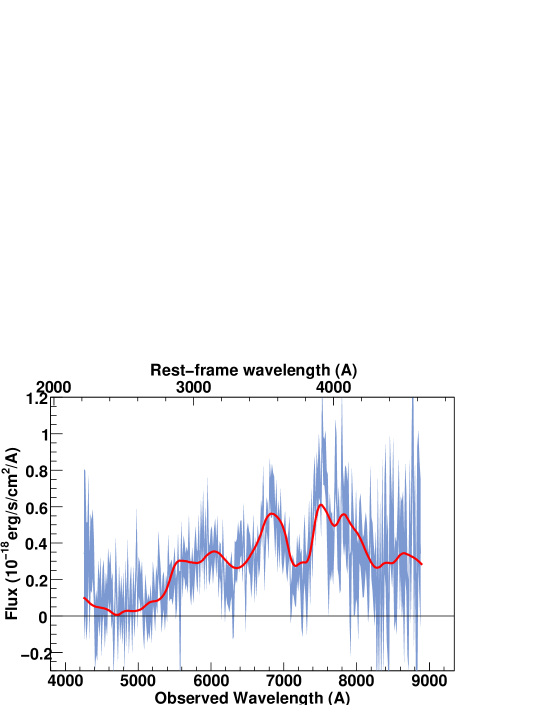
Figure 100: SNLS- 05D2bw764: a SN Ia supernova at z=0.92. The spectrum phase is 1.9. A Sb-Sc host model has been subtracted.

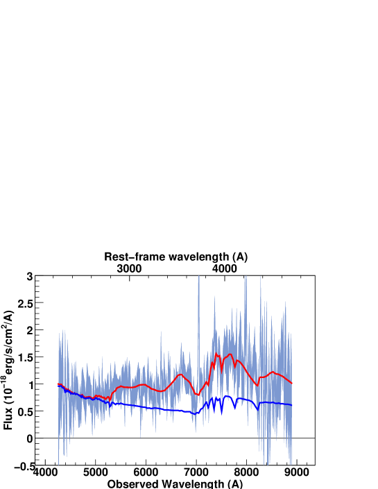
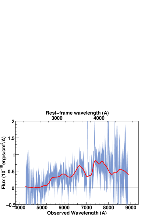
Figure 101: SNLS- 05D2by775: a SN Ia$\star$ supernova at z=0.891. The spectrum phase is 0.9. A Sc(11) host model has been subtracted.

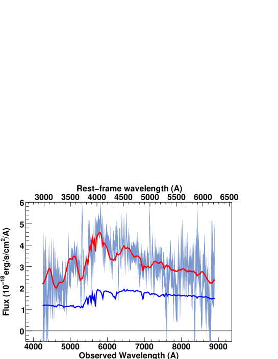
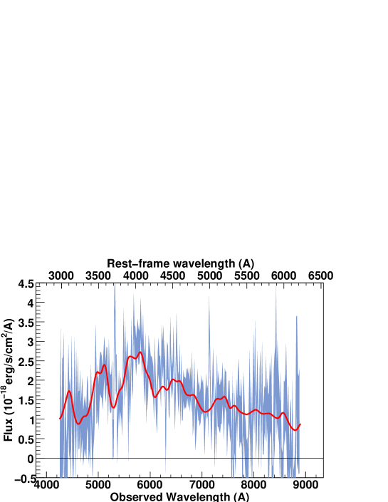
Figure 102: SNLS- 05D2cb775: a SN Ia$\star$ supernova at z=0.427. The spectrum phase is -5.8. A Sc(11) host model has been subtracted.

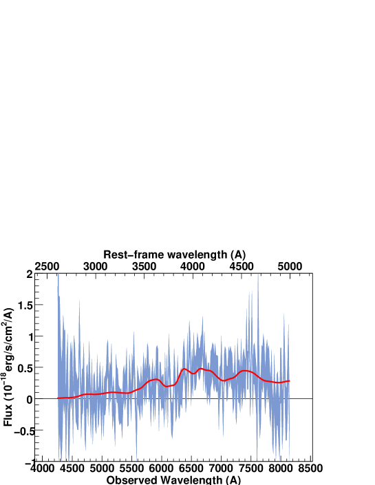
Figure 103: SNLS- 05D2ci795: a SN Ia supernova at z=0.630. The spectrum phase is 3.6. Best-fit obtained for a model with no host galaxy component.

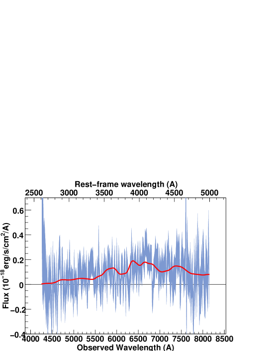
Figure 104: SNLS- 05D2ci796: a SN Ia supernova at z=0.630. The spectrum phase is 4.9. Best-fit obtained for a model with no host galaxy component.

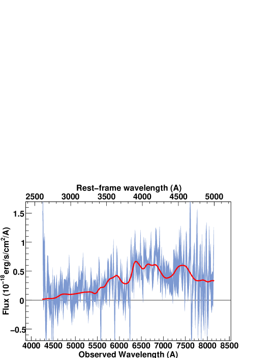
Figure 105: SNLS- 05D2ci799: a SN Ia supernova at z=0.630. The spectrum phase is 6.7. Best-fit obtained for a model with no host galaxy component.

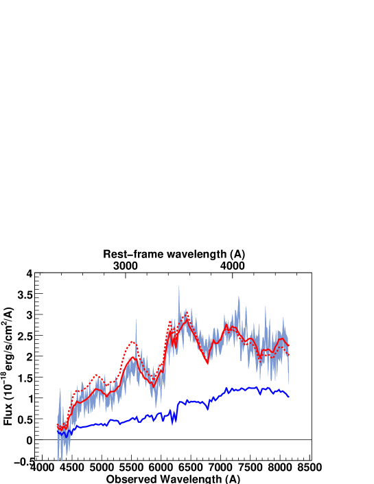
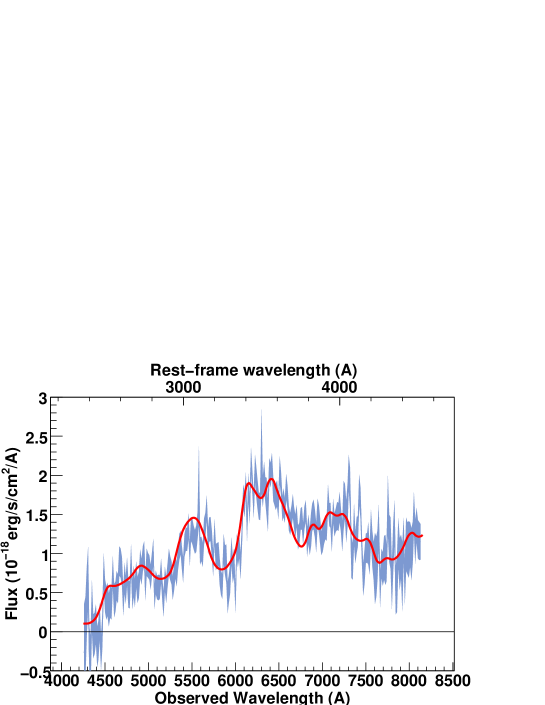
Figure 107: SNLS- 05D2dt807: a SN Ia supernova at z=0.574. The spectrum phase is -1.7. A E(3) host model has been subtracted.

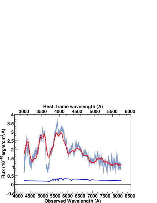
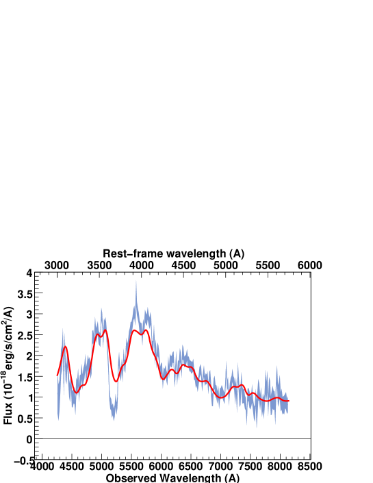
Figure 108: SNLS- 05D2dw807: a SN Ia supernova at z=0.417. The spectrum phase is -5.3. A S0(1) host model has been subtracted. Note that the model is unable to reproduce the deep Ca ii feature at rest-frame 3700 $\AA$.

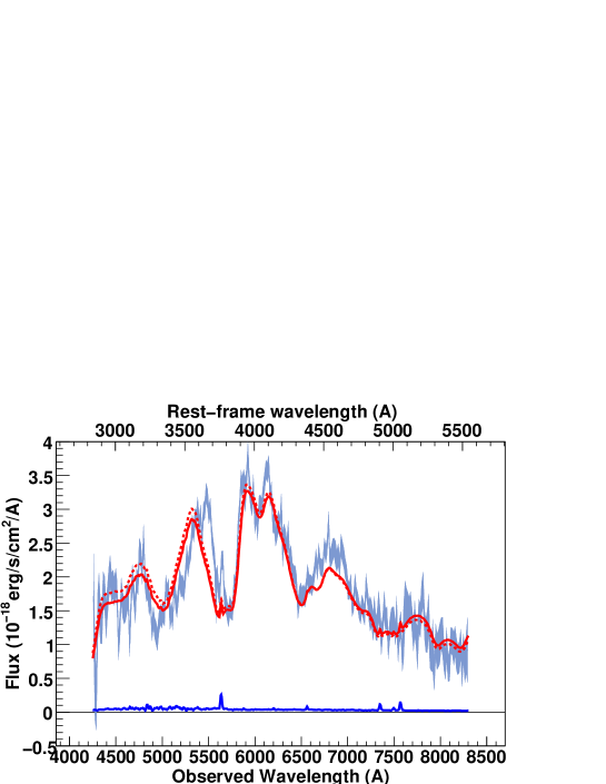
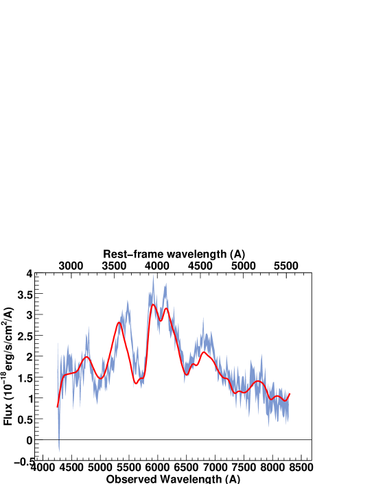
Figure 109: SNLS- 05D2dy805: a SN Ia supernova at z=0.51. The spectrum phase is 1.1. A Sb-Sc host model has been subtracted. Note that the Ca ii feature at rest-frame 3700 $\AA$ is narrower than in the model.

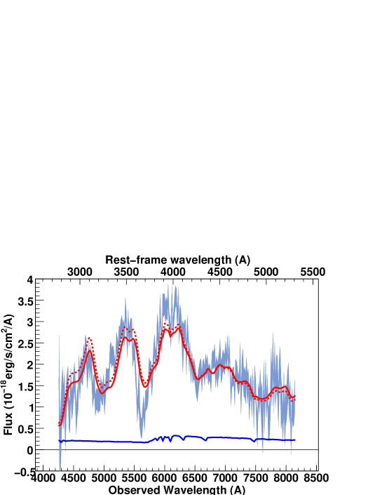
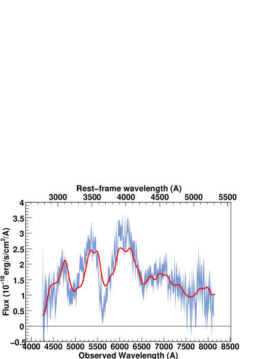
Figure 110: SNLS- 05D2eb805: a SN Ia supernova at z=0.534. The spectrum phase is -4.7. A S0(1) host model has been subtracted. Note that the model is unable to reproduce the deep Ca ii feature at rest-frame 3700 $\AA$.

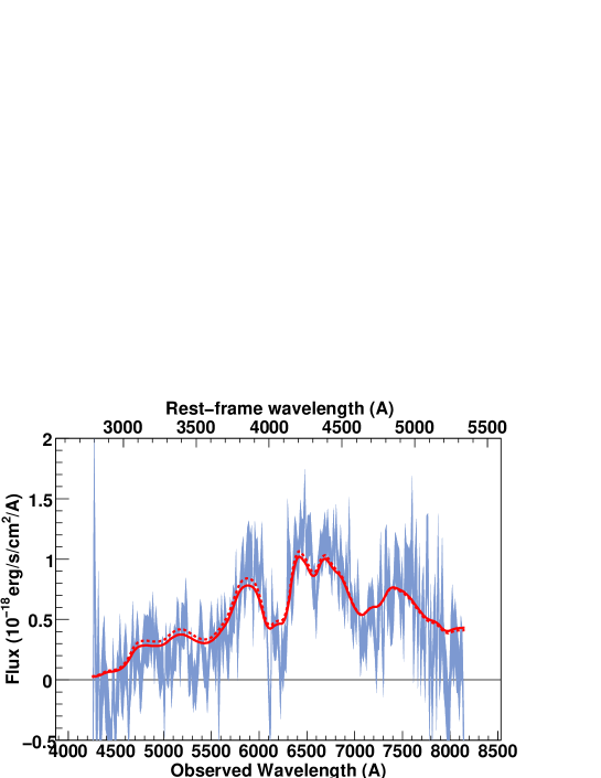
Figure 111: SNLS- 05D2ec805: a SN Ia supernova at z=0.640. The spectrum phase is 2.7. Best-fit obtained for a model with no host galaxy component.

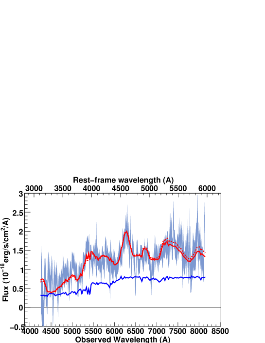
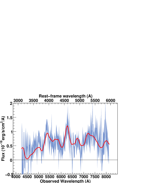
Figure 112: SNLS- 05D2ei833: a SN Ia$\star$ supernova at z=0.366. The spectrum phase is 16.9. A S0(4) host model has been subtracted.

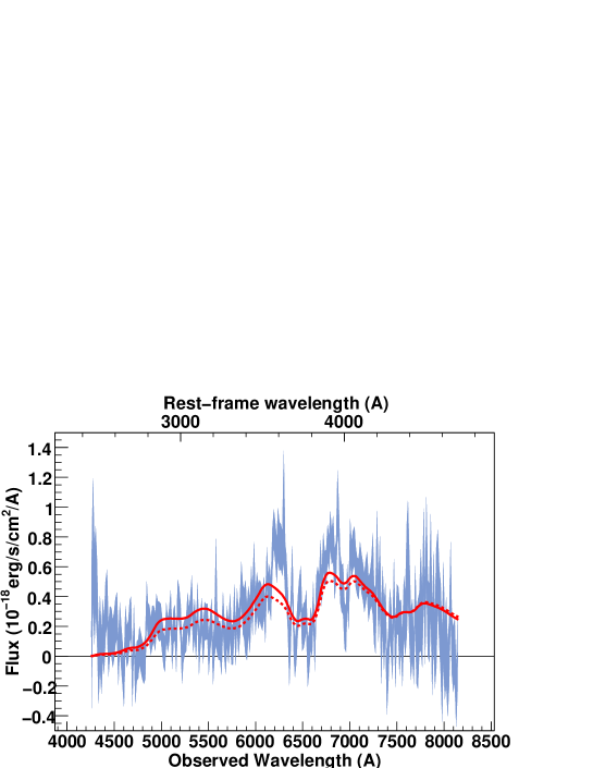
Figure 113: SNLS- 05D2fq827: a SN Ia supernova at z=0.733. The spectrum phase is 2.1. Best-fit obtained for a model with no host galaxy component.

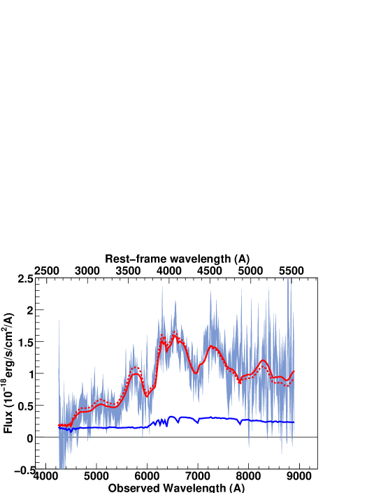
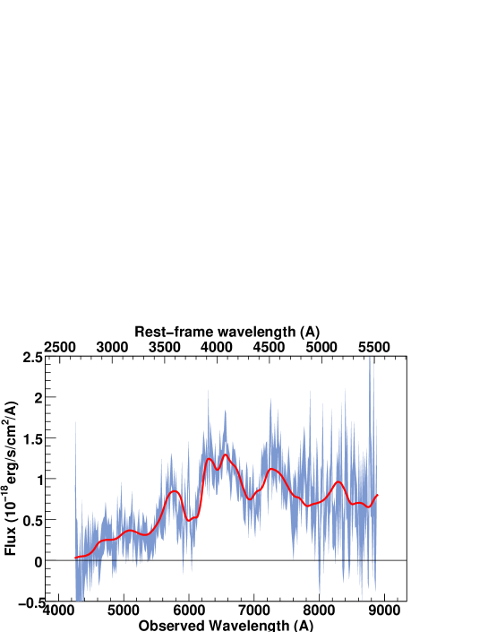
Figure 114: SNLS- 05D2he833: a SN Ia supernova at z=0.608. The spectrum phase is 3.0. A E(1) host model has been subtracted.

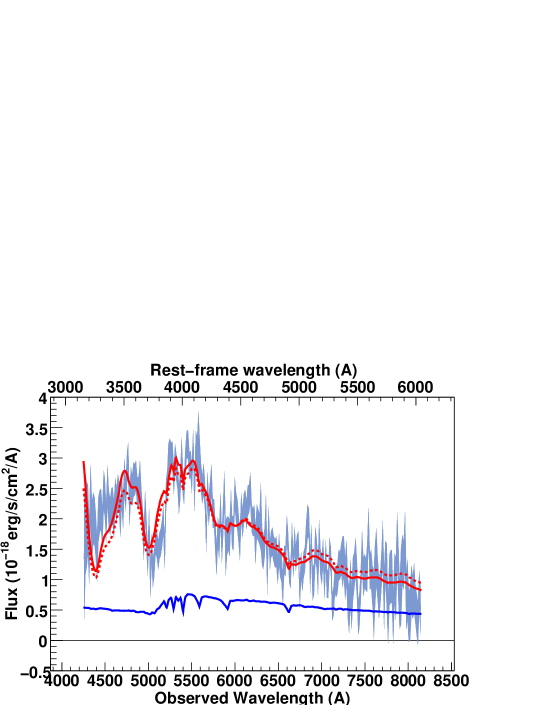
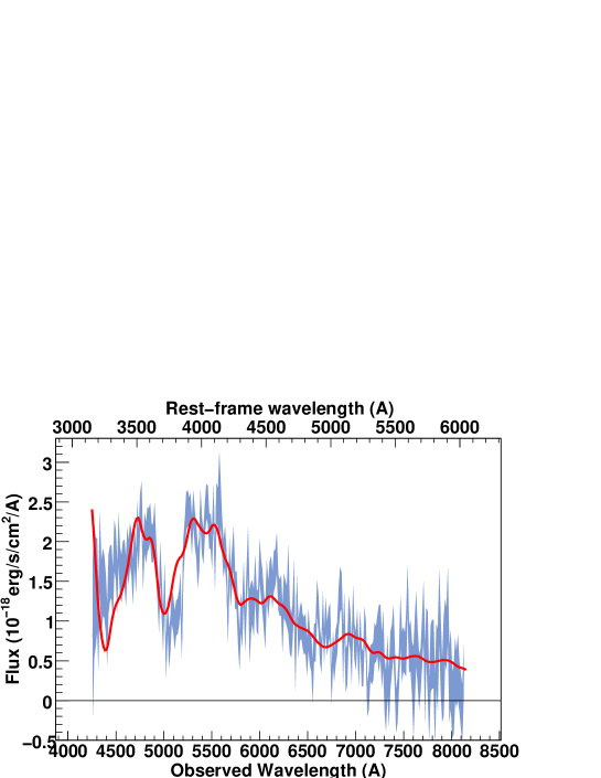
Figure 115: SNLS- 05D2ie829: a SN Ia supernova at z=0.348. The spectrum phase is -8.9. A Sc(4) host model has been subtracted.

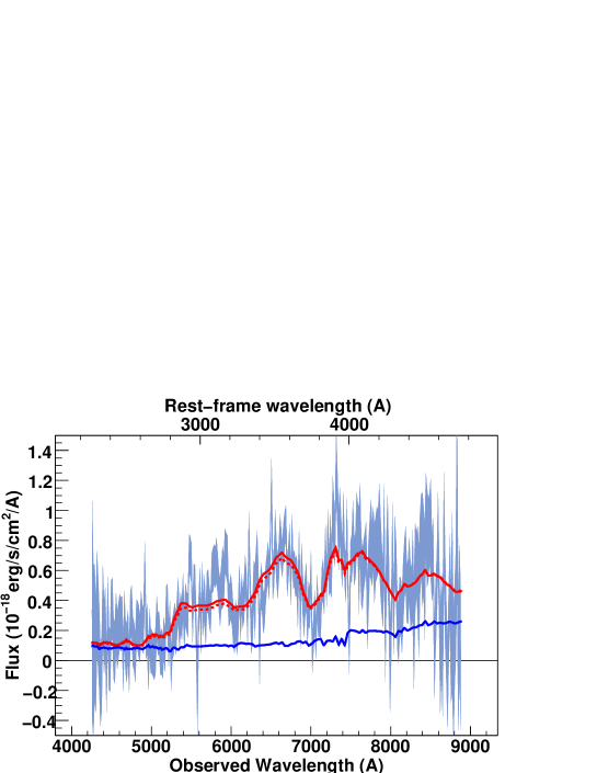
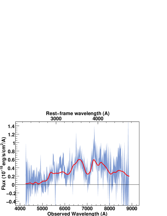
Figure 116: SNLS- 05D2nn1071: a SN Ia supernova at z=0.87. The spectrum phase is -1.3. A Sa(8) host model has been subtracted.

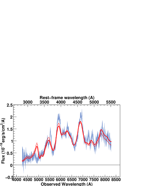
Figure 117: SNLS- 05D4af914: a SN Ia supernova at z=0.499. The spectrum phase is 11.3. Best-fit obtained for a model with no host galaxy component.

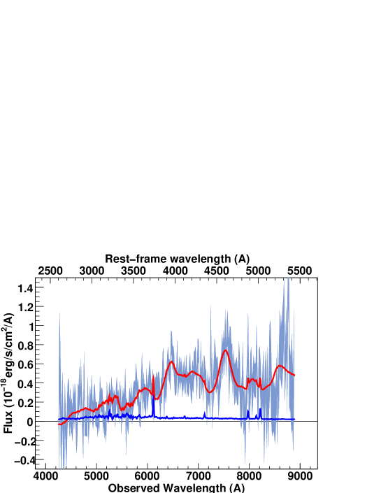
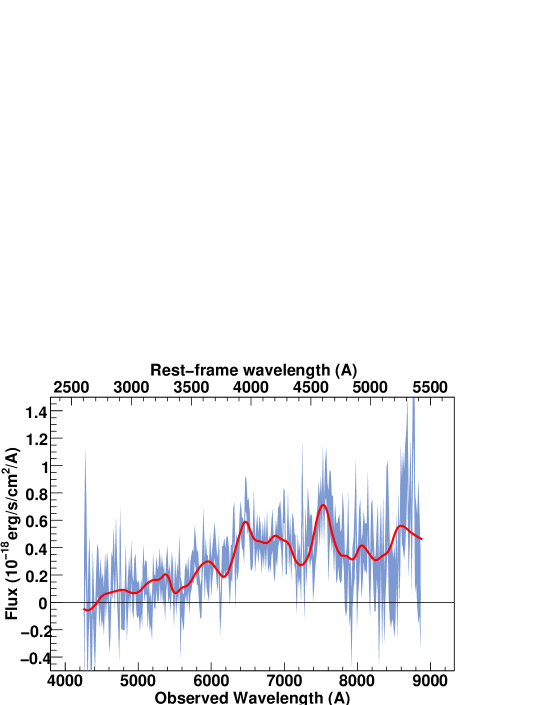
Figure 118: SNLS- 05D4ag922: a SN Ia$\star$ supernova at z=0.64. The spectrum phase is 14.0. A Sb-Sc host model has been subtracted.

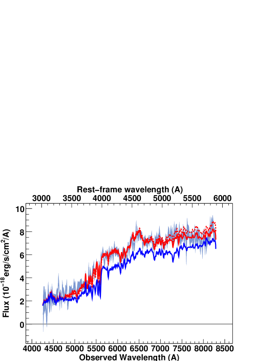
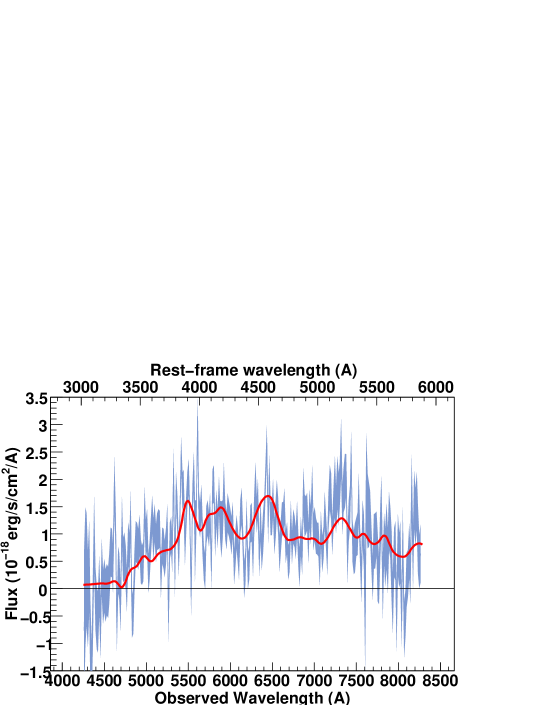
Figure 119: SNLS- 05D4ay914: a SN Ia$\star$ supernova at z=0.408. The spectrum phase is 8.2. A Sa-Sb host model has been subtracted.

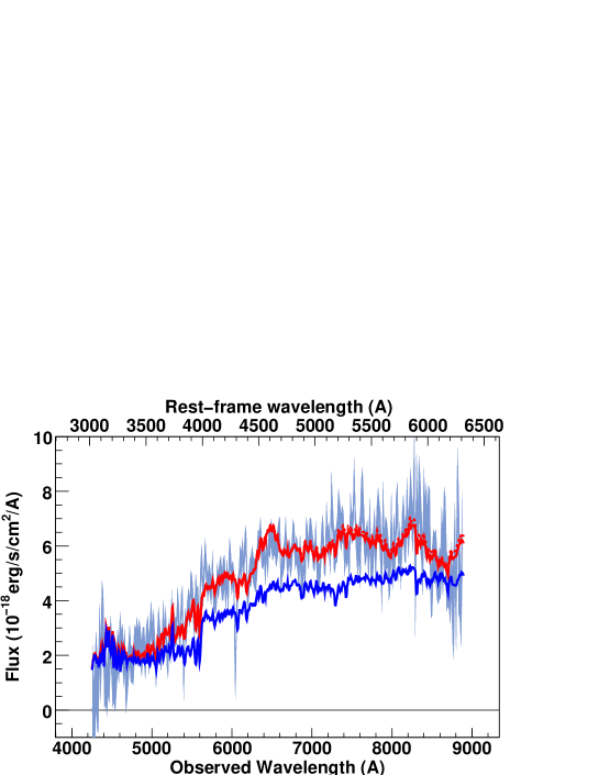
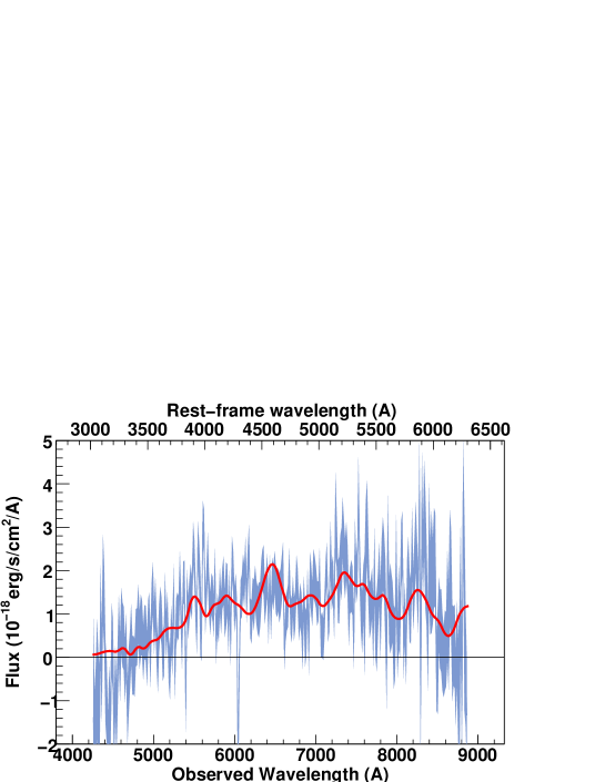
Figure 120: SNLS- 05D4ay916: a SN Ia$\star$ supernova at z=0.408. The spectrum phase is 9.6. A Sa-Sb host model has been subtracted.

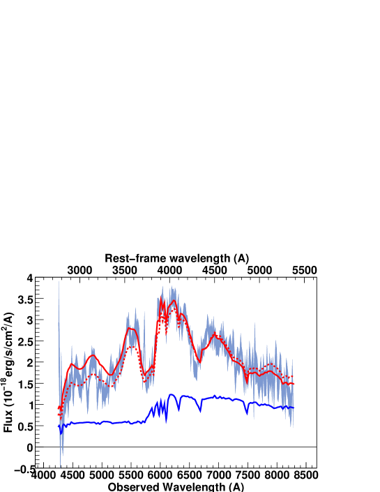
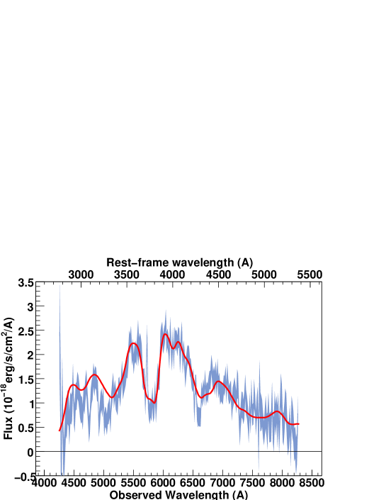
Figure 121: SNLS- 05D4be918: a SN Ia supernova at z=0.537. The spectrum phase is 3.9. A E(1) host model has been subtracted.

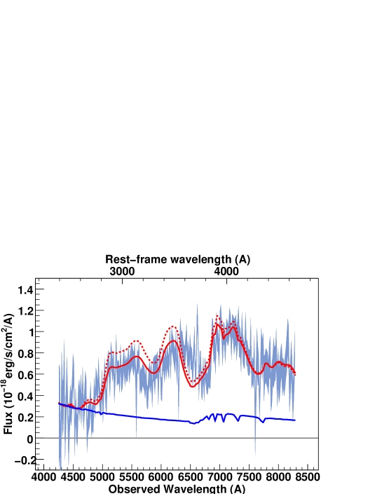
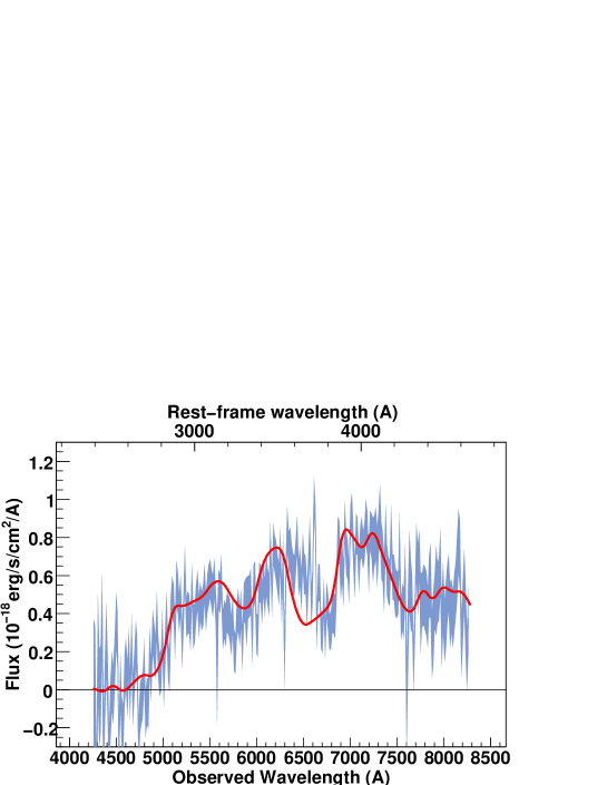
Figure 122: SNLS- 05D4bi918: a SN Ia supernova at z=0.775. The spectrum phase is -1.5. A Sc(1) host model has been subtracted.

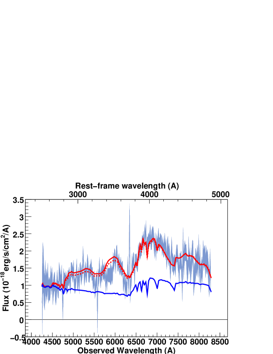
Figure 123: SNLS- 05D4bj921: a SN Ia supernova at z=0.701. The spectrum phase is -2.0. A Sc(9) host model has been subtracted.

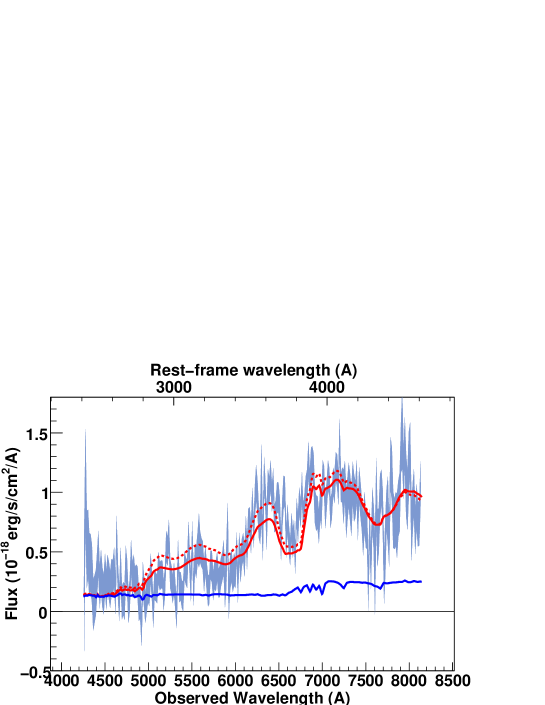
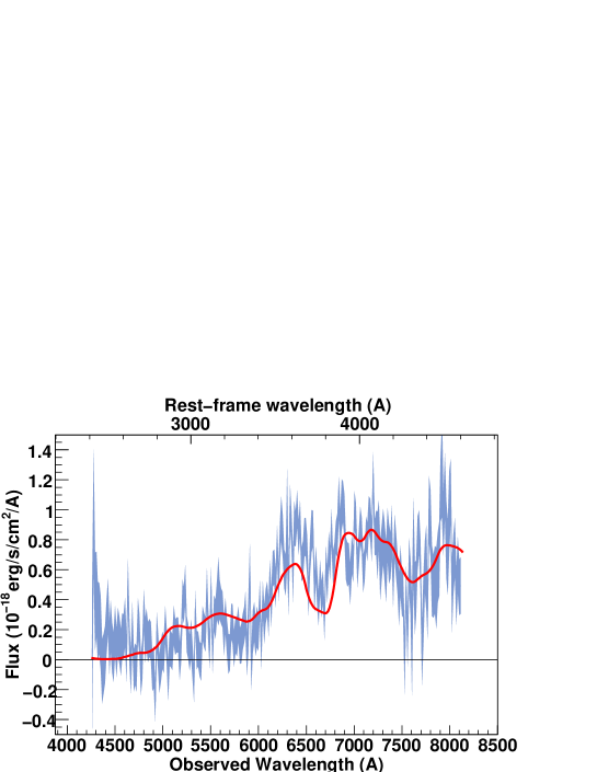
Figure 124: SNLS- 05D4cn952: a SN Ia supernova at z=0.763. The spectrum phase is 4.7. A S0(1) host model has been subtracted.

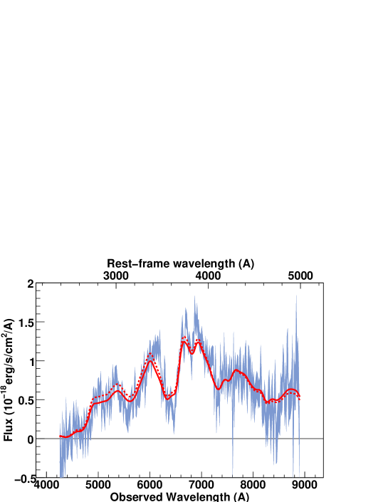
Figure 125: SNLS- 05D4cq946: a SN Ia supernova at z=0.701. The spectrum phase is -0.1. Best-fit obtained for a model with no host galaxy component.

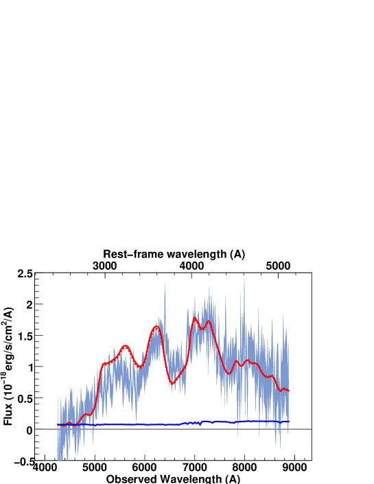
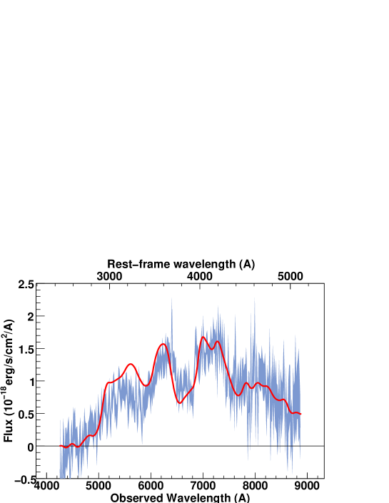
Figure 126: SNLS- 05D4cs946: a SN Ia supernova at z=0.79. The spectrum phase is -1.7. A Sc(12) host model has been subtracted.

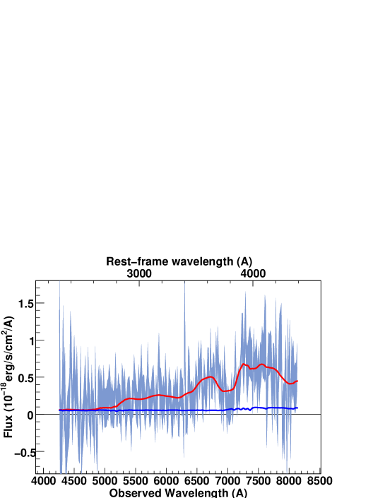
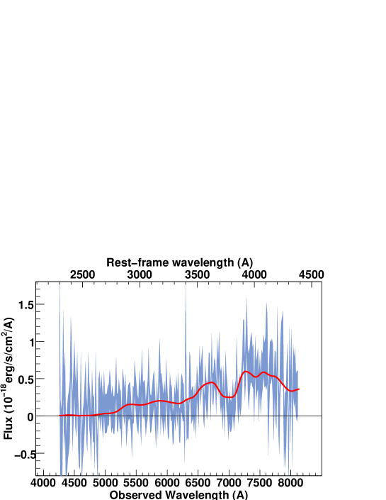
Figure 128: SNLS- 05D4dw983: a SN Ia supernova at z=0.855. The spectrum phase is 4.7. A Sc(12) host model has been subtracted.

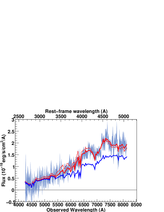
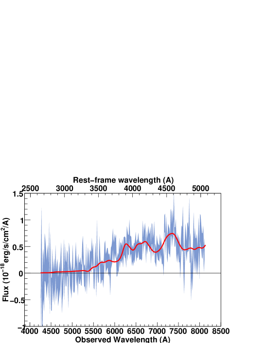
Figure 129: SNLS- 05D4ef997: a SN Ia$\star$ supernova at z=0.605. The spectrum phase is 3.5. A E(3) host model has been subtracted.

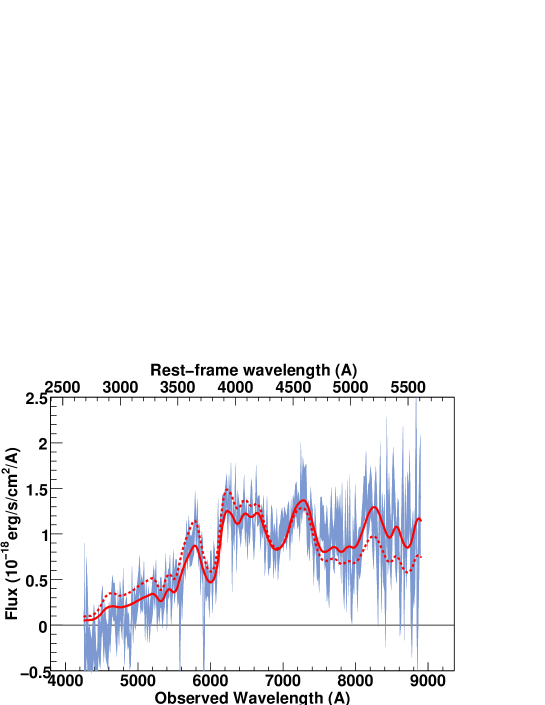
Figure 130: SNLS- 05D4ej1000: a SN Ia supernova at z=0.585. The spectrum phase is 7.6. Best-fit obtained for a model with no host galaxy component.

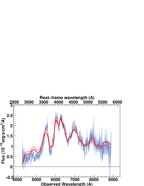
Figure 131: SNLS- 05D4ek999: a SN Ia supernova at z=0.536. The spectrum phase is 2.1. Best-fit obtained for a model with no host galaxy component.

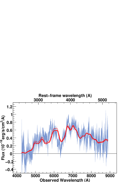
Figure 132: SNLS- 05D4ev985: a SN Ia supernova at z=0.722. The spectrum phase is -3.6. Best-fit obtained for a model with no host galaxy component.

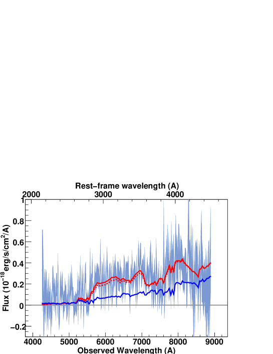
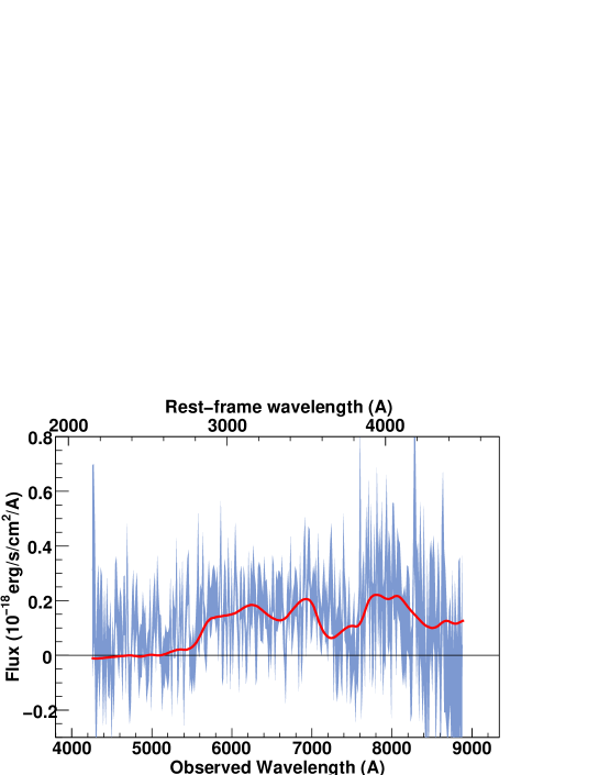
Figure 133: SNLS- 05D4fe1000: a SN Ia$\star$ supernova at z=0.984. The spectrum phase is -2.0. A E(3) host model has been subtracted.

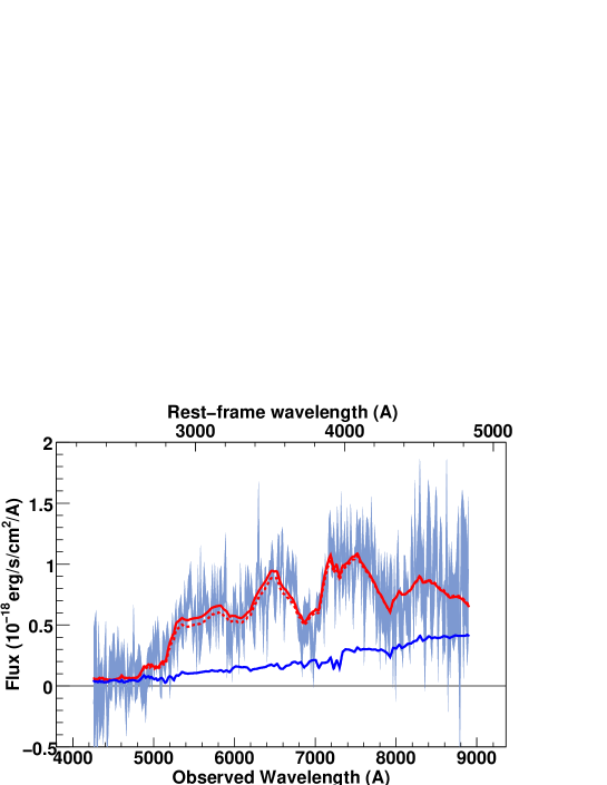
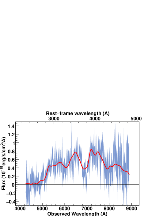
Figure 135: SNLS- 05D4fg1002: a SN Ia supernova at z=0.839. The spectrum phase is -0.3. A S0(5) host model has been subtracted.

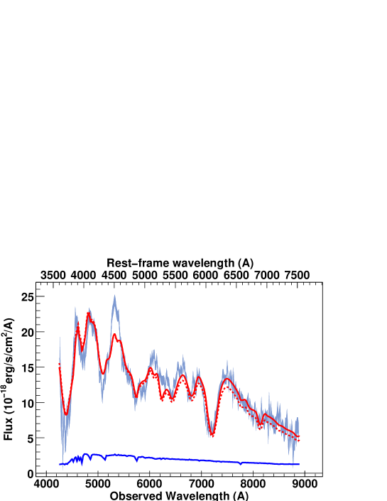
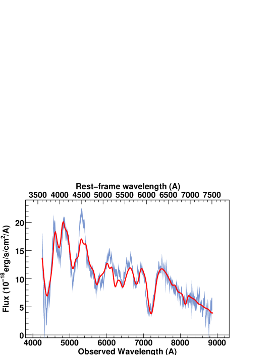
Figure 136: SNLS- 06D1ab1100: a SN Ia supernova at z=0.182. The spectrum phase is -4.4. A E(7) host model has been subtracted. Note that the model is unable to reproduce the large feature at rest-frame 4500 $\AA$.

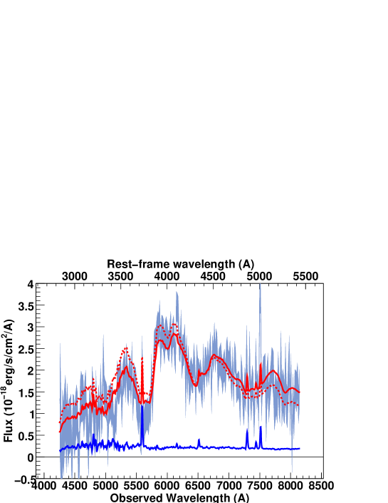
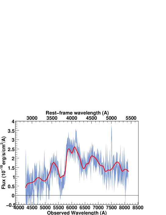
Figure 137: SNLS- 06D2bk1135: a SN Ia supernova at z=0.499. The spectrum phase is 0.9. A Sb-Sc host model has been subtracted.

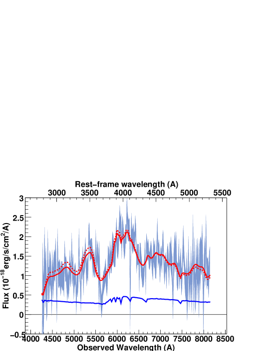
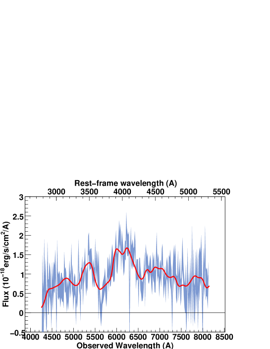
Figure 138: SNLS- 06D2ca1153: a SN Ia supernova at z=0.531. The spectrum phase is 0.0. A Sd(5) host model has been subtracted.

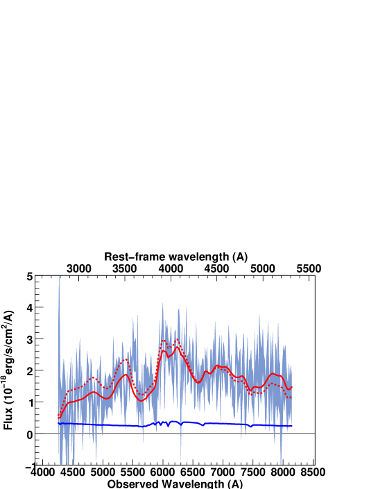
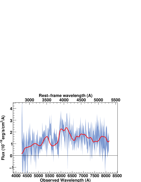
Figure 139: SNLS- 06D2ca1154: a SN Ia supernova at z=0.531. The spectrum phase is 0.7. A Sd(3) host model has been subtracted.

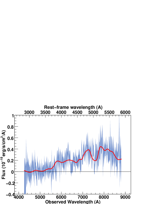
Figure 140: SNLS- 06D2cb1155: a SN Ia$\star$ supernova at z=1.00. The spectrum phase is 3.0. Best-fit obtained for a model with no host galaxy component.

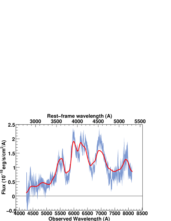
Figure 141: SNLS- 06D2cc1153: a SN Ia supernova at z=0.532. The spectrum phase is 3.3. Best-fit obtained for a model with no host galaxy component.

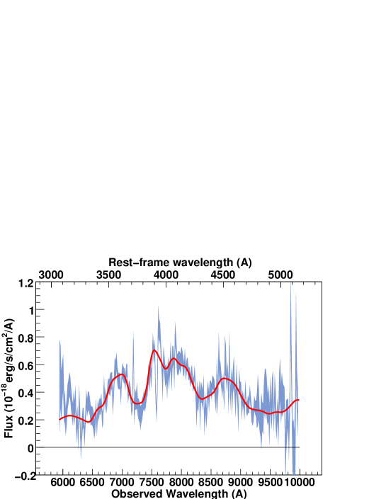
Figure 142: SNLS- 06D2cd1157: a SN Ia supernova at z=0.930. Spectrum obtained with the 300I Grism on FORS2. The spectrum phase is 4.2. Best-fit obtained for a model with no host galaxy component.

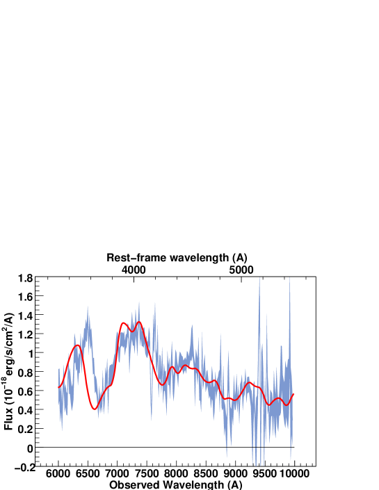
Figure 143: SNLS- 06D2ce1156: a SN Ia supernova at z=0.82. Spectrum obtained with the 300I Grism on FORS2. The spectrum phase is 0.0. Best-fit obtained for a model with no host galaxy component.

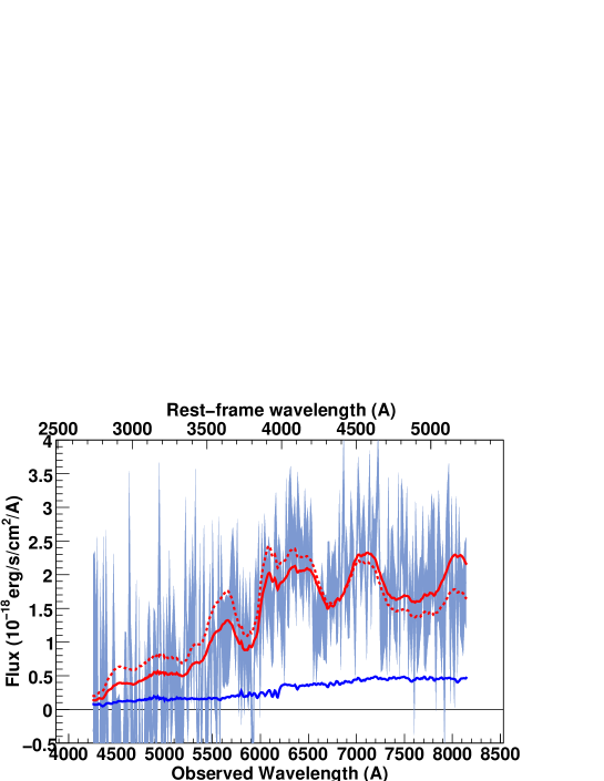
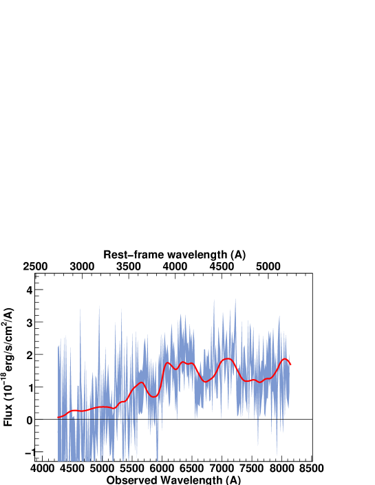
Figure 144: SNLS- 06D2ck1162: a SN Ia$\star$ supernova at z=0.552. The spectrum phase is 7.7. A Sa-Sb host model has been subtracted.

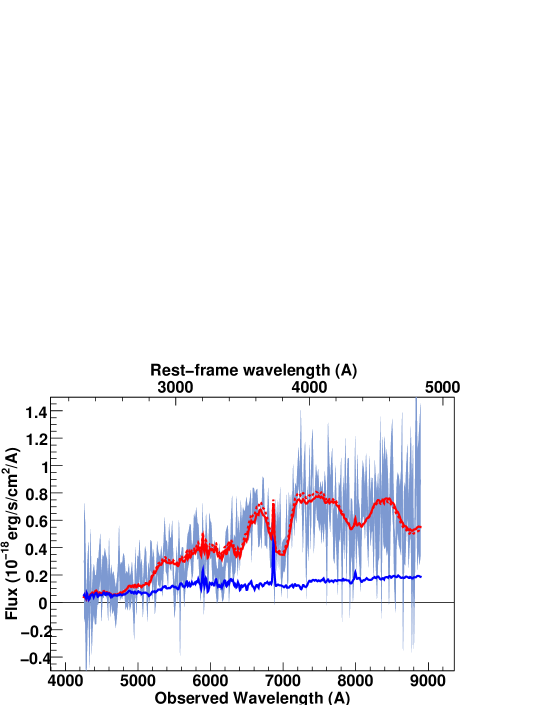
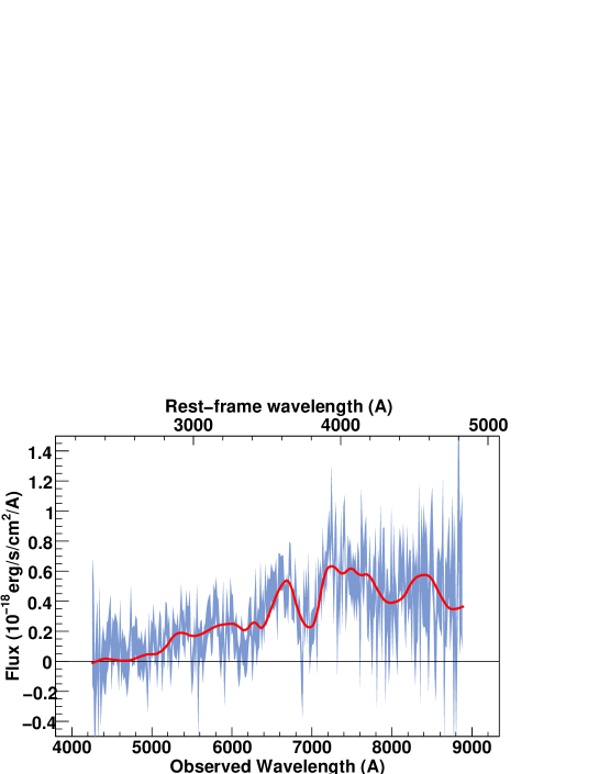
Figure 145: SNLS- 06D2ga1241: a SN Ia$\star$ supernova at z=0.84. The spectrum phase is 5.4. A Sb-Sc host model has been subtracted.

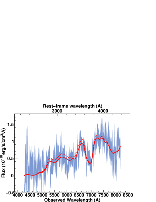
Figure 146: SNLS- 06D4ce1295: a SN Ia supernova at z=0.85. The spectrum phase is 2.7. Best-fit obtained for a model with no host galaxy component.

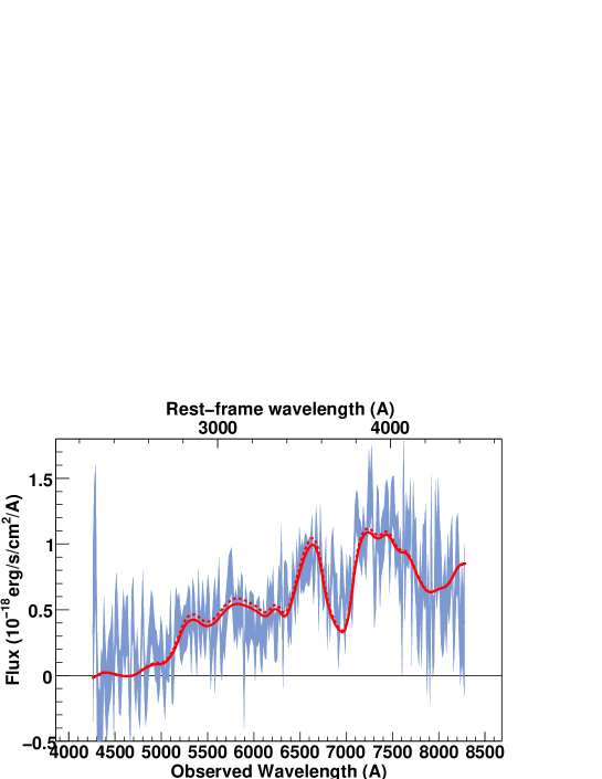
Figure 147: SNLS- 06D4ce1296: a SN Ia supernova at z=0.85. The spectrum phase is 3.3. Best-fit obtained for a model with no host galaxy component.

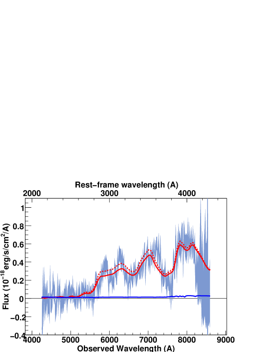
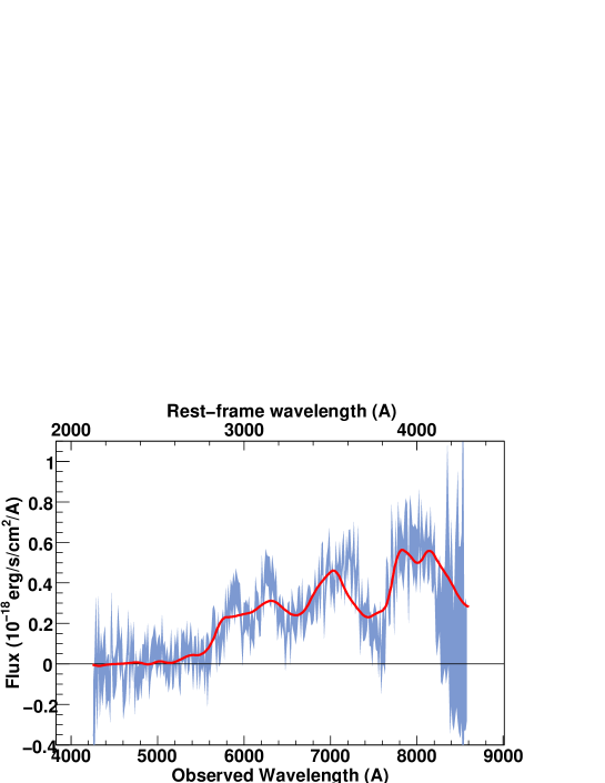
Figure 148: SNLS- 06D4cl1297: a SN Ia supernova at z=1.00. The spectrum phase is -2.5. A E(1) host model has been subtracted.

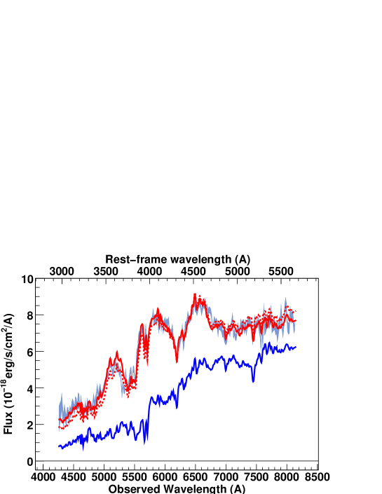
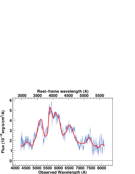
Figure 149: SNLS- 06D4co1306: a SN Ia supernova at z=0.437. The spectrum phase is 3.5. A E-S0 host model has been subtracted.

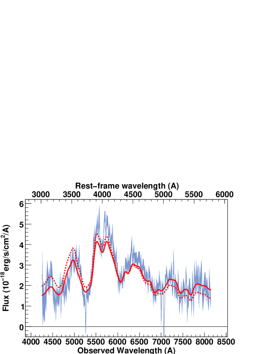
Figure 150: SNLS- 06D4cq1306: a SN Ia supernova at z=0.411. The spectrum phase is -1.4. Best-fit obtained for a model with no host galaxy component.

References

Astier et al. (2006)
Astier, P., Guy, J., Regnault, N., et al. 2006, A&A, 447, 31
Balland et al. (2007)
Balland, C., Mouchet, M., Amanullah, R., et al. 2007, A&A, 464, 827
Balland et al. (2006)
Balland, C., Mouchet, M., Pain, R., et al. 2006, A&A, 445, 387
Basa et al. (2009)
Basa, S., et al. 2009, A&A, in prep.
Baumont (2007)
Baumont, S. 2007, PhD thesis, Univ. D. Diderot, Paris 7,
supernovae.in2p3.fr/ baumont/outreach/baumont_these.pdf
Baumont et al. (2008)
Baumont, S., Balland, C., Astier, P., et al. 2008, A&A, 491, 567
Bazin et al. (2009)
Bazin, G., Palanque-Delabrouille, N., Rich, J., et al. 2009, A&A, 499,
653
Blondin et al. (2006)
Blondin, S., Dessart, L., Leibundgut, B., et al. 2006, AJ, 131, 1648
Blondin & Tonry (2007)
Blondin, S. & Tonry, J. L. 2007, ApJ, 666, 1024
Blondin et al. (2005)
Blondin, S., Walsh, J. R., Leibundgut, B., & Sainton, G. 2005, A&A,
431, 757
Boulade et al. (2003)
Boulade, O., Charlot, X., Abbon, P., et al. 2003, in Presented at the
Society of Photo-Optical Instrumentation Engineers (SPIE) Conference, Vol.
4841, Instrument Design and Performance for Optical/Infrared Ground-based
Telescopes. Edited by Iy e, Masanori; Moorwood, Alan F. M. Proceedings of the
SPIE, Volume 4841, pp. 72-81 (2003)., ed. M. Iye & A. F. M. Moorwood,
72–81