Molecular wires acting as quantum heat ratchets

Abstract

We explore heat transfer in molecular junctions between two leads in the absence of a finite net thermal bias. The application of an unbiased, time-periodic temperature modulation of the leads entails a dynamical breaking of reflection symmetry, such that a directed heat current may emerge (ratchet effect). In particular, we consider two cases of adiabatically slow driving, namely (i) periodic temperature modulation of only one lead and (ii) temperature modulation of both leads with an ac driving that contains a second harmonic, thus generating harmonic mixing. Both scenarios yield sizeable directed heat currents which should be detectable with present techniques. Adding a static thermal bias, allows one to compute the heat current-thermal load characteristics which includes the ratchet effect of negative thermal bias with positive-valued heat flow against the thermal bias, up to the thermal stop-load. The ratchet heat flow in turn generates also an electric current. An applied electric stop-voltage, yielding effective zero electric current flow, then mimics a solely heat-ratchet-induced thermopower (“ratchet Seebeck effect”), although no net thermal bias is acting. Moreover, we find that the relative phase between the two harmonics in scenario (ii) enables steering the net heat current into a direction of choice.

I Introduction

In recent years, we have witnessed the development of nano-devices based on molecular wires Nitzan1 ; Reed1 ; hanggiCP ; kohler_pr ; TaoNJ1 . One of their essential features is that the electric current through them can be controlled effectively. One approach to such transport control is based on conformational changes of the molecule Reed2 ; Kuekes1 ; ZhangC1 . Another scheme relies on the dipole interaction between the molecular wire and a tailored laser field Lehmann1 ; Lehmann2 ; LiGQ1 ; Franco1 ; Kohler1 . A further approach employs gate voltages acting on the wire YangZQ1 ; Ghosh1 ; JiangF1 . The latter allows a transistor-like control which has already been demonstrated experimentally XiaoK1 ; SunY1 ; XuB1 . It is therefore interesting to explore as well the related control of heat transport.

In general, heat transport through a molecular junction involves the combined effect of electron as well as phonon transfer processes. Control of phonon transport is much more complicated since the phonon number is not conserved. Nevertheless, the field of phononics, i.e. control and manipulation of phonons in nanomaterials, has emerged WangL1 . This includes functional devices, such as thermal diodes TD1 ; TD2 ; TD3 ; TD4 ; TD5 ; TD6 ; TD7 , thermal transistors TT1 ; TT2 , thermal logic gates TLG , and thermal memories TM based on the presence of a static temperature bias. The corresponding theoretical research has been accompanied by experimental efforts on nanosystems. In particular, solid-state thermal diodes have been realized with asymmetric nanotubes Ex_TD1 and with semiconductor quantum dots Ex_TD2 .

Upon harvesting ideas from the field of Brownian motors BM1 ; BM2 ; BM3 ; BM4 ; BM5 — originally devised for particle transport — a classical Brownian heat engine has been proposed to rectify and steer heat current in nonlinear lattice structures BHM1 ; BHM2 . In the absence of any static non-equilibrium bias, a non-vanishing net heat flow can be induced by unbiased, temporally alternating bath temperatures combined with nonlinear interactions among neighboring lattice sites. This so obtained directed heat current can be readily controlled to reverse direction. If, in addition, a thermal bias across the molecule is applied, a heat current can then typically be directed even against an external thermal bias. This setup is therefore rather distinct from adiabatic and nonadiabatic electron heat pumps which involve photon assisted transmission and reflection processes in presence of irradiating photon sources kohler_pr ; rey ; arrachea .

In this work, we investigate the possibility of steering heat through a molecular junction in the presence of a gating mechanism. In doing so, the bath temperatures of adjacent leads are subjected to slow, time-periodic modulations. Both the electronic and the phononic heat current are considered, as is sketched in Fig. 1. A finite directed ratchet heat current requires breaking reflection symmetry. This can be achieved by spatial asymmetries in combination with non-equilibrium fields BM1 ; BM2 ; BM3 ; BM4 ; BM5 or in a purely dynamical way SB1 ; SB2 ; SB3 ; SB4 ; SB5 . In this work we focus on an unbiased temporal temperature variation in the connecting leads.

Figure 1: Setup of a molecular junction whose electronic level $E_{1}$ can be gated, while the vibrational frequency $\omega_{1}$ is fixed. The lead temperatures $T_{\text{L}(\text{R})}(t)$ are subjected to time-periodic modulations.

This paper is organized as follows: In Section II, we specify the physical assumptions and introduce our model together with the basic theoretical concepts for directing heat current across a short, gated molecular junction formed by a harmonically oscillating molecule. The heat flux is induced by temperature modulations in the contacting leads. Section III presents the results for case (i) where the temperature is modulated in one lead only. We elaborate on the phenomenon of pumping heat against a static thermal bias and consider the resulting thermoelectric power. In Section IV, we consider case (ii) with both lead temperatures periodically, but asymmetrically modulated. A finite directed heat current emerges from harmonic mixing of different frequencies, which entails dynamical symmetry breaking. Since the leading order of this heat current is of third order only in the driving strengths, the overall rectification is weaker as compared to case (i) where the heat flux starts out at second order in the driving amplitude. The latter scheme with its symmetric static parameters, however, provides a more efficient control scenario: The direction of the resulting heat current can be readily reversed either by a gate voltage or by adjusting the relative phase shift within the harmonic mixing signal for the temperature modulation. Section V contains a summary and an outlook.

II Physical assumptions, model, and ballistic heat transfer

We consider a molecular junction between two leads and a static gate voltage acting on the junction. Heat transport from both electrons and phonons is taken into account. Since we focus on coherent transport in a short molecular wire Nitzan ; segalnitzan2005 ; segal2006 , electron-phonon interaction can be ignored. Moreover, we treat ballistic heat transfer for the electron system and the phonon system in the absence of anharmonic interactions and dissipative intra-wire scattering processes. Then, the heat flux can be obtained in terms of a Landauer-type expression involving corresponding temperature-independent transmission probabilities for both the electrons sivan ; zheng and the phonons ciraci ; segal . The total Hamiltonian can thus be separated into electron and phonon part, i.e.,

$$H=H^{\text{el}}+H^{\text{ph}},$$ (1)

each of which consisting of a wire contribution, a lead contribution, and an interaction term, such that

$$H^{\text{el}(\text{ph})}=H^{\text{el}(\text{ph})}_{\text{wire}}+H^{\text{el}(\text{ph})}_{\text{leads}}+H^{\text{el}(\text{ph})}_{\text{contacts}}\,.$$ (2)

The short molecular wire is modeled as a single energy level and one harmonic phonon mode only. Then the Hamiltonian of the wire electron in tight-binding approximation reads

$$H^{\text{el}}_{\text{wire}}=E_{1}\left.|1\right>\left<1|\right.\,,$$ (3)

where $E_{1}$ describes the on-site energy of the tight-binding level which can be shifted via a gate voltage. The electrons in the leads are modeled as ideal electron gases, i.e.,

$$H^{\text{el}}_{\text{leads}}=H_{\text{L}}+H_{\text{R}}=\sum_{q}\epsilon_{\text{L}q}c^{\dagger}_{\text{L}q}c_{\text{L}q}+\sum_{q}\epsilon_{\text{R}q}c^{\dagger}_{\text{R}q}c_{\text{R}q}\,,$$ (4)

where $c^{\dagger}_{lq}$ creates an electron in state $\left.|lq\right>$ of lead $l=\mathrm{\text{L},\text{R}}$. The electron tunneling Hamiltonian

$$H^{\text{el}}_{\text{contacts}}=\sum_{q}(V_{\text{L}q}c^{\dagger}_{\text{L}q}c_{1}+V_{\text{R}q}c^{\dagger}_{\text{R}q}c_{1})+\text{h.c.}\,,$$ (5)

establishes the contact between the wire and the leads. This tunneling coupling is characterized by the spectral density $\Gamma_{l}(\epsilon)=2\pi\sum_{q}|V_{lq}|^{2}\delta(\epsilon-\epsilon_{lq})$. We assume symmetric coupling within a wide-band limit such that $\Gamma_{l}(\epsilon)=\Gamma$.

The phonon mode is represented by a harmonic oscillator with the Hamiltonian

$$H^{\text{ph}}_{\text{wire}}=\frac{P^{2}}{2M}+\frac{1}{2}M\omega^{2}_{1}Q^{2}\,,$$ (6)

where $Q$ and $P$ denote the position and the momentum operator, respectively, $M$ denotes the atom mass and $\omega_{1}$ the characteristic phonon frequency of wire. The phonon bath and its bilinear coupling to the wire system is described by

$$\begin{split}H^{\text{ph}}_{\text{leads}}&+H^{\text{ph}}_{\text{contacts}}\\ &=\sum_{l,k}\left\{\frac{p^{2}_{lk}}{2m_{l}}+\frac{m_{l}\omega^{2}_{lk}}{2}\left(x_{lk}-\frac{g_{l}Q}{m_{l}\omega_{lk}}\right)^{2}\right\},\end{split}$$ (7)

where $x_{lk},p_{lk},\omega_{lk}$ are the position operators, momentum operators, and frequencies associated with the bath degrees of freedom; $m_{l}$ are the masses and $g_{l}=g_{\text{L}}=g_{\text{R}}=g$ represent a symmetric phonon wire-lead coupling strength for lead $l=\text{L},\text{R}$. The position and momentum operators can be expressed in terms of the creation and annihilation operators for phonons as $x_{lk}=\sqrt{\hbar/2m_{l}\omega_{lk}}(a^{\dagger}_{lk}+a_{lk})$ and $p_{lk}=i\sqrt{\hbar m_{l}\omega_{lk}/2}(a^{\dagger}_{lk}-a_{lk})$.

Throughout the following we assume that slow, time modulated temperature system acting on the baths are always sufficiently slow so that a thermal quasi-equilibrium for the molecular wire system can assumed. The heat transport then obeys the adiabatic, exact coherent quantum transport laws as discussed in the next subsection, see Eq. (13) and (14) below.

II.1 Adiabatic modulation of the lead temperatures

At thermal equilibrium with temperature $T=T_{\mathrm{\text{L}}}=T_{\mathrm{\text{R}}}$ with equal electro-chemical potentials $\mu_{\mathrm{\text{L}}}=\mu_{\mathrm{\text{R}}}=\mu$, the density matrix for the leads read $\rho_{l}\propto e^{-(H^{\text{ph}}_{l}+H^{\text{el}}_{l}-\mu_{l}N_{l})/k_{\text{B}}T_{l}}$, where $N_{l}=\sum_{q}c^{\dagger}_{lq}c_{lq}$ is the number of electrons in lead $l=\text{L},\text{R}$ and $k_{\text{B}}T_{l}$ denotes the present lead temperature multipled by the the Boltzmann constant. To induce shuttling of heat, we invoke a non-equilibrium situation via an adiabatically slow temperature modulation $T_{l}(t)$ in the leads. The latter can be realized experimentally, for example, by use of a heating/cooling circulator laser . Then the expectation values of the electron and phonon lead operators then read

$$\langle c^{\dagger}_{l^{\prime}q^{\prime}}c_{lq}\rangle =f_{l}(\epsilon_{q},T_{l}(t))\delta_{ll^{\prime}}\delta_{qq^{\prime}}\,,$$ (8)

$$\langle a^{\dagger}_{l^{\prime}k^{\prime}}a_{lk}\rangle =n_{l}(\omega_{k},T_{l}(t))\delta_{ll^{\prime}}\delta_{kk^{\prime}},$$ (9)

where $f_{l}(\epsilon,T_{l}(t))=[\text{exp}((\epsilon-\mu_{l})/k_{\text{B}}T_{l}(t))+1]^{-1}$ and $n_{l}(\omega,T_{l}(t))=[\text{exp}(\hbar\omega/k_{\text{B}}T_{l}(t))-1]^{-1}$ denote the Fermi-Dirac distribution and the Bose-Einstein distribution, respectively, which both inherit a time-dependence from the temperature modulation. This implies a time-scale separation which is justified by the fact that laser heating of a metallic system, the electrons undergo rather fast thermalization fast1 ; fast2 ; fast3 ; fast4 . The corresponding relaxation times stem from electron-electron and electron-phonon interaction, and for a typical metal is in the order of a few fs or ps, respectively ts1 ; ts2 . Therefore, the changes of the lead temperatures occur on a time-scale much smaller than the thermal fluctuations itself, i.e. $2\pi/\Omega\gg 1$ ps.

The time-varying lead temperatures $T_{\text{L}}(t)$ and $T_{\text{R}}(t)$ are assumed to be time-periodic $T_{\text{L}(\text{R})}(t)=T_{\text{L}(\text{R})}(t+2\pi/\Omega)$, where $T_{0}=\overline{T_{\text{L}}(t)}=\overline{T_{\text{R}}(t)}$ denotes the time-averaged environmental reference temperature. This implies a vanishing temperature bias

$$\overline{\Delta T(t)}\equiv\overline{T_{\text{L}}(t)-T_{\text{R}}(t)}=0\;.$$ (10)

In the long-time limit, the time-dependent, asymptotic heat current $J_{Q}(t)=J^{\text{el}}_{Q}(t)+J^{\text{ph}}_{Q}(t)$ assumes the periodicity $2\pi/\Omega$ of the external driving field

$$J_{Q}(t)=J_{Q}(t+{2\pi}/{\Omega}).$$ (11)

Henceforth we focus on the stationary heat current $\overline{J_{Q}}$ which follows from the average over a full driving period:

$$\overline{J_{Q}}=\frac{\Omega}{2\pi}\int_{0}^{2\pi/\Omega}J_{Q}(t)dt.$$ (12)

If the lead temperatures are modulated slowly enough (adiabatic temperature rocking), the dynamical thermal bias $\Delta T(t)$ can be viewed as a static bias at time $t$ in the adiabatic limit $\Omega\rightarrow 0$. Thus the asymptotic electron and phonon heat currents $J^{\text{el}(\text{ph})}_{Q}(t)$ can be expressed by the Landauer-type formula for electron heat flux sivan ; zheng and for the phonon heat flux rego ; ciraci ; segal ; jswang , such that

$$J^{\text{el}}_{Q}(t)= \frac{1}{2\pi\hbar}\int^{\infty}_{-\infty}d\varepsilon(\varepsilon-\mu)\mathcal{T}^{\text{el}}(\varepsilon)$$

$$\times\left[f(\varepsilon,T_{\text{L}}(t))-f(\varepsilon,T_{\text{R}}(t))\right],$$ (13)

$$J^{\text{ph}}_{Q}(t)= \frac{1}{2\pi}\int^{\infty}_{0}d\omega\hbar\omega\mathcal{T}^{\text{ph}}(\omega)$$

$$\times\left[n(\omega,T_{\text{L}}(t))-n(\omega,T_{\text{R}}(t))\right],$$ (14)

where $\mathcal{T}^{\text{el}}(\varepsilon)$ and $\mathcal{T}^{\text{ph}}(\omega)$ denote the temperature independent transmission coefficients for electrons with energy $\varepsilon$ and phonons with frequency $\omega$ scattered from left lead to right lead, respectively. Note that the two opposite heat fluxes are not at equilibrium with each other and that the heat energy transferred by a single electron scattering process is $\varepsilon-\mu$ rather than $\varepsilon$ rey . The reason for this is the following. At zero temperature, where the energy levels below Fermi energy $\mu$ are fully occupied, no heat current is transferred since no electron can tunnel. At finite temperatures, the tunneling process is thermally activated. An electron with energy $\varepsilon$ tunneling from left lead to right lead will dissipate to the Fermi energy level. Therefore the heat energy transferred by this electron is $\varepsilon-\mu$.

The electron transmission coefficient $\mathcal{T}^{\text{el}}(\varepsilon)$ can be expressed by the electron Green’s functions kohler_pr

$$\mathcal{T}^{\text{el}}(\varepsilon)=\text{Tr}[G^{\dagger}(\varepsilon)\Gamma^{\text{R}}G(\varepsilon)\Gamma^{\text{L}}],$$ (15)

where $\Gamma^{l}=|1\rangle\Gamma_{l}\langle 1|$, stems from the tunnel coupling to lead $l=\text{L},\text{R}$. For the present case of a one-site wire, this operator is simply a $1\times 1$-matrix, so that the Green’s function reads

$$G(\varepsilon)=\frac{|1\rangle\langle 1|}{\varepsilon-(E_{1}-i\Gamma)},$$ (16)

where $\Gamma=\frac{1}{2}(\Gamma_{\text{L}}+\Gamma_{\text{R}})$.

For a molecular wire with a single level such as described by Eq. (3), the electron transmission assumes the Breit-Wigner form and obeys kohler_pr

$$\mathcal{T}^{\text{el}}(\varepsilon)=\frac{\Gamma^{2}}{(\varepsilon-E_{1})^{2}+\Gamma^{2}},$$ (17)

where we have assumed symmetric electron wire-lead coupling such that $\Gamma=\Gamma_{\text{L}}=\Gamma_{\text{R}}$.

The phonon transmission coefficient $\mathcal{T}^{\text{ph}}(\omega)$ is evaluated following Ref. segal . As is shown in Appendix A, it assumes for one phonon mode as well a Breit-Wigner form, i.e., the temperature-independent phonon transmission probability reads

$$\mathcal{T}^{\text{ph}}(\omega)=\frac{4\omega^{2}\gamma^{2}(\omega)}{(\omega^{2}-\omega^{2}_{1})^{2}+4\omega^{2}\gamma^{2}(\omega)}\,,$$ (18)

where $\gamma(\omega)=ae^{-\omega/\omega_{\text{D}}}$. Here $\omega_{\text{D}}$ is the Debye cut-off frequency of phonon reservoirs in the lead and $a=\pi g^{2}/4mM\omega^{3}_{\text{D}}$ incorporating the phonon wire-lead coupling $g=g_{\text{L}}=g_{\text{R}}$.

II.2 Experimental parameters and physical time scales

In our numerical investigation we insert the electron wire-lead tunnel rate $\Gamma=0.11$ eV, which has been used also to describe electron tunneling between a phenyldithiol (PDT) molecule and gold contact datta2003 . The phonon frequency $\omega_{1}=1.4\times 10^{14}\,\text{s}^{-1}$ is typical for a carbon-carbon bond carbon . For the Debye cut-off frequency for phonon reservoirs we use the value for gold which is $\omega_{\text{D}}=2.16\times 10^{13}\,\text{s}^{-1}$. The phonon coupling frequency $a=1.04\times 10^{15}\,\text{s}^{-1}$ is chosen such that the static thermal conductance assumes the value $50\,\text{pW}\text{K}^{-1}$ which has been measured in experiments with alkane molecular junctions dlott .

These parameters imply physical time scales which are worth being discussed. During the dephasing time, electron-phonon interactions within the wire destroy the electron’s quantum mechanical phase. If this time is larger than the dwell time, i.e., the time an electron spends in the wire, the electron transport is predominantly coherent Nitzan . Following Ref. Nitzan , we estimate the dwell time by the tunneling traversal time $\tau\sim\hbar[(E_{1}-\mu)^{2}+\Gamma^{2}]^{-1/2}$ which for our parameters is of the order $\tau\sim 5$ fs and, thus, much shorter than the typical electron-phonon relaxation time (dephasing time) which is of the order of 1 ps. This implies that the electronic motion is predominantly coherent, so that the electron-phonon interaction within the wire can be ignored. The phonon relaxation time within wire can be estimated as $1/a\sim 1$ fs. Among the above mentioned time scales, the maximum time scale is the electron-phonon relaxation time which is in the order of ps. Thus the regime of validity of our assumption for adiabatic temperature modulations is justified when the angular driving frequency is much slower the electron-phonon relaxation rate within lead, i.e. $\Omega\ll 1$ THz.

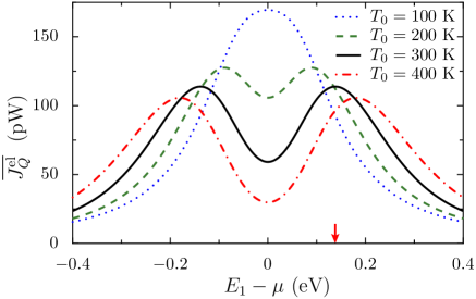
Figure 2: (Color online) Directed electronic heat current $\overline{J^{\text{el}}_{Q}}$ as function of onsite energy $E_{1}-\mu$ for different reference temperatures $T_{0}$ and temperature oscillation amplitude $A=30$ K. The arrow marks the onsite energy $E_{1}-\mu=0.138$ eV for which the pumped electron current assumes at temperature $T_{0}=300$ K its maximum. The adiabatic rocking frequency is $\Omega=3.92$ GHz.

III Pumping heat via single-sided temperature rocking

Let us first consider the case in which the temperature of one lead is modulated sinusoidally, while the temperature of the other lead is constant,

$$T_{\text{L}}(t) =T_{0}+A\cos(\Omega t),$$ (19)

$$T_{\text{R}}(t) =T_{0}.$$

Here $A$ and $\Omega$ are the driving amplitude and (angular) frequency of the temperature modulation, respectively, while $T_{0}$ is the reference temperature. The driving amplitude $A$ is positive and bounded by the temperature $T_{0}$ since $T_{\text{L}}(t)$ has to remain positive at any time. The temperature difference between left and right lead reads $\Delta T(t)=A\cos(\Omega t)$, such that the net thermal bias vanishes on time-average, $\overline{\Delta T(t)}=0$.

The cycle-averaged heat fluxes, both the electronic and the phononic one, follow from numerically evaluating the integrals in Eqs. (12) and (13). As expected for an adiabatic theory, we observe that the average heat current $\overline{J_{Q}}$ is independent of the driving frequency $\Omega$. This is in accordance with the findings for ballistic heat transfer in the adiabatic regime.

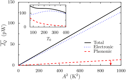
Figure 3: (Color online) Total electronic and phononic time-averaged, directed heat current $\overline{J_{Q}}$ as function of the squared driving amplitude $A^{2}$ with reference temperature at $T_{0}=300$ K for the onsite energy $E_{1}-\mu=0.138$ eV. The dotted line represents the electronic contribution, the dashed line the phononic one. The inset depicts the directed heat current as a function of the reference temperature $T_{0}$ for the amplitude $A=30$ K ($A^{2}=900\,\mathrm{K}^{2}$) marked by the arrow in the main panel.

In an experiment, the molecular level $E_{1}$ can be manipulated by a gate voltage which influences only the electrons. This allows one to tune the electron transport while keeping the phonons untouched. In Fig. 2, we depict the net electron heat current $\overline{J^{\text{el}}_{Q}}$ as a function of $E_{1}-\mu$ for a fixed driving amplitude. We find that the heat current possesses an extremum for $E_{1}-\mu=0$, i.e., when the onsite energy is aligned with the Fermi energy. Interestingly enough, this extremum is a maximum for low reference temperature $T_{0}$ and turns into a minimum when the temperature exceeds a certain values. This implies that the net electron heat current is rather sensitive to the on-site energy with respect to the Fermi energy. This property thus provides an efficient way to determine experimentally the Fermi energy of the wire as an alternative to, e.g., measuring the thermopower as proposed in Ref. datta2003 . For large gate variations we find that the directed electron heat current is significantly suppressed since the wire level is far off the electron thermal energy, i.e., $E_{1}-\mu\gg k_{\text{B}}T_{0}$. The directed heat current then is dominated by the phonon heat flux. As temperature is increased, the peak positions of the pumped electron heat current shifts outwards, away from the Fermi energy. At room temperature $T=300$ K, the peak positions are located at $E_{1}-\mu=\pm\,0.138$ eV.

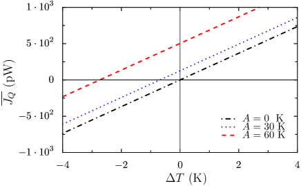
Figure 4: (Color online) Total directed heat current $\overline{J_{Q}}$ as the function of static thermal bias $\Delta T$ for different driving amplitude strengths $A$ for the temperature modulation. The reference temperature is set as $T_{0}=300$ K and the electronic wire level is set as $E_{1}-\mu=0.138$ eV.

III.1 Scaling behavior for small driving strengths

Figure 3 shows the total heat current $\overline{J_{Q}}$ as a function of the driving amplitude $A$ for the reference temperature $T_{0}=300$ K and the electronic site above the Fermi level. For weak driving ($A\ll T_{0}$), we find $\overline{J^{\text{el}(\text{ph})}_{Q}}\propto A^{2}$ for both the electronic and the phononic contribution. This behavior can be understood from a Taylor expansion of the Fermi-Dirac and the Bose-Einstein distribution,

$$\begin{split}g(&\xi,T_{\text{L}})-g(\xi,T_{0})\\ &=g(\xi,T_{0}+\Delta T)-g(\xi,T_{0})\\ &=g^{\prime}(\xi,T_{0})\Delta T(t)+\frac{g^{\prime\prime}(\xi,T_{0})}{2}[\Delta T(t)]^{2}+\cdots\,,\end{split}$$ (20)

where $g$ represents the Fermi-Dirac function $f$ and the Bose-Einstein function $n$, while $g^{\prime}$ and $g^{\prime\prime}$ denote derivatives with respect to temperature. Note that the time-dependence stems solely from the temperature difference $\Delta T(t)$. After a cycle average over the driving period, the first term in the expansion vanishes owing to $\overline{\Delta T(t)}=0$. Therefore, the leading term of the heat current is of second order, i.e. $\propto\overline{[\Delta T(t)]^{2}}$, which yields $\overline{J^{\text{el}(\text{ph})}_{Q}}\propto\int^{2\pi/\Omega}_{0}[\Delta T(t)]^{2}dt\propto A^{2}$, as observed numerically. We also plot the directed heat current as the function of the reference temperature $T_{0}$ in the inset of Fig. 3: The directed phonon heat current decreases monotonically upon increasing the reference temperature. However, the emerging total heat current exhibits a relatively flat behavior in a large temperature range. This is due to the combined effect from phonons and electrons. At high temperatures, the electron heat flux dominates the overall directed heat flow.

III.2 Thermal load characteristics and ratchet-induced thermoelectric voltage

Thus far we have studied heat pumping in the absence of a static temperature bias, i.e. for $\overline{\Delta T(t)}=0$. We next introduce a static thermal bias such that a thermal bias $\Delta T:=\overline{\Delta T(t)}\neq 0$ emerges. The resulting total directed heat current $\overline{J_{Q}}$ is depicted in Fig. 4. Within this load curve, we spot a regime with negative static thermal bias $\Delta T<0$ and positive-valued overall heat flow until $\Delta T$ reaches the stop-bias value, i.e., we find a so-called Brownian heat-ratchet effect BHM1 ; BHM2 . This means that heat can be directed against a thermal bias from cold to warm like in a conventional heat pump. The width of this regime scales with the driving amplitude $A^{2}$, cf. Fig. 4.

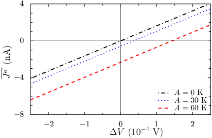
Figure 5: (Color online) The time-averaged directed electric current $\overline{J^{\text{el}}}$ as function of the static voltage bias $\Delta V$ for different temperature amplitudes $A$. The reference temperature is $T_{0}=300$ K and the electronic wire level is at $E_{1}-\mu=0.138$ eV.

As can be deduced from Fig. 4, a zero-biased temperature modulation generates a finite net heat flow at zero temperature bias similar to the heat flow that would be induced by a static thermal bias.

Near equilibrium, i.e. within the linear response regime, Onsager symmetry relations for transport of conjugated quantities are expected to hold. Therefore, the adiabatic temperature modulations are expected to induce an electric current as well. This net adiabatic electric pump current can be obtained by means of the cycle-averaged Landauer expression which reads explicitly:

$$\overline{J^{\text{el}}}=\frac{\Omega}{2\pi}\int_{0}^{2\pi/\Omega}dt\frac{e}{h}\int d\varepsilon\,\mathcal{T}(\varepsilon)\left[f(\varepsilon,T_{\text{L}})-f(\varepsilon,T_{\text{R}})\right].$$ (21)

We in addition apply a net static voltage bias $\Delta V$. Figure 5 depicts the net electric current-voltage characteristics $\overline{J^{\text{el}}}(\Delta V)$ in the presence of an unbiased temperature modulation while, importantly no external thermal bias is applied. For a positive bias voltage $\Delta V>0$, the net electric current is negative, i.e. the system effectively acts as an “electron pump”.

The value of this externally applied electric stop-voltage $\Delta V_{\text{st}}$, which renders the electric current vanishing, mimics here a sole heat-ratchet induced thermopower. In the present context, this constitutes a novel phenomenon which we term ratchet Seebeck effect. Knowingly, the usual thermopower (Seebeck coefficient) is defined by means of the change in induced voltage per unit change in applied temperature bias under conditions of zero electric current callen . Here, in the absence of a net thermal bias, we introduce instead a Grüneisen-like relation, reading $\gamma=|\Delta V_{\text{eff}}/\overline{J^{\text{el}}}|$, where $\Delta V_{\text{eff}}$ denotes the effective static voltage bias which yields the identical electric heat current $\overline{J^{\text{el}}}$ as generated by our imposed temperature modulation. It is found that this effective voltage bias precisely matches the above mentioned stop-voltage, i.e. $\Delta V_{\text{eff}}=\Delta V_{\text{st}}$. Due to the linear $\overline{J^{\text{el}}}$–$\Delta V$ characteristics, as evidenced with Fig. 5, the Grüneisen-like constant $\gamma$ is independent of the amplitude of the temperature modulation. In doing so, we find for $T_{0}=300$ K and $E_{1}-\mu=0.138$ eV, that this very Grüneisen-like constant becomes $\gamma=61.9\times 10^{3}\mathrm{V/A}$.

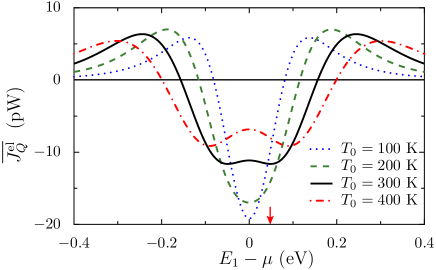
Figure 6: (Color online) Directed electron heat current $\overline{J^{\text{el}}_{Q}}$ as function of the wire level $E_{1}-\mu$ for various reference temperatures $T_{0}$. The driving parameters are $A_{1}=A_{2}=30$ K and $\varphi=0$.

IV Temperature rocking in both leads: Pumping heat by dynamical symmetry breaking

We next consider temperature modulations applied to both leads in the absence of a thermal bias. The temperature driving consists of a contribution with frequency $\Omega$ and a second harmonic with frequency $2\Omega$. This entails a dynamical symmetry breaking, namely harmonic mixing SB1 ; SB2 ; SB3 ; SB4 ; SB5 . The time-dependent lead temperatures are chosen as

$$T_{\text{\text{L},\text{R}}} =T_{0}\pm[A_{1}\cos(\Omega t)-A_{2}\cos(2\Omega t+\varphi)],$$ (22)

such that again $\overline{T_{\text{L}}(t)}=\overline{T_{\text{R}}(t)}=T_{0}$ and $\Delta T(t)=2[A_{1}\cos(\Omega t)+A_{2}\cos(2\Omega t+\varphi)]$. Then the average temperature bias vanishes irrespective of the phase lag $\varphi$.

In Fig. 6, we depict the resulting electron heat current $\overline{J^{\text{el}}_{Q}}$ as a function of the on-site energy $E_{1}-\mu$ for various reference temperatures $T_{0}$. At low temperatures, the net electron heat current exhibits a minimum at the Fermi energy. With increasing reference temperature $T_{0}$ this minimum then develops into a local maximum with two local minima in its vicinity. The arrow in Fig. 6 marks the minimum at $E_{1}-\mu=0.049$ eV for $T_{0}=300$ K. It is interesting that the direction of the net electron heat current can be tuned by the gate variation. For an electron wire level close to the Fermi energy, the directed electron heat current is negative. By tuning the gate voltage, the heat current undergoes a reversal and becomes positive when $E_{1}-\mu$ is larger than $0.15$ eV (at reference temperature $T_{0}=300$ K) and eventually approaches zero again for large detuning.

Figure 7 shows the corresponding sum of electron and phonon heat flow, i.e., the net heat current $\overline{J_{Q}}$ as a function of wire level $E_{1}-\mu$. The net phonon heat current $\overline{J^{\text{ph}}_{Q}}$ is negative for these parameters (not depicted) and is not sensitive to the gate voltage. As a consequence, this sum of phonon and electron heat transport, $\overline{J_{Q}}$, exhibits multiple current reversals as the onsite energy $E_{1}-\mu$ increases. For small values of $E_{1}-\mu$, i.e., close to the Fermi surface, both the electron and the phonon heat fluxes are negative and in phase with the driving. The absolute value of the total heat current assumes its maximum (at which the heat current is negative). For intermediate values of $E_{1}-\mu$, the direction of total net current $\overline{J_{Q}}$ is reversed due to the dominating positive contribution of the electrons. At even larger values of $E_{1}-\mu$, the electron heat current almost vanishes, so that the total heat current is dominated by the negative-valued contribution of the phonons. In the limit of large $E_{1}-\mu$, we find saturation at a negative value.

Figure 7: Total net heat current $\overline{J_{Q}}$ as function of the wire level $E_{1}-\mu$ for reference temperature $T_{0}=300$ K, amplitudes $A_{1}=A_{2}=30$ K, and phase lag $\varphi=0$.

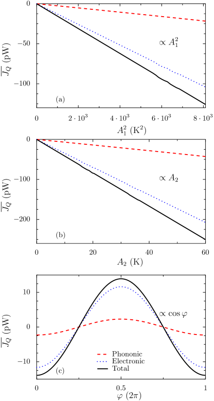
Figure 8: (Color online) Heat current $\overline{J_{Q}}$ as function of (a) fundamental driving strength $A_{1}$, where $A_{2}=30$ K and $\varphi=0$ and (b) as function of the second-harmonic amplitude $A_{2}$, where $A_{1}=90$ K and $\varphi=0$. (c) Dependence on the relative phase $\varphi$ for $A_{1}=A_{2}=30$ K. The reference temperature is $T_{0}=300$ K, while the wire level is $E_{1}-\mu=0.049$ eV.

We also study with Fig. 8 the net electron and phonon heat current as the function of driving amplitudes $A_{1}$, $A_{2}$ and the relative phase $\varphi$. Both contributions scale as $\overline{J^{\text{el}/\text{ph}}_{Q}}\propto A_{1}^{2}A_{2}\cos(\varphi)$, which implies that they can be manipulated simultaneously. This behavior can be understood by again expanding the Fermi-Dirac and the Bose-Einstein function at $T_{0}$:

$$\begin{split}g(\xi,&T_{\text{L}})-g(\xi,T_{\text{R}})\\ &=g(\xi,T_{0}+\Delta T/2)-g(\xi,T_{0}-\Delta T/2)\\ &=g^{\prime}(\xi,T_{0})\Delta T(t)+\frac{g^{\prime\prime\prime}(\xi,T_{0})}{24}[\Delta T(t)]^{3}+\cdots,\end{split}$$ (23)

where $g=f,n$ represents the distribution function for the electrons and for the phonons, respectively. Note that the terms of even order in $\Delta T$ vanish owing to the anti-symmetric temperature modulation. Thus, the heat currents are governed by the time-average of the odd powers $[\Delta T(t)]^{2n+1}$ with $n>1$, since $\overline{\Delta T}=0$. It can be easily verified that all these time-averaged odd moments vanish if either amplitude, $A_{1}$ or $A_{2}$ vanishes. Note that the lowest lowest-order contribution is the third moment $\overline{[\Delta T(t)]^{3}}=8A_{1}^{2}A_{2}\cos(\varphi)$. Thus, for small driving amplitudes, $A_{1},A_{2}\ll T_{0}$, the net electron and phonon heat current are expected to be proportional to $A_{1}^{2}A_{2}\cos\varphi$ as is corroborated with the numerical results depicted in Figs. 8(a,b,c). This proportionality to $\cos\varphi$, see Fig. 8(c), is even more robust than a priori expected; this is so because the cycle averaged 5-th and 7-th moment are proportional to $\varphi$, as well, i.e., $\overline{[\Delta T(t)]^{5}},\overline{[\Delta T(t)]^{7}}\propto\cos(\varphi)$. This behavior can be employed for a sensitive control of the heat current: The direction of the heat current can be reversed by merely adjusting the relative phase $\varphi$ between the two harmonics. Note that for the parameters used in the figure, the net electron heat current $\overline{J^{\text{el}}_{Q}}$ exceeds the net phonon heat current $\overline{J^{\text{ph}}_{Q}}$ roughly by a factor $5$.

V Conclusions

We have demonstrated the possibility of steering heat across a gated two-terminal molecular junction, owing to lead temperatures that undergo adiabatic, unbiased, time-periodic modulations. In a realistic molecule, the heat flow is carried by the electrons as well as by the phonons. Our study considers both contributions. Two scenarios of temperature modulations have been investigated, namely directed heat flow (i) induced by periodic temperature manipulation in one connecting lead and (ii) created by a temperature modulation that includes a contribution oscillating with twice the fundamental frequency. In both cases, we predict a finite heat current which is related to dynamical breaking of reflection symmetry. A necessary ingredient is the non-linearity of the initial electron and phonon distribution, which is manifest in the Fermi-Dirac distribution and the Bose-Einstein distribution. The first scenario yields sizable heat currents proportional to the squared amplitude of the temperature modulation. The resulting heat flow occurs in the absence of a static thermal bias. We also studied heat pumping against an external static thermal bias and computed the corresponding thermal heat-current load characteristics. Moreover, the ratchet heat flow in turn generates also an electric current. This ratchet heat current induces a novel phenomenon, namely a ratchet-induced, effective thermopower, see in Fig. 5.

When the asymmetry is induced by temperature rocking at both leads, the resulting net heat current becomes smaller in size. This is so because the leading-order time-averaged heat flow now starts out with the third moment of the driving amplitude. The benefit of this second scenario is the possibility of controlling efficiently both the magnitude and the sign of the net heat flow. For example, the direction of the heat current can be readily reversed via the gate voltage or the relative phase between two temperature modulations that are harmonically mixed. When adjusting the gate voltage, the directed heat current experiences multiple current reversals. The directed heat flow is even up to 7-th order in the amplitude proportional to the cosine of the phase between the fundamental frequency and the second harmonic. This allows robust control even for relatively large temperature amplitudes.

These theoretical findings may also inspire experimental efforts to steer heat in a controlled manner across a molecular junction as well as the development of new concepts for measuring system parameters via their impact on the heat current. For example, as elucidated in Sect. III, the Fermi energy can be sensitively gauged in this way.

Appendix A The derivation of phonon transmission (18)

We derive the phonon transmission coefficient of Eq. (18) along the lines of Ref. segal . Starting with Eq. (33) of that work and assuming symmetric coupling, i.e. $\gamma^{\text{L}}_{k,k^{\prime}}(\omega_{0})=\gamma^{\text{R}}_{k,k^{\prime}}(\omega_{0})=\gamma_{k,k^{\prime}}(\omega_{0})$, Eq. (33) of Ref. segal can be simplified to read

$$\begin{split}&[\omega^{2}_{k}-\omega^{2}_{0}+2i\omega_{0}\gamma_{k,k}(\omega_{0})]A_{k}(\omega_{0})\\ &+i\omega_{0}\sum_{k^{\prime}\neq k}\sqrt{\frac{\omega_{k}}{\omega_{k^{\prime}}}}2\gamma_{k,k^{\prime}}(\omega_{0})A_{k^{\prime}}(\omega_{0})=\sqrt{\frac{\omega_{k}}{\omega_{0}}}V_{0,k}a^{\dagger}_{0},\end{split}$$ (24)

where $\omega_{0}$ is a dummy variable.

Since we only consider one phonon mode, i.e. $k=1$. The second term in the left hand side of last equation vanishes such that

$$[\omega^{2}_{1}-\omega^{2}_{0}+2i\omega_{0}\gamma_{1,1}(\omega_{0})]A_{1}(\omega_{0})=\sqrt{\frac{\omega_{1}}{\omega_{0}}}V_{0,1}a^{\dagger}_{0}.$$ (25)

Substituting Eq. (46) of Ref. segal , i.e.

$$A_{k}(\omega_{0})=\overline{A_{k}}(\omega_{0})V_{0,k}a^{\dagger}_{0}\sqrt{\frac{\omega_{k}}{\omega_{0}}}$$ (26)

into Eq. (25), we find

$$\overline{A_{1}}(\omega_{0})=\frac{1}{\omega^{2}_{1}-\omega^{2}_{0}+2i\omega_{0}\gamma_{1,1}(\omega_{0})}$$ (27)

For one phonon mode, the phonon transmission is defined from Eq. (48) in segal . However, this definition is $1/2\pi$ times smaller than the commonly used definition of Ref. rego and jswang . With the commonly used definition, the phonon transmission can be expressed as

$$\mathcal{T}(\omega)=4\omega^{2}\gamma^{2}_{1,1}(\omega)|\overline{A_{1}}(\omega)|^{2}.$$ (28)

Substituting Eq. (27) into the last equation and omitting the subscript in $\gamma_{1,1}$, we obtain

$$\mathcal{T}(\omega)=\frac{4\omega^{2}\gamma^{2}(\omega)}{(\omega^{2}_{1}-\omega^{2})^{2}+4\omega^{2}\gamma^{2}(\omega)}$$ (29)

which is the phonon transmission (18) employed in the main text.

References

- (1) A. Nitzan and M. A. Ratner, Science 300, 1384 (2003).
- (2) Molecular Nanoelectronics, ed. by M. A. Reed and T. Lee (American Scientific Publishers, Stevenson Ranch, CA, 2003).
- (3) P. Hänggi, M. Ratner, and S. Yaliraki, Chem. Phys. 281, 111 (2002).
- (4) S. Kohler, J. Lehmann, and P. Hänggi, Phys. Rep. 406, 379 (2005).
- (5) N. J. Tao, Nature Nanotechnology, 1, 173 (2006).
- (6) M. A. Reed and J. M. Tour, Sci. Am. (Int. Ed.) 282, 86 (2000).
- (7) P. J. Kuekes, D. R. Stewart, and R. S. Williams, J. Appl. Phys. 97, 034031 (2005).
- (8) C. Zhang, M.-H. Du, H.-P. Cheng, X.-G. Zhang, A. E. Roitberg, and J. L. Krause, Phys. Rev. Lett. 92, 158301 (2004).
- (9) J. Lehmann, S. Camalet, S. Kohler, and P. Hänggi, Chem. Phys. Lett. 368, 282 (2003).
- (10) J. Lehmann, S. Kohler, V. May, and P. Hänggi, J. Chem. Phys. 121, 2278 (2004).
- (11) G.-Q. Li, M. Schreiber, and U. Kleinekathöfer, EPL 79, 27006 (2007).
- (12) I. Franco, M. Shapiro, and P. Brumer, Phys. Rev. Lett. 99, 126802 (2007).
- (13) S. Kohler and P. Hänggi, Nature Nanotechnology 2, 675 (2007).
- (14) Z. Q. Yang, N. D. Lang, and M. Di Ventra, Appl. Phys. Lett. 82, 1938 (2003).
- (15) A. Ghosh, T. Rakshit, and S. Datta, Nano Lett. 4, 565 (2004).
- (16) F. Jiang, Y. X. Zhou, H. Chen, R. Note, H. Mizuseki, and Y. Kawazoe, J. Chem. Phys. 125, 084710 (2006).
- (17) K. Xiao, Y. Liu, T. Qi, W. Zhang, F. Wang, J. Gao, W. Qiu, Y. Ma, G. Cui, S. Chen, X. Zhan, G. Yu, J. Qin, W. Hu, and D. Zhu, J. Am. Chem. Soc. 127, 13181 (2005).
- (18) Y. Sun, Y. Liu, and D. Zhu, J. Mater. Chem 15, 53 (2005).
- (19) B. Xu, X. Xiao, X. Yang, L. Zang, and N. Tao, J. Am. Chem. Soc. 127, 2386 (2005).
- (20) L. Wang and B. Li, Phys. World 21, 27 (2008).
- (21) M. Terraneo, M. Peyrard, and G. Casati, Phys. Rev. Lett. 88, 094302 (2002).
- (22) B. Li, L. Wang, and G. Casati, Phys. Rev. Lett. 93, 184301 (2004).
- (23) D. Segal and A. Nitzan, Phys. Rev. Lett. 94, 034301 (2005).
- (24) B. Hu, L. Yang, and Y. Zhang, Phys. Rev. Lett. 97, 124302 (2006).
- (25) M. Peyrard, Europhys. Lett. 76, 49 (2006).
- (26) N. Yang, N. Li, L. Wang, and B. Li, Phys. Rev. B 76, 020301(R) (2007).
- (27) D. Segal, Phys. Rev. Lett. 100, 105901 (2008).
- (28) B. Li, L. Wang, and G. Casati, Appl. Phys. Lett. 88, 143501 (2006).
- (29) W. C. Lo, L. Wang, and B. Li, J. Phys. Soc. Jpn. 77, 054402 (2008).
- (30) L. Wang and B. Li, Phys. Rev. Lett. 99, 177208 (2007).
- (31) L. Wang and B. Li, Phys. Rev. Lett. 101, 267203 (2008).
- (32) C. W. Chang, D. Okawa, A. Majumdar, and A. Zettl, Science 314, 1121 (2006).
- (33) R. Scheibner, M. König, D. Reuter, A. D. Wieck, C. Gould, H. Buhmann, and L. W. Molenkamp, New J. Phys. 10, 083016 (2008).
- (34) P. Reimann, R. Bartussek, R. Häussler, and P. Hänggi, Phys. Lett. A 215, 26 (1996).
- (35) R. D. Astumian and P. Hänggi, Phys. Today 55 (11), 33 (2002).
- (36) P. Hänggi, F. Marchesoni, and F. Nori, Ann. Phys. (Leipzig) 14, 51 (2005).
- (37) P. Reimann and P. Hänggi, Appl. Phys. A 75, 169 (2002).
- (38) P. Hänggi and F. Marchesoni, Rev. Mod. Phys. 81, 387 (2009).
- (39) N. Li, P. Hänggi, and B. Li, EPL 84, 40009 (2008).
- (40) N. Li, F. Zhan, P. Hänggi, and B. Li, Phys. Rev. E 80, 011125 (2009).
- (41) M. Rey, M. Strass, S. Kohler, P. Hänggi, and F. Sols, Phys. Rev. B 76, 085337 (2007).
- (42) L. Arrachea, M. Moskalets, and L. Martin-Moreno, Phys. Rev. B 75, 245420 (2007).
- (43) J. Luczka, R. Bartussek, and P. Hänggi, Europhys. Lett. 31, 431 (1995).
- (44) P. Hänggi, R. Bartussek, P. Talkner, and J. Luczka, Europhys. Lett. 35, 315 (1996).
- (45) I. Goychuk and P. Hänggi, Europhys. Lett. 43, 503 (1998).
- (46) S. Flach, O. Yevtushenko, and Y. Zolotaryuk, Phys. Rev. Lett. 84, 2358 (2000).
- (47) S. Denisov, S. Flach, A. A. Ovchinnikov, O. Yevtushenko, and Y. Zolotaryuk, Phys. Rev. E 66, 041104 (2002).
- (48) M. Galperin, M. A. Ratner, and A. Nitzan, J. Phys.: Condens. Matter 19, 103201 (2007).
- (49) D. Segal and A. Nitzan, J. Chem. Phys. 122, 194704 (2005).
- (50) D. Segal, Phys. Rev. B 73, 205415 (2006).
- (51) U. Sivan and Y. Imry, Phys. Rev. B 33, 551 (1986).
- (52) X. Zheng, W. Zheng, Y. Wei, Z. Zeng, and J. Wang, J. Chem. Phys. 121, 8537 (2004).
- (53) L. G. C. Rego and G. Kirczenow, Phys. Rev. Lett. 81, 232 (1998).
- (54) A. Ozpineci and S. Ciraci, Phys. Rev. B 63, 125415 (2001).
- (55) D. Segal, A. Nitzan, and P. Hänggi, J. Chem. Phys. 119, 6840 (2003).
- (56) J.-S. Wang, J. Wang, and J. T. Lü, Eur. Phys. J. B 62, 381 (2008).
- (57) J. Lee, A. O. Govorov, and N. A. Kotov, Angew. Chem. Inter. Ed., 44, 7439 (2005).
- (58) R. H. M. Groeneveld, R. Sprik, and A. Lagendijk, Phys. Rev. B 51, 11433 (1995).
- (59) N. Del Fatti, C. Voisin, M. Achermann, S. Tzortzakis, D. Christofilos, and F. Valleé, Phys. Rev. B 61, 16956 (2000).
- (60) R. Knorren, K. H. Bennemann, R. Burgermeister, and M. Aeschlimann, Phys. Rev. B 61, 9427.
- (61) P. J. van Hall, Phys. Rev. B 63, 104301 (2001).
- (62) J. P. Girardeau-Montaut, M. Afif, C. Girardeau-Montaut, S. D. Moustaïzis, and N. Papadogiannis, App. Phys. A 62, 3 (1996).
- (63) M. van Kampen, J. T. Kohlhepp, W. de Jonge, B. Koopmans, and R. Coehoorn, J. Phys.: Condens. Matter 17, 6823 (2005).
- (64) M. Paulsson and S. Datta, Phys. Rev. B 67, 241403(R) (2003).
- (65) J. Grunenberg, Angew. Chem. Int. Ed. 40, 4027 (2001).
- (66) Z. Wang, J. A. Carter, A. Lagutchev, Y. K. Koh, N. Seong, D. G. Cahill, and D. D. Dlott, Science 317, 787 (2007).
- (67) H. B. Callen, Thermodynamics and an Introduction to Thermostatics, 2-nd edition, (Wiley, New York, 1985), see Sects. 14.5-14.9 therein.