Nonlinear Evolution of Axisymmetric Twisted Flux Tubes in the Solar Tachocline

Abstract

We numerically study the evolution of magnetic fields and fluid flows in a thin spherical shell. We take the initial field to be a latitudinally confined, predominantly toroidal flux tube. For purely toroidal, untwisted flux tubes, we recover previously known radial-shredding instabilities, and show further that in the nonlinear regime these instabilities can very effectively destroy the original field. For twisted flux tubes, including also a poloidal component, there are several possibilities, including the suppression of the radial-shredding instability, but also a more directly induced evolution, brought about because twisted flux tubes in general are not equilibrium solutions of the governing equations.

1 Introduction

The solar tachocline is the transition zone between the uniformly rotating radiative interior and the differentially rotating convection zone. First discovered helioseismically in the early 1990s, it continues to be probed to this day. Of particular interest is how thin it is; the angular-velocity profile changes dramatically over no more than about 5% of the solar radius. This intense shear is one of the reasons why the tachocline is now generally believed to be the seat of the solar dynamo, with poloidal fields being sheared out to produce very strong toroidal fields. Seehrw07for reviews of many different aspects of the tachocline, including its role in the solar dynamo.

Given the combination of strong magnetic fields and shear, it was quickly realized that so-called magneto-shear instabilities could potentially play an important role in the dynamics of the tachocline. Indeed, in other contexts, long before the tachocline was even discovered, it had been known that both magnetic fields [Gough and Tayler (1966)] and shear [Watson (1981)] separately can lead to instabilities. The first to study this problem in the tachocline context weregilfox97; one very interesting result that they obtained was that a combination of magnetic fields and shear can be unstable even though each ingredient separately would be stable. Gilman and Fox carried out a 2D calculation, confined to the surface of a sphere, with no radial variations allowed. Subsequent work extended this to quasi-3D shallow-water and 3D thin-shell models, including also both linear onset and nonlinear equilibration studies. Seegc07for a review of this work.

We will consider a different type of two-dimensionality, namely axisymmetric solutions. These have not received as much attention as some of the 3D solutions, but recent linear-onset calculations Cally, Dikpati, and Gilman (2008); Dikpati et al. (2009) indicate that if the toroidal field is concentrated into latitudinal bands, instabilities may arise that shred the field in the radial direction. In this paper we consider the nonlinear evolution of such banded fields. For purely toroidal, untwisted flux tubes, we obtain results in good qualitative agreement with the linear-onset calculations. For mixed toroidal plus poloidal, twisted flux tubes (which were not considered before) we show that the field evolves not just via the onset of instabilities, but much more directly, simply because in general it is not an equilibrium solution of the governing equations. For twisted flux tubes there is then a variety of possible outcomes, depending on the strengths of both the toroidal and poloidal components.

2 Equations

sec:equations

The equations we wish to solve are the (Boussinesq) Navier-Stokes equation

$$\frac{\partial{\bf v}}{\partial t}+{\bf v\cdot\nabla v}=-\nabla p+{\bf(\nabla\times a)\times a}+S{\bf\hat{e}}_{r}+\epsilon\nabla^{2}{\bf v},$$

the magnetic induction equation

$$\frac{\partial{\bf a}}{\partial t}=\nabla\times({\bf v\times a})+\epsilon\nabla^{2}{\bf a},$$

and the entropy equation

$$\frac{\partial S}{\partial t}+{\bf v}\cdot\nabla S=-N^{2}{\bf v\cdot\hat{e}}_{r}+\epsilon\nabla^{2}S.$$

Here $\bf v$ and $\bf a$ denote the fluid and Alfvén velocities, respectively, and $S$ the entropy. $N$ is the Brunt-Väisälä frequency, assumed constant. Length has been scaled by the inner edge of the tachocline, so we will be interested in solving this system in the interval $r\in[1,1.05]$. Time has been scaled by the equatorial rotation frequency, $\bf v$ and $\bf a$ as length/time.

Except for the inclusion of the diffusive terms $(\epsilon\nabla^{2}\cdot)$, these equations are the same as incdg08, hereafter referred to as CDG08. Some diffusivity must be included here to ensure numerical stability, but values in the range $\epsilon=10^{-5}$ to $10^{-6}$ yielded similar results, indicating that diffusivity is not significantly affecting the evolution. The results presented here are all at $\epsilon=2\times 10^{-6}$.

While the equations may be much the same, the subsequent analysis is very different from that of CDG08. They considered only the linear onset of instability, and only for high radial wavenumber $(k)$, thereby ultimately eliminating $r$ entirely, instead simply having $k$ as a parameter in the equations. In contrast, we are interested in a direct numerical solution, in the finite interval $r\in[1,1.05]$, allowing an arbitrary radial dependence, and including also the full nonlinear evolution of the solutions.

For axisymmetric solutions, it is convenient to decompose $\bf v$ and $\bf a$ as

$${\bf v}=v{\bf\hat{e}}_{\phi}+\nabla\times(\psi{\bf\hat{e}}_{\phi}),\qquad{\bf a}=b{\bf\hat{e}}_{\phi}+\nabla\times(a{\bf\hat{e}}_{\phi}).$$

The toroidal parts, $v$ and $b$, are the azimuthal components of the given vectors; the poloidal parts, $\psi$ and $a$, are the streamfunctions of the meridional components. The original Equations (1) and (2) then become

$$\frac{\partial}{\partial t}v=P_{1}(b,a)-P_{1}(v,\psi)+\epsilon D^{2}v,$$

$$\frac{\partial}{\partial t}D^{2}\psi=\frac{1}{r}\frac{\partial}{\partial\theta}S+P_{2}(b,b)+P_{2}(D^{2}a,a)-P_{2}(v,v)-P_{2}(D^{2}\psi,\psi)+\epsilon D^{4}\psi,$$

$$\frac{\partial}{\partial t}b=P_{2}(v,a)-P_{2}(b,\psi)+\epsilon D^{2}b,$$

$$\frac{\partial}{\partial t}a=P_{1}(\psi,a)+\epsilon D^{2}a,$$

where

$$D^{2}=\nabla^{2}-1/(r\sin\theta)^{2},$$

and

$$P_{1}(X,Y)={\bf\hat{e}}_{\phi}\cdot\bigl{[}\bigl{(}\nabla\times(X{\bf\hat{e}}_{\phi})\bigr{)}\times\bigl{(}\nabla\times(Y{\bf\hat{e}}_{\phi})\bigr{)}\bigr{]},$$

$$P_{2}(X,Y)={\bf\hat{e}}_{\phi}\cdot\nabla\times\bigl{[}(X{\bf\hat{e}}_{\phi})\ \times\bigl{(}\nabla\times(Y{\bf\hat{e}}_{\phi})\bigr{)}\bigr{]}.$$

We then wish to solve (5) and (6), with stress-free boundary conditions

$$\frac{\partial}{\partial r}\Bigl{(}\frac{v}{r}\Bigr{)}=\psi=\frac{\partial^{2}}{\partial r^{2}}\psi=0\qquad{\rm at}\quad r=1,1.05,$$

(7) and (8), with perfectly conducting boundary conditions

$$\frac{\partial}{\partial r}\bigl{(}br\bigr{)}=a=0\qquad{\rm at}\quad r=1,1.05,$$

and (3), with $S=0$ at $r=1,1.05$. These boundary conditions are somewhat artificial, but any boundary conditions would necessarily be artificial. To properly capture all of the dynamics of the tachocline, it should not be studied in isolation, but rather as part of a global model that also includes the interior and the convection zone. However, while there are models that aim in this direction Brun and Toomre (2002), they are so complicated that one cannot focus specifically on aspects such as tachocline instabilities. To study tachocline instabilities, one must therefore adopt simplified models such as ours, despite the inevitably unnatural boundaries where the real Sun has none.

We solve these equations using the numerical code described byh2000, in which the radial structure is expanded in terms of Chebyshev polynomials, the angular structure in terms of spherical harmonics, and the time-stepping is done via a second-order Runge-Kutta method. Resolutions ranging from $50\times 1600$ to $80\times 2400$ in $(r,\theta)$ were used, and were all checked to ensure that the results were adequately resolved. A timestep of $10^{-3}$ was sufficiently small to ensure stability.

To facilitate comparison with CDG08, we choose initial conditions much the same as theirs. The initial entropy is simply $S=0$, so any buoyancy effects arise entirely out of the subsequent evolution. For the flow, we take the solar-like differential rotation profile $\omega=v/(r\sin\theta)=1-0.18\cos^{2}\theta$, where we note that (1) is written in a non-rotating frame, so $\omega$ here must include an overall rotation, not just the Pole-to-Equator differential rotation $-0.18\cos^{2}\theta$.

For the toroidal field, we take

$$b=Ap\bigl{[}{\mathrm{e}}^{-4(\mu-d)^{2}/W^{2}(1-d^{2})}-{\mathrm{e}}^{-4(\mu+d)^{2}/W^{2}(1-d^{2})}\bigr{]}\sin\theta/r,$$

where $\mu=\cos\theta$. That is, $b$ consists of two oppositely directed bands in the two hemispheres, with position $d$, latitudinal bandwidth $W$, and amplitude $A$. The normalization factor $p$ is adjusted such that the maximum field strength $\max_{\theta}(b)$ is $A/2$.

Values of $A$ up to one, corresponding in dimensional terms to $\max_{\theta}(b)\approx 10^{5}$ G, are of greatest interest in the solar context, but other (especially younger) solar-type stars may well have even larger values. We will present runs for $A=1$ and $2$. A range of possibilities for $d$ and $W$ were considered, and yielded qualitatively similar results. We therefore show results only for $d=0.5$, corresponding to bands situated $\pm 30^{o}$ from the Equator, and $W=\pi/36$, corresponding to a bandwidth of $5^{o}$.

Thus far our initial conditions are exactly as in CDG08; see alsodg99, who were the first to introduce banded toroidal fields of this type. To this toroidal field, we now add the poloidal field

$$a=A^{\prime}p^{\prime}\bigl{[}{\mathrm{e}}^{-4(\mu-d)^{2}/W^{2}(1-d^{2})}+{\mathrm{e}}^{-4(\mu+d)^{2}/W^{2}(1-d^{2})}\bigr{]}\sin\theta(r-1)(r-1.05).$$

The poloidal field thus has the same banded structure as the toroidal, but $a$ is equatorially symmetric, whereas $b$ is anti-symmetric. Both of these symmetries correspond to the standard “dipole” solutions of solar dynamo theory. The differing radial dependencies, $(r-1)(r-1.05)$ for $a$ versus $1/r$ for $b$, are dictated by the different boundary conditions (13) that $a$ and $b$ are supposed to satisfy. The normalization factor $p^{\prime}$ is adjusted such that $\max_{\theta}(a)$ is $A^{\prime}$.

The amplitude $A^{\prime}=fA$, so the factor $f$ gives the ratio of poloidal to toroidal fields. In addition to the $f=0$, untwisted flux tubes, we will take $f=\pm 10^{-4}$ and $\pm 4\times 10^{-4}$ for the twisted flux tubes. The sign of $f$ determines whether the tubes are twisted in a left- or right-handed sense. It is not certain which is more appropriate to the tachocline Fan (2004), so we consider both possibilities, and show that they yield qualitatively similar behavior. Regarding the amplitudes of $f$, for $A=1$ and $|f|=10^{-4}$, the maximum values of $(a_{r},a_{\theta},a_{\phi})$ are $(0.0022,0.0092,0.5)$. Even for $|f|=4\times 10^{-4}$ the field is thus predominantly azimuthal, with only around one twist over the full circumference $\phi\in[0,2\pi]$. We will see though that even such relatively weak poloidal fields as this can significantly influence the subsequent evolution.

3 Results

sec:results

3.1 Untwisted Flux Tubes

subsec:untwist

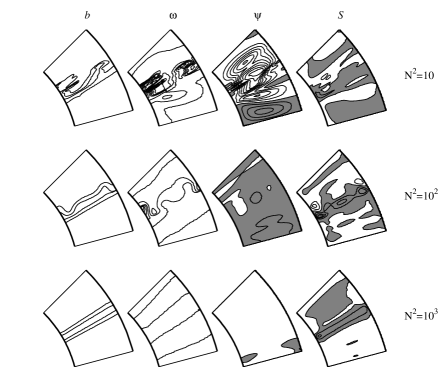
Figure 1.: From left to right, contours of $b$, $\omega$, $\psi$, and $S$, with contour intervals of 0.2, 0.02, $5\times 10^{-5}$, and 0.1, respectively. In the plots for $\psi$ and $S$, grey denotes positive values, white negative ($\psi>0$ corresponds to clockwise circulation). From top to bottom, the three rows are for $N^{2}=10,10^{2},10^{3}$. $A=1$ and time $t=5$ for all three. The range of $r$ is 1 to 1.05, but has been stretched by a factor of 10, and hence looks like 1 to 1.5.

We begin by considering the influence of the stratification. Figure 1 shows results for $N^{2}=10,10^{2},10^{3}$, all for $A=1$ and $f=0$. Within each row, the first panel shows the toroidal field $b$, the second panel the angular velocity $\omega=v/(r\sin\theta)$, the third the meridional circulation $\psi$, and the fourth the entropy $S$. (According to Equation (8), if $a=0$ initially, it will remain zero.) Only the range $\theta\in[45^{o},75^{o}]$ is shown, centered on the flux tube at $\theta=60^{o}$. The radial direction has been stretched by a factor of 10, that is, the actual gap $r\in[1,1.05]$ has been stretched to look like $[1,1.5]$.

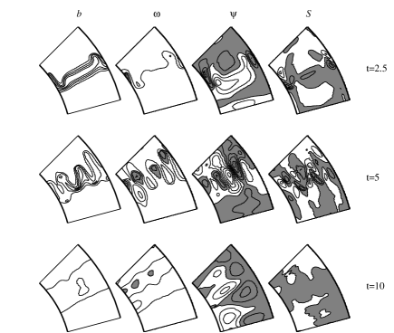
Figure 2.: From left to right, contours of $b$, $\omega$, $\psi$, and $S$, with contour intervals of 0.2, 0.05, $5\times 10^{-5}$, and 1, respectively. In the plots for $\omega$, grey indicates regions where $\omega>1$; for $\psi$ and $S$, grey denotes positive values, as in Figure 1. $N^{2}=10^{3}$, $A=2$, and from top to bottom $t=2.5$, 5, and 10.

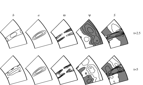
Figure 3.: From left to right, contours of $b$, $a$, $\omega$, $\psi$, and $S$, with contour intervals of 0.2, $10^{-4}$, 0.1, $2\times 10^{-5}$, and 0.2, respectively. In the plots for $\omega$, grey indicates regions where $\omega>1$; for $\psi$ and $S$, grey denotes positive values, as in Figure 1. $N^{2}=10^{3}$, $A=1$, and $f=4\times 10^{-4}$, corresponding to clockwise circulation for the poloidal field. The top row is at $t=2.5$, the bottom row at $t=5$.

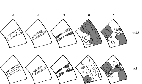
Figure 4.: From left to right, contours of $b$, $a$, $\omega$, $\psi$, and $S$, with contour intervals of 0.2, $10^{-4}$, 0.1, $2\times 10^{-5}$, and 0.2, respectively. $N^{2}=10^{3}$, $A=1$, and $f=-4\times 10^{-4}$, corresponding to counter-clockwise circulation for the poloidal field. (Incidentally, it is perhaps explicitly worth noting that because of the ten-fold stretching in the radial direction, $a_{\theta}$ is actually ten times greater than the spacing of the contour levels might suggest. So in fact $a_{\theta}$ is greater than $a_{r}$.)

Turning to the variation with $N^{2}$, we see that for $N^{2}=10$ the solution has changed significantly from its initial condition, whereas for $N^{2}=10^{3}$ it is almost unchanged. The reason for this is easy to understand: If initially only $b$ and $v$ are non-zero – and if $a$ is always zero – then according to Equations (5) and (7), the only way (apart from the very weak dissipation) for either $b$ or $v$ to change is by inducing a meridional circulation $\psi$. Now, according to Equation (6), the terms $P_{2}(b,b)-P_{2}(v,v)$ will indeed induce such a circulation; these terms are zero only if $\frac{\partial}{\partial z}(b^{2}-v^{2})=0$, which in general is not the case. However, for increasingly strong stratification, the buoyancy term $(r^{-1}\frac{\partial S}{\partial\theta})$ can very effectively suppress the tendency to drive a meridional circulation. That is, having only $b$ and $v$ non-zero is not quite an equilibrium solution to the governing equations, but if $N^{2}$ is sufficiently large, only a very weak circulation $\psi$ will be induced, so according to Equations (5) and (7), $b$ and $v$ will remain almost unchanged. This justifies linear stability analyses such as those of CDG08, where a basic state is simply imposed for $b$ and $v$. In the remainder of this paper we will consider only the strongly stratified case $N^{2}=10^{3}$.

Figure 2 shows the effect of doubling the field strength, to $A=2$. Now even the strong stratification is not enough to stabilize the solution. Instead, we see the development of precisely the radial-shredding instabilities previously studied by CDG08. Here though we follow the full nonlinear evolution, and discover that by $t=10$ the instability has almost completely obliterated the original flux tube.

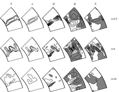
Figure 5.: From left to right, contours of $b$, $a$, $\omega$, $\psi$, and $S$, with contour intervals of 0.2, $5\times 10^{-5}$, 0.1, $5\times 10^{-5}$, and 1, respectively. In the plots for $\omega$, grey indicates regions where $\omega>1$; for $\psi$ and $S$, grey denotes positive values. $N^{2}=10^{3}$, $A=2$, and $f=10^{-4}$. From top to bottom $t=2.5$, 5, and 10.

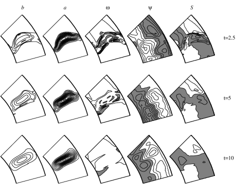
Figure 6.: From left to right, contours of $b$, $a$, $\omega$, $\psi$, and $S$, with contour intervals of 0.2, $5\times 10^{-5}$, 0.1, $5\times 10^{-5}$, and 1, respectively. In the plots for $\omega$, grey indicates regions where $\omega>1$; for $\psi$ and $S$, grey denotes positive values. $N^{2}=10^{3}$, $A=2$, and $f=4\times 10^{-4}$. From top to bottom $t=2.5$, 5, and 10.

3.2 Twisted Flux Tubes

subsec:twist

Figures 3 and 4 show the results for $A=1$ and $f=\pm 4\times 10^{-4}$. That is, the amplitude $A=1$ is as in Figure 1, too low for the shredding instability to occur, and indeed it doesn’t. Nevertheless, the solutions also do not remain virtually stationary, as in the bottom row in Figure 1. Instead, we see the development of highly localized jets in the angular velocity $\omega$. To understand their origin, we return to Equation (5), where the term $P_{1}(b,a)$ is clearly responsible; this term is zero only if contours of $b$ and $a$ coincide, which in general is not the case. Furthermore, because there is no buoyancy force in this equation, no amount of stratification can suppress this effect, very much unlike Figure 1.

Comparing Figures 3 and 4 in detail, we note that reversing the sign of $a$ (that is, the sense of twist in the tube) has exactly the effect one might expect; reversing the sign of $P_{1}(b,a)$ simply reverses the jets. Otherwise the evolution is much the same, and in both cases the flux tubes largely maintain their strength. Note also that jets as concentrated as this would not be detectable by helioseismology, so phenomena such as these could conceivably exist in the real tachocline.

Figure 5 shows results for $A=2$ and $f=10^{-4}$. The toroidal field is therefore as in Figure 2, whereas the poloidal field is half as strong as in Figure 3 (so the nonlinear term $P_{1}(b,a)$ is just as strong as in Figure 3). Initially we see the same jets as in Figures 3 and 4 (and reversing the sign of $f$ again merely reverses the jets). By $t=5$ the evolution is dominated by the same shredding instability as in Figure 2, and the final result is much the same, with the original flux tube largely destroyed. Poloidal fields as weak as this therefore have relatively little influence. However, if we increase the poloidal field strength to $f=4\times 10^{-4}$, it does have a very significant influence, as illustrated in Figure 6. The radial-shredding instability is now completely suppressed, and the flux tube persists up to $t=10$ (and beyond). Note also how the solution has adjusted itself so that contours of $b$ and $a$ do now largely coincide, and correspondingly these localized jets are greatly reduced in strength.

4 Conclusions

sec:conclusion

We have considered the evolution of flux tubes in a thin spherical shell, intended to model solar-type tachoclines. For untwisted tubes we obtain the same radial-shredding instabilities that have previously been studied in the linear regime, and show that in the nonlinear regime these instabilities can very efficiently destroy the original flux tube, simply by shredding it to sufficiently short length-scales for it to dissipate.

For twisted flux tubes, there are a number of possibilities. If the toroidal field is too weak for instabilities to set in, the solution will nevertheless evolve, via the formation of differential-rotation jets, driven directly by the Lorentz forces associated with the twist in the tube. These jets induce a certain amount of structure in the flux tubes, but not enough to disrupt it as the instabilities did.

If the toroidal field is sufficiently strong, and the poloidal field very weak, the shredding instabilities develop much as before, and simply overwhelm the jets driven by the twist. Finally, if the poloidal field is somewhat stronger – but still much weaker than the toroidal – it can suppress the shredding instability. Twisted flux tubes can therefore exist at considerably greater field strengths than untwisted tubes.

Future work will extend this model to 3D and study the interaction of some of the effects presented here with some of the previously known non-axisymmetric magneto-shear instabilities Gilman and Cally (2007).

This work was supported by the UK Science and Technology Facilities Council Grant No. PP/E001092/1. RH’s visit to Australia was supported by a Royal Society International Travel Grant.

References

- Brun and Toomre (2002) Brun, A.S., Toomre, J.: ApJ 570, 865.
- Cally, Dikpati, and Gilman (2008) Cally, P.S., Dikpati, M., Gilman, P.A.: 2008, MNRAS 391, 891. (CDG08)
- Dikpati and Gilman (1999) Dikpati, M., Gilman, P.A.: 1999, ApJ512, 417.
- Dikpati et al. (2009) Dikpati, M., Gilman, P.A., Cally, P.S., Miesch, M.S.: 2009, ApJ 692, 1421.
-
Fan (2004)
Fan, Y.: 2004, Living Rev. Solar Phys. 1,
URL (cited on 1 August 2009):
http://www.livingreviews.org/lrsp-2004-1 - Gilman and Cally (2007) Gilman, P.A., Cally, P.S.: In: Hughes D., Rosner R., Weiss N., eds, 2007, The Solar Tachocline. Cambridge University Press. p 243.
- Gilman and Fox (1997) Gilman, P.A., Fox, P.A.: 1997, ApJ 484, 439.
- Gough and Tayler (1966) Gough, D.O., Tayler, R.J.: 1966, MNRAS 133, 85.
- Hollerbach (2000) Hollerbach, R.: 2000, Int. J. Numer. Meth. Fluids 32, 773.
- Hughes, Rosner, and Weiss (2007) Hughes D., Rosner R., Weiss N., eds, 2007, The Solar Tachocline. Cambridge University Press.
- Watson (1981) Watson, M.: 1981, Geophys. Astrophys. Fluid Dyn. 16, 285.