Epidemic threshold for the SIS model on random networks

Abstract

We derive an analytical expression for the critical infection rate $r_{c}$ of the susceptible-infectious-susceptible (SIS) disease spreading model on random networks. To obtain $r_{c}$, we first calculate the probability of reinfection, $\pi$, defined as the probability of a node to reinfect the node that had earlier infected it. We then derive $r_{c}$ from $\pi$ using percolation theory. We show that $\pi$ is governed by two effects: (i) The requirement from an infecting node to recover prior to its reinfection, which depends on the disease spreading parameters; and (ii) The competition between nodes that simultaneously try to reinfect the same ancestor, which depends on the network topology.

Diseases spread in a population as infected individuals infect other individuals with whom they are in contact. In recent years, several models have been developed to mathematically characterize the spread of diseases Bailey (1975a); Anderson and May (1991); Hethcote (2000). The disease spreading is best modeled as a sparse network, where the individuals are the nodes and the contacts are the links connecting them Moore and Newman (2000); Kuperman and Abramson (2001); Pastor-Satorras and Vespignani (2001a). Two epidemic models of particular importance are the SIR (susceptible/infectious/recovered) Kermack and McKendrick (1927) and SIS (susceptible/infectious/susceptible) Weiss and Dishon (1971); Bailey (1975b); Murray (1993). In these models, the $N$ network nodes are initially susceptible (they currently do not have the disease, but might become infected later), except for one randomly chosen infected node. At each time step, an infected node infects each of its neighbors with probability $r$. Infected nodes remain as such for $\tau$ time steps, after which they become either recovered (cannot further infect or become infected) in SIR or susceptible again in SIS. Hence, in SIS individuals can be infected multiple times.

A fundamental question in the study of epidemics is: will a disease spread throughout the population, or will it die out? The answer to this question depends on the values of the infection and recovery rates, as well as on the nature of the connections between the individuals. For the SIR model on random networks, the epidemic threshold and the critical infection rate above which the disease infects a non-zero fraction of the population were previously derived Pastor-Satorras and Vespignani (2001a); Grassberger (1982); Newman (2002). However, for the SIS model, the calculation of the critical infection rate is significantly more involved due to the possibility of multiple infections of the same node.

Analytical results for SIS on networks exist for a number of specific network models (e.g., a circle, a lattice, a double-layered fully connected network, etc. Liggett (1999); Diekmann et al. (1998); Ball (1999); Neal (2008)). A mean-field analysis of SIS on general random networks has been proposed in Pastor-Satorras and Vespignani (2001b); M. Boguna and Vespignani (2003). In this approach, master equations are written for the number of infected individuals of a given degree. To calculate the epidemic threshold, the mean-field approach assumes that an infected individual has an equal probability to infect each of its neighbors. However, as we show below, the probability of an individual to reinfect the neighbor that had previously infected it (the reinfection probability) is different from the probability to infect the other neighbors.

In this Letter, we derive an analytical expression for the SIS epidemic threshold. We find that the critical infection rate at the threshold is higher than the mean-field approximation for SIS but lower than the critical infection rate for SIR. Simulation results support the accuracy of our expression. To obtain the epidemic threshold, we first calculate the reinfection probability which depends on both the disease spreading parameters and the network topology. Then, using percolation arguments we derive the threshold from the reinfection probability.

To derive the epidemic threshold, some definitions from percolation theory are needed. In a percolation process on a network, links are removed until only a fraction $p$ of the $N$ network nodes remain. This is continued until a critical value, the percolation threshold $p_{c}$, is reached. For $p>p_{c}$, a spanning cluster of order $N$ nodes exists, while for $p<p_{c}$ the network collapses into small clusters Stauffer and Aharony (2004); Bunde and Havlin (1996); Erdős and Rényi (1959); Bollobás (1985); Cohen et al. (2000).

Disease spreading can be seen as a growing percolation process Alexandrowicz (1980), in which, starting from a given seed, links are being added to the growing network with probability $p$. The critical infection rate in which the disease spreads throughout the network is equivalent to the percolation threshold in which a spanning cluster appears. To complete the mapping, we specify the epidemic equivalent of $p$, that is, the probability of a node to infect its neighbor. This probability is different from $r$, since an infected node $i$ (see Fig. 1) can infect its neighbor $j$ only as long as it is still infected, for $\tau$ time steps. Therefore, the desired probability is given by Newman (2002):

$$p=1-(1-r)^{\tau}.$$ (1)

The critical infection rate $r_{c}$ for a given $\tau$ can then be obtained by substituting $p_{c}$ in Eq. (1).

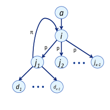
Figure 1: A schematic illustration of the sub-network in which the probabilities of infections are calculated in the text.

To find $p_{c}$, we define $\left\langle n_{i}\right\rangle$, the average number of susceptible nodes infected by an already infected node $i$. If $\left\langle n_{i}\right\rangle>1$, the disease will keep on spreading until a non-zero fraction of the network is covered Madar et al. (2004). In SIR, only the descendants of a node should be taken into account, whereas in SIS, the ancestor could also be reinfected. In terms of Fig. 1, node $i$, once infected, can infect not only its descendants $j_{1},j_{2},...$ (in SIR) but also its ancestor $a$ (in SIS).

The probability of a node that is reached by following a link to have degree $k$ (one incoming link and $k-1$ outgoing links) is $kP(k)/\left\langle k\right\rangle$ where P(k) is the degree distribution of the network nodes. Therefore, as long as the network has a tree like structure and loops are negligible Cohen et al. (2000), the average number of neighbors infected by node $i$ for SIR is given by Madar et al. (2004):

$$\left\langle n_{i}\right\rangle_{\textrm{SIR}}=p\sum_{k}\frac{kP(k)}{\left\langle k\right\rangle}(k-1)\equiv p(\kappa-1),$$ (2)

where $\kappa-1\equiv[\left\langle k^{2}\right\rangle/\left\langle k\right\rangle]-1$ is the branching factor. At the epidemic threshold, $p_{c}(\kappa-1)=1$ Cohen et al. (2000). Writing $p_{c}$ in terms of $r_{c}$ and $\tau$ (Eq. (1)) we obtain:

$$r_{c}=1-\left(\frac{\kappa-2}{\kappa-1}\right)^{1/\tau}.$$ (3)

In SIS, the additional link leading to the ancestor should be incorporated into the calculation. This can be accomplished by making use of an effective branching factor, obtained by replacing $\kappa-1$ by $\kappa$ (the mean field approach). For example, consider node $j_{1}$ in Fig. 1: in addition to the $\kappa-1$ links that are connected to the descendants $d_{1},...,d_{\kappa-1}$, it also has the link to $i$.

However, this approach is too simplistic: the probability of $j_{1}$ to reinfect its ancestor is different from its probability to infect its descendants. This is true since as opposed to the descendants, $i$ is not necessarily susceptible. This is a combined outcome of two effects. First, since $i$ must have been sick before infecting $j_{1}$ in the first place, $j_{1}$ can only reinfect $i$ after $i$ has recovered and became susceptible again (the “time” factor). Moreover, one of the other descendants of $i$ ($j_{2},...,j_{\kappa-1}$ in Fig. 1) might reinfect $i$ before $j_{1}$ does (the “neighbors” factor). Below, we derive an analytical expression for the probability of reinfection $\pi$, taking into account these effects and comparing it to the mean field approach.

Using $\pi$, an expression for $\left\langle n_{i}\right\rangle_{\textrm{SIS}}$ immediately follows:

$$\left\langle n_{i}\right\rangle_{\textrm{SIS}}=p(\kappa-1)+\pi.$$ (4)

The first term is the SIR branching factor (Eq. (2)) and the second is the SIS-specific contribution of the probability to reinfect the ancestor.

Our analysis depends on the assumption that the descendants of an infected node $d_{1},...,d_{\kappa-1}$ are susceptible and therefore the probability to infect them is $p$. This assumption is commonly used in epidemic models when studying disease spreading (e.g., Newman (2002); Pastor-Satorras and Vespignani (2001a)), but limits the validity of the results to the region of at or below the epidemic threshold. For SIR this assumption is trivially true since reinfections are not permitted and the disease spreads directionally down a tree structure. However, for SIS where reinfections are allowed, the disease can spread down and back up the same branch, and thus the neighbors of a just infected node may already be infected. Nevertheless, since at or below the threshold the infection rate is already low, the probability that the disease has spread down and then back up is extremely small Not (a).

To calculate $\pi$ we first obtain the probability $\pi_{t}$ of $j_{1}$ to infect $i$, considering the “time” factor and ignoring the “neighbors” factor. Assume node $i$ has been infected for $s$ time steps before infecting $j_{1}$. Since the total lifetime of the disease is $\tau$ time steps, $i$ remains infected for $(\tau-s)$ time steps after infecting $j_{1}$. Therefore, the total time in which $j_{1}$ is infected and $i$ is not is $\tau-(\tau-s)=s$. The desired probability $\pi_{t}$ is obtained by conditioning on $s$:

$$\pi_{t}=\sum_{s=1}^{\tau}\frac{(1-r)^{s-1}r}{1-(1-r)^{\tau}}[1-(1-r)^{s}]=\frac{1-(1-r)^{\tau+1}}{2-r}$$ (5)

where $(1-r)^{s-1}r/[1-(1-r)^{\tau}]$ is the probability that $i$ infected $j_{1}$ at step $s$ given that $j_{1}$ was eventually infected, and $[1-(1-r)^{s}]$ is the probability that $j_{1}$ infected $i$ in at most $s$ steps.

To complete the derivation of $\pi$, we incorporate the effect of competition (which node is the first to reinfect i) between $j_{1}$ and the other descendants of $i$. Since $i$ is arrived at by following a link from $a$, it will have on average $\kappa-1$ descendants, $j_{1},...,j_{\kappa-1}$. In addition, $i$ can also be reinfected by its ancestor $a$. Therefore Not (b):

$$\pi=\pi_{t}\sum_{k^{\prime}=0}^{\kappa-1}\binom{\kappa-1}{k^{\prime}}\frac{\left(p\pi_{t}\right)^{k^{\prime}}\left(1-p\pi_{t}\right)^{\kappa-1-k^{\prime}}}{k^{\prime}+1}.$$ (6)

To see this, recall that $\pi_{t}$ is the probability of $j_{1}$ to infect $i$, independently of its siblings $a,j_{2},...,j_{\kappa-1}$. Thus, $p\pi_{t}$ is the probability of a sibling of $j_{1}$ to be infected by $i$, and then reinfect $i$. From this, $\pi_{t}\binom{\kappa-1}{k^{\prime}}\left(p\pi_{t}\right)^{k^{\prime}}\left(1-p\pi_{t}\right)^{\kappa-1-k^{\prime}}$ is the probability that exactly $k^{\prime}$ siblings of $j_{1}$, in addition to $j_{1}$ itself, have succeeded to reinfect $i$. However, after the first out of these $k^{\prime}+1$ nodes have reinfected $i$, none of the other $k^{\prime}$ nodes can do so. Since all of these nodes are a-priori equivalent, the probability of $j_{1}$ to successfully reinfect $i$ is obtained by dividing by $k^{\prime}+1$. Finally, the desired probability $\pi$ is obtained by summing over all possible values of $k^{\prime}$.

Next, we compare simulation results for the reinfection probability with the three approximations presented above: (i) $p$ - the reinfection probability assuming it is equal to the probability to infect any other node (mean field approach); (ii) $\pi_{t}$ - the reinfection probability taking into account only the “time” effect (Eq. (5)); (iii) $\pi$ - the reinfection probability according to Eq. (6). Recall that due to the assumption explained above, the equation for $\pi$ is expected to hold only at or below the epidemic threshold. Fig.2 shows that while $\pi_{t}$ is a better estimator of the reinfection probability compared to the mean-field approximation, our Eq. (6) is superior to both and agrees with the simulation results up to the epidemic threshold (indicated with an arrow). For increasing values of $\tau$ (Figs. 2(a) and (c)) two opposing effects occur: While $p$ by itself grows with $\tau$, increasing the probability of reinfection, the growth of $\tau$ also reinforces the “time” and “neighbors” effects, thus attenuating the increase in $\pi$. An increase in $r$ (Figs. 2(b) and (d)) has a similar outcome. As $r$ increases, $p$ increases. In addition, large values of $r$ imply also that $j_{2},...,j_{\kappa-1},a$ are more probable to infect $i$ before $j_{1}$, thus decreasing the total reinfection probability $\pi$.

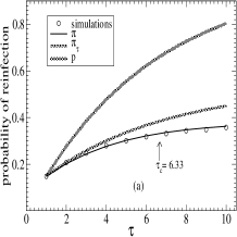
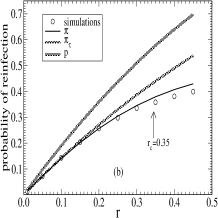
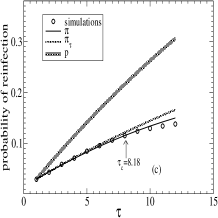
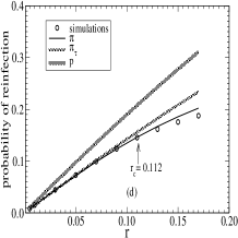
Figure 2: Simulation and theory for the reinfection probability. Three approximations: $p$ (dot-dashed lines),$\pi_{t}$ (dashed lines),$\pi$ (solid lines) are compared with simulation results (see text). Simulation results (circles) were obtained by recording the probability of a infected node to reinfect its ancestors, averaging over many network and disease configurations. The simulations presented are for ER networks but were validated also for SF networks. The epidemic threshold is indicated with an arrow, and is calculated from Eq. (7). (a) $\kappa=2.1$ $r=0.15$ and increasing values of $\tau$. (b) $\kappa=2.1$ $\tau=2$ and increasing values of $r$ (c) $\kappa=5$ and $r=0.03$. (d) $\kappa=5$ and $\tau=2$.

Our analysis has so far been general for all random networks with a prescribed degree distribution $P(k)$. Two specific models are of special interest. The first is the Erdős - Rényi (ER) network model Erdős and Rényi (1959); Bollobás (1985); Erdős and Rényi (1960), in which all links exist with equal probability $\phi$, leading to a Poisson degree distribution $P(k)=e^{-\left\langle k\right\rangle}\left\langle k\right\rangle^{k}/k!$ with average degree $\left\langle k\right\rangle=(N-1)\phi$. The ER network model has become a classic model in random graph theory and was intensively studied in the past few decades. The other model is that of scale free networks (SF) Barabasi and Albert (1999): networks with a broad degree distribution, usually in the form of a power-law, $P(k)\sim k^{-\gamma}$ with $\gamma>2$. It was found that many natural networks are scale-free Barabasi and Albert (1999).

Using our results, the formulation of the critical infection rate for the SIS epidemic model on both ER and SF networks is straightforward. At the threshold,

$$p(r_{c})(\kappa-1)+\pi(r_{c})=1.$$ (7)

For ER networks, $\kappa-1=\left\langle k^{2}\right\rangle/\left\langle k\right\rangle-1=\left\langle k\right\rangle$. Thus, the equation for the critical infection rate is $p(r_{c})\left\langle k\right\rangle+\pi(r_{c})=1$. For SF networks, the value of $\kappa-1$ depends on the degree exponent $\gamma$. Theoretically, $\kappa$ diverges for infinite SF networks with $2<\gamma<3$, leading to the trivial solution $r_{c}=0$. In practice, even for $\gamma<3$ finite networks have finite degrees and thus the epidemic threshold is non-zero Pastor-Satorras and Vespignani (2002).

Simulation results for the critical infection rate $r_{c}$ are presented in Fig. 3, with the theoretical values of $r_{c}$ obtained by numerically solving Eq. (7) for given $\tau$ and $\kappa$. In Fig. 3(a) we plot theory and simulations for $r_{c}$ vs. $\tau$ for ER and SF networks. In Fig. 3(b) we compare our theory, the mean-field approach, and simulation results. For large values of $\tau$, the the mean-field approach deviates by up to 10 percent, while our theory is accurate (see note Not (c)). The inset of Fig. 3(b) compares SIR and SIS.

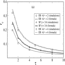
Figure 3: Simulation results for the critical infection rate. (a) Simulation results of $r_{c}$ vs. $\tau$ for ER networks with $\left\langle k\right\rangle=2,4$ and SF networks with $\gamma=3.6$ (symbols), compared to theory (lines) as obtained from Eq. (7). (b) Theoretical values of $r_{c}$ (Eq. (7); solid line) compared to the mean-field approach (obtained by setting $\pi=p$ in Eq. (7); dashed line) and simulation (circles) for $\left\langle k\right\rangle=4$. The inset compares $r_{c}$ (theory and simulations) between SIR (circles) and SIS (squares) with $\left\langle k\right\rangle=2$. Theoretical values (lines) were obtained from Eq. (3) for SIR and from Eq. (7) for SIS. The epidemic threshold was calculated using a method of percolation theory: denote by $S$ the total number of infections; $r_{c}$ was identified as $r$ for which $S\sim N$ Stauffer and Aharony (2004); Bunde and Havlin (1996).

The SIS epidemic model we analyzed has been limited to the case of a fixed recovery time. This is because, to calculate the epidemic threshold, we based our theory on the mapping between bond percolation and the SIR model Newman (2002); Madar et al. (2004). However, it has recently been shown that this mapping is valid only when the recovery time is fixed, whereas variable recovery time introduces correlations not present in the bond percolation model Kenah and Robins (2007). Nevertheless, we argue that our reinfection probability $\pi$ is an upper bound for the reinfection probability with variable recovery time. This can be shown by simulations as well as by the following intuitive argument. Consider the simple case when only the time effect is taken into account and $\pi=\pi_{t}=[1-(1-r)^{(\tau+1)}]/(2-r)$. For a fixed recovery rate, $\tau$ is a random variable, geometrically distributed with mean $\left\langle\tau\right\rangle$. Noting that $\frac{\partial^{2}\pi}{\partial\tau^{2}}\leq 0$ for all $\tau$, it follows from Jensen’s inequality that $\left\langle\pi(\tau)\right\rangle\leq\pi(\left\langle\tau\right\rangle)$.

In summary, we analyzed the propagation of diseases on random networks according to the SIS model. The presence of reinfections in the model poses a great challenge since it can no longer be mapped into a simple branching process. We overcame this problem by calculating the reinfection probability. With this probability, we could recast the problem back into a branching process with an effective branching factor that takes into account not only the descendants of a node, but also its ancestor, weighted by the probability of reinfection. The condition for an outbreak was then found using the reinfection probability and percolation arguments.

We thank the European EPIWORK project and the Israel Science Foundation for financial support and R. Cohen for discussions. S.C. is supported by the Adams Fellowship Program of the Israel Academy of Sciences and Humanities.

References

- Bailey (1975a) N. T. J. Bailey, The Mathematical Theory of Infectious Diseases and its Applications (Hafner Press, New York, 1975a).
- Anderson and May (1991) R. M. Anderson and R. M. May, Infectious Diseases of Humans (Oxford University Press, 1991).
- Hethcote (2000) H. W. Hethcote, SIAM Review 42, 599 653 (2000).
- Moore and Newman (2000) C. Moore and M. E. J. Newman, Phys. Rev. E 61, 5678 5682 (2000).
- Kuperman and Abramson (2001) M. Kuperman and G. Abramson, Phys. Rev. Lett. 86, 2909 2912 (2001).
- Pastor-Satorras and Vespignani (2001a) R. Pastor-Satorras and A. Vespignani, Phys. Rev. Lett. 86, 3200 3203 (2001a).
- Kermack and McKendrick (1927) W. O. Kermack and A. G. McKendrick, Proc. R. Soc. A 115, 700 (1927).
- Weiss and Dishon (1971) G. H. Weiss and M. Dishon, Math Biosic 11, 261 (1971).
- Bailey (1975b) N. T. J. Bailey, The Mathematical Theory of Infectious Diseases (Griffin, London, 1975b).
- Murray (1993) J. D. Murray, Mathematical Biology (Springer-Verlag, 1993).
- Grassberger (1982) P. Grassberger, Math. Biosci. 63, 157 (1982).
- Newman (2002) M. E. J. Newman, Phys. Rev. E 66, 016128 (2002).
- Liggett (1999) T. M. Liggett, Stochastic Interacting systems: contact, voter and exclusion processes (Springer, 1999).
- Diekmann et al. (1998) O. Diekmann, M. C. M. De Jong, and J. A. J. Metz, J. Appl. Prob. 35, 448 (1998).
- Ball (1999) F. Ball, Math. Biosci. 156, 41 (1999).
- Neal (2008) P. J. Neal, J. Appl. Prob. 45, 513 (2008).
- Pastor-Satorras and Vespignani (2001b) R. Pastor-Satorras and A. Vespignani, Phys. Rev. Lett. 86, 3200 (2001b).
- M. Boguna and Vespignani (2003) R. P.-S. M. Boguna and A. Vespignani, Lect. Notes Comput. Sc. 127, 625 (2003).
- Stauffer and Aharony (2004) D. Stauffer and A. Aharony, Introduction to Percolation Theory (Taylor and Francis, 2004), 2nd ed.
- Bunde and Havlin (1996) A. Bunde and S. Havlin, Fractals and Disordered Systems (Springer-Verlag, 1996), 2nd ed.
- Erdős and Rényi (1959) P. Erdős and A. Rényi, Publ. Math. 6, 290 (1959).
- Bollobás (1985) B. Bollobás, Random Graphs (Academic Press, Orlando, 1985).
- Cohen et al. (2000) R. Cohen, K. Erez, D. ben Avraham, and S. Havlin, Phys. Rev. Lett. 85, 4626 (2000).
- Alexandrowicz (1980) Z. Alexandrowicz, Phys. Lett. A 80, 284 (1980).
- Madar et al. (2004) N. Madar, T. Kalisky, R. Cohen, D. Ben-Avraham, and S. Havlin, Eur. Phys. J. B 38 (2), 269 (2004).
- Not (a) To support the argument that at or below the threshold the descendants of an infected node are susceptible, we directly measured, by computer simulations the probability that a neighbor of an infected node is susceptible and the results show that at or below the epidemic threshold, this probability is indeed very close to 1.
- Not (b) More accurately, one needs to distinguish between and since had originally infected and is thus expected to be infected with higher probability. However, simulations show that the change in due to this effect is negligible.
- Erdős and Rényi (1960) P. Erdős and A. Rényi, A. Publ. Math. Inst. Hung. Acad. Sci. 5, 1760 (1960).
- Barabasi and Albert (1999) A.-L. Barabasi and R. Albert, Science 286, 509 (1999).
- Pastor-Satorras and Vespignani (2002) R. Pastor-Satorras and A. Vespignani, Phys. Rev. E 65, 035108 (2002).
- Not (c) The difference between our theory and the MF approach is nicely demonstrated using the percolation threshold, . For the MF approach , and thus for a given , is independent of , while according to our theory depends on . For the parameters used in Fig.3(b), the MF approach yields for any while for our theory approaches for large .
- Kenah and Robins (2007) E. Kenah and J. M. Robins, Phys. Rev. E 036113, 76 (2007).