Effect of pseudogap formation on the penetration depth of underdoped high $T_{c}$ cuprates

Abstract

The penetration depth is calculated over the entire doping range of the cuprate phase diagram with emphasis on the underdoped regime. Pseudogap formation on approaching the Mott transition, for doping below a quantum critical point, is described within a model based on the resonating valence bond spin liquid which provides an ansatz for the coherent piece of the Green’s function. Fermi surface reconstruction, which is an essential element of the model, has a strong effect on the superfluid density at $T=0$ producing a sharp drop in magnitude, but does not change the slope of the linear low temperature variation. Comparison with recent data on Bi-based cuprates provides validation of the theory and shows that the effects of correlations, captured by Gutzwiller factors, are essential for a qualitative understanding of the data. We find that the Ferrell-Glover-Tinkham sum rule still holds and we compare our results with those for the Fermi arc and the nodal liquid models.

I Introduction

The initial discovery of superconductivity in the cuprates precipitated a rush to find higher values of the critical temperature $T_{c}$. In this onslaught, not only were new superconducting members of the cuprate family discovered but it was quickly realized that, through oxygen doping or doping with other elements, a particular compound could display a range of $T_{c}$ values. With hole-doping, in particular, these $T_{c}$ values could be quite high and showed a dome for $T_{c}$ as a function of doping in the phase diagram. While studying optimal doping for the maximum $T_{c}$ became the primary focus in initial research, it was later appreciated that the unusual phase diagram of these materials was of great interest in itself. Understanding why a maximum $T_{c}$ exists and what controls the reduction of $T_{c}$ away from maximum is hoped to elucidate the physics of the interactions involved. Ideally this would give direction for what might be attempted in materials development in order to enhance $T_{c}$.

Further research into the general phase diagram occurred on many fronts, with evidence of an antiferromagnetic (AFM) insulating state in the parent compound and at low doping, and strange metallic behavior in the normal state above the superconducting dome. The most intriguing discovery is possibly the presence of what is now termed a “pseudogap” feature, occurring in the normal state on the underdoped side of the superconducting dome, which exists for higher temperatures as the AFM state is approached.timusk This pseudogap is an energy gap-like feature seen in normal state properties which has led to a number of imaginative theoretical proposals for its existence. Superconductivity in the cuprates is now thought to have $d$-wave superconducting pairing, most likely due to spin-fluctuations.carbottenature ; inversion It is thought, therefore, that the approach towards the AFM state should enhance the spin-fluctuation pairing interaction $V$ and hence increase $T_{c}$. However, if this pseudogap represents a competing phase, possibly associated with the AFM-Mott insulator, it could be responsible for a reduction in the electronic density of states at the Fermi level $N(0)$ which could then reduce the superconducting $T_{c}$ which depends on $N(0)V$ in simple BCS theory. Consequently, it is natural that many proposals for the pseudogap state have been based on a competing phase, such as, the $d$-density wave theory.laughlin Others have been suggested which include the ideas of preformed pairsemery ; randeria ; alvarez ; levin arising above $T_{c}$.

The pseudogap phase and how it may affect superconductivity has become a major focus of both theoretical and experimental work. Even knowledge of where the pseudogap line in the phase diagram might end [possibly at $T=0$ and possibly as a quantum critical point (QCP)] is still a matter of debate. Some experiments suggest it ends on the edge of the superconducting dome on the overdoped side and others place it ending at $T=0$ inside the superconducting zone anywhere from optimal doping to overdoped.hufner It should be noted that other works on QCPs in heavy fermion superconductors usually suggest such a point existing under the superconducting dome.HF

In spite of mounting experimental work on the underdoped cuprate superconductors, it has been hard to develop a microscopic theory that can build in the physics associated with the approach from the metallic state to the Mott insulator and give a workable formalism, which includes doping, for providing theoretical insights and predictions for experiments both in the normal and superconducting state (including the idea of a pseudogap). Further to this issue has been the more recent experimental development where a possible reconstruction of the Fermi surface in the underdoped cuprates has been found to occur based on seeing Fermi pockets from de Haas-van Alphen experimentslouis and or Fermi arcs in angle-resolved photoemission (ARPES) experiments.arpesarcs There has also been one report of an observation of pockets from ARPES.zhou Moreover, there has been indirect evidence of arcs from other experiments, such as optical spectroscopyhwang , specific heatstorey and scanning tunneling spectroscopydavis measurements. Indeed, attempting to resolve the arc versus pocket debate has been the subject of numerous papers.

One theory which is promising in this regard has been due to Yang, Rice and Zhangyrz (YRZ) which is based on previous studies of a resonating valence bond (RVB) spin liquid state originally proposed by Andersonanderson . The merit of the YRZ approach is that they have used previous numerical and theoretical RVB-type studies to develop an ansatz for the many-body Green’s function that would represent the RVB spin liquid. This ansatz builds in the approach to the AFM-Mott insulator and shows a reconstructed Fermi surface which is a large Fermi surface when there is no pseudogap, above optimal doping, but is reconstructed to small Fermi or Luttinger pockets (which look more like arcs when the quasiparticle weight is included) for the underdoped case. The pseudogap opens up around the AFM Brillouin zone in this theory and it gaps out or reconstructs part of the Fermi surface. So far this theory has been used to evaluate a number of experimental propertiesbelen ; emilia ; yrzarpes ; james with good qualitative agreement and, in the same spirit as BCS theory, using this ansatz allows us to determine what are the essential elements that should go into a more sophisticated microscopic theory should it be developed in the future.

In this work, we wish to examine the long-standing puzzle associated with the penetration depth measurements. The penetration depth was one of the first experiments to clearly indicate that a $d$-wave order parameter symmetry for the superconductivity was present in the cuprates.bonnhardy This was an extremely important result in influencing the direction of research in this field as it allowed for the elimination of a number of possible mechanisms for Cooper pairing. It also clarified the need for very high quality samples to remove the obscuring features due to impurities. The essential observation from the experiment was that the superfluid density $\rho_{s}(T)$, which is related to the penetration depth $\lambda(T)$ by $\rho_{s}(T)\propto 1/\lambda^{2}(T)$, showed a low temperature linear $T$ behavior as expected for a clean BCS $d$-wave superconductor, i.e., $\rho_{s}(T)=\rho_{s}(0)-bT$. However, in the underdoped regime, it is knownuemura ; leeandwen ; franz that while the zero temperature value of the superfluid density depends strongly on the doping $x$, the coefficient $b$ of the first linear-in-$T$ correction is much less sensitive to $x$. This result cannot be understood within a simple BCS $d$-wave model. Our goal in this paper is to study the penetration depth in the YRZ model and to see if the experimental data, with its doping dependence, can be explained by this theory. Furthermore, we wish to see if there is evidence for a reconstructed Fermi surface in the penetration depth data. With this study we can develop a better understanding of the physics which is giving rise to this non-BCS behavior of the doping dependence of the penetration depth.

Our paper is structured as follows. In Section II, we introduce the basic features of the YRZ theory that enter into our calculations. This is followed by a discussion of the penetration depth formula used in this work and its various limits, given in Section III. In Section IV, we summarize some theoretical formulas associated with the frequency-dependent optical conductivity, a quantity which is also related to the penetration depth. This will aid in our discussion of the Drude weight and the sum rule. We then present our results in Section V and provide our conclusions in Section VI.

II Theoretical model of YRZ

The YRZ model provides an ansatz for the coherent part of the many-body Green’s function for the case of a doped RVB spin liquid. It includes a dependence on doping $x$ and is given as:yrz ; yrzarpes

$$G(\bm{k},\omega,x)=\sum_{\alpha=\pm}\frac{g_{t}W^{\alpha}_{\bm{k}}}{\omega-E^{\alpha}_{\bm{k}}-\Delta_{\rm sc}^{2}/(\omega+E^{\alpha}_{\bm{k}})},$$ (1)

where

$$E_{\bm{k}}^{\pm} = \frac{{\xi_{\bm{k}}-\xi_{\bm{k}}^{0}}}{2}\pm E_{\bm{k}},$$

$$E_{\bm{k}} = \sqrt{\tilde{\xi_{\bm{k}}}^{2}+\Delta_{\rm pg}^{2}},$$

$$\tilde{\xi_{\bm{k}}} = \frac{(\xi_{\bm{k}}+\xi_{\bm{k}}^{0})}{2},$$

$$W_{\bm{k}}^{\pm} = \frac{1}{2}\left({1\pm\frac{{\tilde{\xi_{\bm{k}}}}}{E_{\bm{k}}}}\right).$$ (2)

In these expressions $\xi_{\bm{k}}^{0}=-2t(x)(\cos k_{x}a+\cos k_{y}a)$ is the first nearest neighbor tight-binding dispersion, which introduces the antiferromagnetic Brillouin zone boundary (AFBZ) into the Green’s function along which the pseudogap $\Delta_{\rm pg}$ develops. The band structure $\xi_{\bm{k}}=-2t(x)(\cos k_{x}a+\cos k_{y}a)-4t^{\prime}(x)\cos k_{x}a\cos k_{y}a-2t^{\prime\prime}(x)(\cos 2k_{x}a+\cos 2k_{y}a)-\mu_{p}$ is taken from tight-binding for a system which includes hopping terms up to third nearest neighbor, with $\mu_{p}$, a chemical potential determined by the Luttinger sum rule.yrz Doping dependence enters in three ways into the Green’s function. First, the band structure is doping dependent through the hopping coefficients: $t(x)=g_{t}(x)t_{0}+3g_{s}(x)J\chi/8$, $t^{\prime}(x)=g_{t}(x)t_{0}^{\prime}$, and $t^{\prime\prime}(x)=g_{t}(x)t_{0}^{\prime\prime}$, where $g_{t}(x)=2x/\left(1+x\right)$ and $g_{s}(x)=4/(1+x)^{2}$ are the Gutzwiller factors and $J/t_{0}=1/3$ and $\chi=0.338$. YRZ use $t^{\prime}_{0}/t_{0}=-0.3$, $t^{\prime\prime}_{0}/t_{0}=0.2$, a choice of parameters to match this energy dispersion to that calculated for Ca₂CuO₂Cl₂ (Ref. yrz ). The $x$-dependence of these coefficients reflects the fact that strong correlations will narrow the bands as the Mott insulator is approached. Second, the coherent part of the Green’s function changes with doping with a Gutzwiller factor given by $g_{t}\equiv g_{t}(x)$. Such factors reflect the projection out of doubly occupied states and the approach to the atomic limit. Third, the magnitude of the pseudogap, $\Delta_{\rm pg}$, and superconducting gap, $\Delta_{\rm sc}$, are also doping dependent, as inferred from experiment and the behavior of $T_{c}$. These gaps are taken to be $d$-wave, such that we can write them as $\Delta_{\rm pg}=\frac{\Delta_{\rm pg}^{0}(x)}{2}(\cos k_{x}a-\cos k_{y}a)$ and $\Delta_{\rm sc}=\frac{\Delta_{\rm sc}^{0}(x)}{2}(\cos k_{x}a-\cos k_{y}a)$, respectively, with $a$ the lattice constant, $\Delta^{0}_{\rm pg}(x)/t_{0}=0.6(1-x/0.2)$ and $\Delta^{0}_{\rm sc}(x)/t_{0}=0.14(1-82.6(x-0.2)^{2})$. In general, the gap could contain many higher harmonicsbranch1995 as is also the case in conventional superconductorstomlinson ; leung1 ; leung2 but such complications are not essential for a first understanding. From Eq. (1), one can extract the YRZ spectral function $A(\bm{k},\omega)$ and see that there are four energy branches, given by the energies, $\pm E_{S}^{\alpha}$, where $E^{\alpha}_{S}=\sqrt{(E_{\bm{k}}^{\alpha})^{2}+\Delta_{\rm sc}^{2}}$. Following the usual development of the equations of superconductivity, both the regular and anomalous spectral functions are found to be:

$$A(\bm{k},\omega) = \sum_{\alpha=\pm}g_{t}W_{\bm{k}}^{\alpha}[(u^{\alpha})^{2}\delta(\omega-E^{\alpha}_{S})+(v^{\alpha})^{2}\delta(\omega+E^{\alpha}_{S})],$$

$$B(\bm{k},\omega) = \sum_{\alpha=\pm}g_{t}W_{\bm{k}}^{\alpha}u^{\alpha}v^{\alpha}[\delta(\omega-E^{\alpha}_{S})-\delta(\omega+E^{\alpha}_{S})],$$ (4)

where

$$u^{\alpha} = \biggl{[}\frac{1}{2}\biggl{(}1+\frac{E_{\bm{k}}^{\alpha}}{E^{\alpha}_{S}}\biggr{)}\biggr{]}^{1/2},$$ (5)

$$v^{\alpha} = \biggl{[}\frac{1}{2}\biggl{(}1-\frac{E_{\bm{k}}^{\alpha}}{E^{\alpha}_{S}}\biggr{)}\biggr{]}^{1/2}.$$ (6)

These two spectral functions enter the expressions for the penetration depth and the optical conductivity which are described in the following sections. In the limit of $\Delta_{\rm sc}=0$ but with a finite pseudogap, there are still two branches in the quasiparticle energy dispersion as shown in Fig. 1(b) for various symmetry directions in the first quadrant of the square Brillouin zone. The weighting factors $W_{\bm{k}}^{\alpha}$ are shown as upright bars of varying height in the third dimension. Comparing with a case for no pseudogap where there is just the one energy dispersion with full weight [Fig. 1(a)], we see that a gap in energy due to the pseudogap formation has opened around the antinodal direction in the Brillouin zone quadrant at $(\pi,0)$ and $(0,\pi)$, and along the AFBZ from $(\pi,0)$ to $(0,\pi)$. The presence of the two bands gives rise to interband transitions in the frequency-dependent optical conductivity and a depletion of the intraband Drude component as we will later discuss.

In the following work, we will also examine several other models in relation to the YRZ model. We will refer to a Fermi liquid which is just the case of taking the pseudogap to be zero in our formalism. We also use the term YRZ modified (YRZ mod.). In the YRZ model, the presence of the pseudogap reconstructs the large Fermi surface (found on the overdoped side of the phase diagram) into a small Fermi pocket. If we use the YRZ model but take the superconducting $d$-wave gap to be finite only in the region of the Fermi pocket and to be zero beyond the pocket towards the antinodal direction, then we will call this YRZ modified. In conventional superconductorstomlinson ; leung1 ; leung2 such as Pb and Al, there are directions where the Fermi surface is gapped out by the crystal potential and one finds that the superconducting gap is also zero there. In the present case it is the pseudogap which prevents the superconducting gap from having its full amplitude in certain regions.

Two other models in the literature are the nodal liquid and the Fermi arc model. In these two models, the pseudogap is taken to be on the large Fermi surface given by $\xi_{\bm{k}}$. In the nodal liquid, both the pseudogap and superconducting gaps are active over the entire Fermi surface. In the arc model, the pseudogap is only finite in a region of the Fermi surface near that antinodal direction on an arc of the large Fermi surface that is defined by a critical angle $\theta_{c}$ measured at the $(\pi,\pi)$ point from the Brillouin zone boundary towards the nodal direction.james

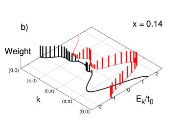
Figure 1: (Color online) The electronic band structure for (a) $x=0.2$ with no pseudogap and for (b) $x=0.14$ with a pseudogap. In the YRZ model for the pseudogapped normal state, two bands, $E_{\bm{k}}^{+}$ and $E_{\bm{k}}^{-}$, exist with ${\bm{k}}$-dependent weighting factors $W_{\bm{k}}^{+}$ and $W_{\bm{k}}^{-}$, respectively, shown as a peak of height set by the weight. The $E_{\bm{k}}^{-}$ band is the lower energy band shown in heavy black and the $E_{\bm{k}}^{+}$ band is the higher energy band shown in lighter red.

III Penetration Depth

The London penetration depth $\lambda(T)$ is given by the zero frequency limit of the imaginary part of the optical conductivity $\sigma(T,\Omega)$ at temperature $T$. Specifically,

$$\frac{1}{\lambda^{2}(T)}=\displaystyle\lim_{\Omega\to 0}\frac{4\pi}{c^{2}}\Omega\rm{Im}\sigma(T,\Omega),$$ (7)

where $c$ is the velocity of light. The imaginary part of $\sigma(T,\Omega)$ has both a contribution from the paramagnetic and diamagnetic part of the current. A particularly transparent formal expression, which manifestly vanishes when the superconducting gap vanishes, results when both contributions are treated on the same footingbranch ; radtke

$$\frac{1}{\lambda^{2}(T)}=\displaystyle\lim_{\Omega\to 0}\frac{16\pi e^{2}}{c^{2}}\sum_{\bm{k}}v_{k_{x}}^{2}$$

$$\times \int d\omega^{\prime}d\omega^{\prime\prime}\lim_{\bm{q}\to 0}\biggl{(}\frac{f(\omega^{\prime\prime})-f(\omega^{\prime})}{\omega^{\prime\prime}-\omega^{\prime}}\biggr{)}B(\bm{k}+\bm{q},\omega^{\prime})B(\bm{k},\omega^{\prime\prime}),$$

where $e$ is the electron charge and $f(\omega)$ is the Fermi function $1/[1+\exp(\beta\omega)]$, with $\beta=1/(k_{B}T)$ and $k_{B}$ the Boltzmann constant. $B({\bm{k}},\omega)$ is the anomalous spectral density previously introduced and is proportional to the superconducting gap. Consequently, this expression vanishes in the normal state as it must. After some lengthy but straightforward algebra, one arrives at a more explicit formula for $1/\lambda^{2}(T)$ in the YRZ model of the form

$$\frac{1}{\lambda^{2}(T)} = \frac{16\pi e^{2}}{c^{2}}\sum_{\bm{k}}v_{k_{x}}^{2}$$ (9)

$$\times \biggl{[}(W_{\bm{k}}^{+})^{2}(u^{+}v^{+})^{2}\biggl{(}2\frac{\partial f(E^{+}_{S})}{\partial E^{+}_{S}}+\frac{1-2f(E_{S}^{+})}{E_{S}^{+}}\biggr{)}$$

$$+ (W_{\bm{k}}^{-})^{2}(u^{-}v^{-})^{2}\biggl{(}2\frac{\partial f(E^{-}_{S})}{\partial E^{-}_{S}}+\frac{1-2f(E_{S}^{-})}{E_{S}^{-}}\biggr{)}$$

$$+ 4W_{\bm{k}}^{+}W_{\bm{k}}^{-}u^{+}v^{+}u^{-}v^{-}\biggl{(}\frac{f(E_{S}^{+})-f(E_{S}^{-})}{E_{S}^{+}-E_{S}^{-}}$$

$$\qquad+\frac{1-f(E_{S}^{+})-f(E_{S}^{-})}{E_{S}^{+}+E_{S}^{-}}\biggr{)}\biggr{]}.$$

This formula is for the clean limit and ignores the inelastic effects which are not large for the penetration depth.ewald Only the coherent part of the Green’s function contributes to the condensate. Note that we have suppressed for now the factor of $g_{t}^{2}$ which weights this quantity in the YRZ model. We will be presenting all of our numerical work for $1/\lambda^{2}(T)$ in units of $e^{2}t_{0}/\hbar^{2}d$, where $d$ is the $c$-axis distance per Cu-O plane (not shown explicitly in the superfluid density formulas given here which are written for 2 dimensions).

Our basic formula, Eq. (9), can be reduced in simpler models such as the nodal liquid or the usual Fermi arc model. In both cases, the pseudogap is placed on the Fermi surface. For the arc model it is nonzero only on arcs about the antinodal direction. To place the pseudogap on the Fermi surface instead of having it on the antiferromagnetic Brillouin zone, we take $\xi_{\bm{k}}^{0}$ to be equal to $\xi_{\bm{k}}$ so that $E_{\bm{k}}^{\pm}=\pm E_{\bm{k}}$, and $W_{\bm{k}}^{\pm}=(1\pm\xi_{\bm{k}}/E_{\bm{k}})/2$, with $E_{\bm{k}}=\sqrt{\xi_{\bm{k}}^{2}+\Delta_{\rm pg}^{2}}$. It follows that $E_{S}^{\pm}=\sqrt{\xi_{\bm{k}}^{2}+\Delta_{\rm pg}^{2}+\Delta_{\rm sc}^{2}}\equiv E_{S}$, $W_{\bm{k}}^{+}+W_{\bm{k}}^{-}=1$, $(u^{\pm})^{2}=(1+E_{\bm{k}}/E_{S})/2\equiv u^{2}$, $(v^{\pm})^{2}=(1-E_{\bm{k}}/E_{S})/2\equiv v^{2}$, and $u^{\pm}v^{\pm}=uv=\Delta_{\rm sc}/2E_{S}$. We then obtain

$$\frac{1}{\lambda^{2}(T)} = \frac{16\pi e^{2}}{c^{2}}\sum_{\bm{k}}v_{k_{x}}^{2}(uv)^{2}\biggl{(}2\frac{\partial f(E_{S})}{\partial E_{S}}+\frac{1-2f(E_{S})}{E_{S}}\biggr{)}$$

$$= \frac{4\pi e^{2}}{c^{2}}\sum_{\bm{k}}v_{k_{x}}^{2}\frac{\Delta_{\rm sc}^{2}}{E_{S}^{2}}\biggl{\{}-\frac{\partial}{\partial E_{S}}+\frac{1}{E_{S}}\biggr{\}}{\rm tanh}\biggl{(}\frac{\beta E_{S}}{2}\biggr{)}.$$

If we further take the pseudogap to be zero $E_{S}=\sqrt{\xi_{\bm{k}}^{2}+\Delta_{\rm sc}^{2}}$ then Eq. (LABEL:eq:bpen) becomes a well-known formula for the Fermi liquid (FL) penetration depth in BCS theory.donovan1 ; donovan2 ; donovan3 ; franz ; misawa With the pseudogap non-zero, we will refer to Eq. (LABEL:eq:bpen) as the nodal liquid limit and if the pseudogap is cut off at a certain critical angle $\theta_{c}$ away from the antinodal direction so that there is no pseudogap on an arc about the nodal direction, we will refer to this as the arc model.

Examining various limits of Eq. (LABEL:eq:bpen) provides understanding of the physics when a pseudogap is present. We recall that for the BCS case with no pseudogap, at zero temperature the tanh$(\beta E/2)$ is equal to 1 and the $T=0$ limit of the penetration depth takes on a particularly simple form

$$\frac{1}{\lambda^{2}(0)} = \frac{2\pi e^{2}}{c^{2}}N(0)v_{F}^{2}$$

$$\times \int_{0}^{2\pi}\frac{d\theta}{2\pi}\int_{-\infty}^{+\infty}d\epsilon\frac{[\Delta^{0}_{\rm sc}\cos(2\theta)]^{2}}{\{\epsilon^{2}+[\Delta^{0}_{\rm sc}\cos(2\theta)]^{2}\}^{3/2}},$$

where the continuum limit of the free electron bands has been taken to simplify the mathematics and $N(0)$ is the electronic density of states, assumed to be constant. The ratio of the electron density to the electron mass $n/m=N(0)v_{F}^{2}$. Further, the last integral over energy in Eq. (LABEL:eq:pencont) is independent of the factor of $[\Delta_{\rm sc}^{0}\cos(2\theta)]$ and equal to 2. The angular integration normalized to $2\pi$ is then trivially equal to 1. Thus we obtain the well-known result that $1/\lambda^{2}(0)=4\pi ne^{2}/mc^{2}$. Moreover, in the limit $T\to 0$, the leading temperature dependence is given by the derivative term $(-\partial/\partial E)$ in Eq. (LABEL:eq:bpen). If we write for simplicity $\Delta_{S}\equiv\Delta^{0}_{\rm sc}\cos(2\theta)$, we arrive at

$$\frac{\lambda^{2}(0)}{\lambda^{2}(T)}=1-\beta\int_{0}^{2\pi}\frac{d\theta}{2\pi}\int_{-\infty}^{+\infty}d\epsilon\frac{\Delta^{2}_{S}}{\epsilon^{2}+\Delta^{2}_{S}}\frac{e^{\beta\sqrt{\epsilon^{2}+\Delta^{2}_{S}}}}{[e^{\beta\sqrt{\epsilon^{2}+\Delta^{2}_{S}}}+1]^{2}}.$$ (12)

As $T\to 0$ this last integral is strongly peaked about $\epsilon\sim 0$ and $\Delta_{S}\sim 0$ (i.e., the nodal direction) and we obtain the standard result

$$\frac{1}{\lambda^{2}(T)}=\frac{4\pi ne^{2}}{mc^{2}}\biggl{[}1-2\ln 2\frac{k_{B}T}{\Delta^{0}_{\rm sc}}\biggr{]}.$$ (13)

For the case of the nodal liquid, the pseudogap is assumed to go like $\Delta_{\rm pg}(\theta)=\Delta^{0}_{\rm pg}\cos(2\theta)$ over the entire Fermi surface as does the superconducting gap. In this case, expression (LABEL:eq:bpen) can be cast in the form of the standard BCS case with two changes. The square of the gap amplitude is to be replaced by the sum of the squares of superconducting and pseudogap, i.e., $\Delta_{\rm sc}^{0}\to\sqrt{(\Delta_{\rm sc}^{0})^{2}+(\Delta_{\rm pg}^{0})^{2}}$, and an overall factor of $(\Delta_{\rm sc}^{0})^{2}/[(\Delta_{\rm sc}^{0})^{2}+(\Delta_{\rm pg}^{0})^{2}]$ now multiplies the entire expression. This leads immediately to the result

$$\frac{1}{\lambda^{2}(T)} = \frac{4\pi ne^{2}}{mc^{2}}\frac{(\Delta^{0}_{\rm sc})^{2}}{(\Delta_{\rm sc}^{0})^{2}+(\Delta_{\rm pg}^{0})^{2}}$$ (14)

$$\times \biggl{[}1-2\ln 2\frac{k_{B}T}{\sqrt{(\Delta_{\rm sc}^{0})^{2}+(\Delta_{\rm pg}^{0})^{2}}}\biggr{]}.$$

In this case the London penetration depth at $T=0$ is no longer simply a normal state property but depends explicitly on the value of the superconducting gap amplitude. Also, the normalized slope of the linear-in-temperature term is greatly reduced when the pseudogap is large. While this limit is helpful because of its simplicity, we will see that it does not describe the YRZ results well. By contrast, the arc model which is closely related to the above equations does well in capturing the main physics contained in the more mathematically complex YRZ model. Before turning to this case, we note that at $T=0$, when the pseudogap is small compared with the superconducting gap, the penetration depth is modified to $1/\lambda^{2}(0)=(4\pi ne^{2}/mc^{2})[1-(\Delta^{0}_{\rm pg}/\Delta^{0}_{\rm sc})^{2}]$ which tells us that the superfluid density is effectively reduced over its no pseudogap value. The pseudogap competes with the superconductivity for phase space.

Introduction of an arc over which the pseudogap is zero, while finite from antinodal direction to $\theta_{c}$, modifies Eq. (LABEL:eq:pencont) but at the same time leaves the second integral in Eq. (12) completely unaltered because, for sufficiently small temperature, only the angular region very close to the nodal direction is of importance. But in these regions, the pseudogap is zero so that the first derivative term $-\partial/\partial E$ in Eq. (LABEL:eq:bpen) is unaffected by the pseudogap. Therefore, we obtain for this term $(4\pi ne^{2}/mc^{2})[-(2\ln 2)k_{B}T/\Delta^{0}_{\rm sc}]$ which is completely unchanged from its Fermi liquid value. This is not so for the value of the zero temperature penetration depth. This quantity does know about the pseudogap. In the continuum approximation, it is given by

$$\frac{1}{\lambda^{2}(0)}=\frac{2\pi ne^{2}}{mc^{2}}$$

$$\times \int_{0}^{2\pi}\frac{d\theta}{2\pi}\int_{-\infty}^{+\infty}d\epsilon\frac{[\Delta^{0}_{\rm sc}\cos(2\theta)]^{2}}{\{\epsilon^{2}+[(\Delta^{0}_{\rm sc})^{2}+(\bar{\Delta}^{0}_{\rm pg})^{2}]\cos^{2}(2\theta)\}^{3/2}},$$

where for simplicity we have assumed the pseudogap to have the same angular dependence as the superconducting gap, namely the $d$-wave $\cos(2\theta)$ dependence. Here the bar on $\bar{\Delta}^{0}_{\rm pg}$ is to mean that it is zero in the interval $\theta_{c}$ to $\pi/4$ and all other symmetry related intervals. Next we note that the energy integral will give $2(\Delta^{0}_{\rm sc})^{2}/[(\Delta_{\rm sc}^{0})^{2}+(\Delta_{\rm pg}^{0})^{2}]$ from the regions where $\bar{\Delta}_{\rm pg}^{0}$ is nonzero (antinodal) and 2 from the regions where $\bar{\Delta}_{\rm pg}^{0}$ is zero (nodal). We finally get

$$\frac{1}{\lambda^{2}(0)}=\frac{4\pi ne^{2}}{mc^{2}}\biggl{[}1-\frac{4\theta_{c}}{\pi}\frac{(\Delta^{0}_{\rm pg})^{2}}{(\Delta_{\rm sc}^{0})^{2}+(\Delta_{\rm pg}^{0})^{2}}\biggr{]}.$$ (16)

For $\theta_{c}=0$ (that is, no pseudogap), we get back the classical London result of Eq. (LABEL:eq:pencont) after integration over energy and angle. For $\theta_{c}=\pi/4$, the nodal liquid result of Eq. (14) in the $T\to 0$ limit is obtained. When the pseudogap $\Delta_{\rm pg}^{0}=0$, we recover the known result of Fermi liquid theory, that the zero temperature value of the penetration depth depends only on normal state parameters and not on the explicit value of the superconducting gap itself. When the pseudogap is small as compared to the superconducting gap, the correction to 1 in Eq. (16) is small and of order $(4\theta_{c}/\pi)(\Delta_{\rm pg}^{0}/\Delta_{\rm sc}^{0})^{2}$. In the opposite limit of large pseudogap, the superconducting gap drops out and the correction is $4\theta_{c}/\pi$, explicitly independent of both gaps. The pseudogap, however, implicitly determines the critical angle $\theta_{c}$ related to the part of the Fermi surface over which the pseudogap is non-zero.

IV Optical Conductivity

The real part of the optical conductivity, ${\rm Re}\sigma(T,\Omega)$, is given byemilia

$${\rm Re}\sigma(T,\Omega)=\frac{2\pi e^{2}}{\Omega}\sum_{\bm{k}}v_{k_{x}}^{2}\int_{-\infty}^{+\infty}d\omega[f(\omega)-f(\omega+\Omega)][A({\bm{k}},\omega)A({\bm{k}},\omega+\Omega)+B({\bm{k}},\omega)B({\bm{k}},\omega+\Omega)].$$ (17)

In the clean limit of the YRZ model, we obtain, after long but straightforward algebra, the expression

$${\rm Re}\sigma(T,\Omega) = 2\pi e^{2}\sum_{\bm{k}}v_{k_{x}}^{2}\biggl{\{}\delta(\Omega)\biggl{[}-\frac{\partial f(E^{+}_{S})}{\partial E^{+}_{S}}(W_{\bm{k}}^{+})^{2}-\frac{\partial f(E^{-}_{S})}{\partial E^{-}_{S}}(W_{\bm{k}}^{-})^{2}\biggr{]}$$

$$+ W_{\bm{k}}^{+}W_{\bm{k}}^{-}\biggl{[}(u^{-}v^{+}-u^{+}v^{-})^{2}\frac{1-f(E_{S}^{+})-f(E_{S}^{-})}{E_{S}^{+}+E_{S}^{-}}\delta(\Omega-E_{S}^{+}-E_{S}^{-})$$

$$- (u^{+}u^{-}+v^{+}v^{-})^{2}\frac{f(E_{S}^{+})-f(E_{S}^{-})}{E_{S}^{+}-E_{S}^{-}}[\delta(\Omega-E_{S}^{+}+E_{S}^{-})+\delta(\Omega+E_{S}^{+}-E_{S}^{-})]\biggr{]}\biggr{\}}.$$

The first term in Eq. (LABEL:eq:cond2) is proportional to $\delta(\Omega)$ and a Drude weight can be defined as

$$\frac{W_{D}}{2} \equiv \int_{0}^{\infty}{\rm Re}\sigma_{\rm Drude}(T,\Omega)d\Omega$$ (19)

$$= 2\pi e^{2}\sum_{{\bm{k}},\alpha=\pm}v_{k_{x}}^{2}\biggl{[}-\frac{\partial f(E^{\alpha}_{S})}{\partial E^{\alpha}_{S}}(W_{\bm{k}}^{\alpha})^{2}\biggr{]}.$$

The second piece is the interband contribution because it involves transitions between $E_{S}^{+}$ and $E_{S}^{-}$, and after integration over $\Omega$ we have its weight $W_{IB}$ equal to

$$W_{IB} \equiv \int_{0}^{\infty}{\rm Re}\sigma_{\rm Interband}(T,\Omega)d\Omega$$ (20)

$$= 2\pi e^{2}\sum_{\bm{k}}v_{k_{x}}^{2}W_{\bm{k}}^{+}W_{\bm{k}}^{-}\biggl{[}(u^{-}v^{+}-u^{+}v^{-})^{2}\frac{1-f(E_{S}^{+})-f(E_{S}^{-})}{E_{S}^{+}+E_{S}^{-}}$$

$$\qquad-(u^{+}u^{-}+v^{+}v^{-})^{2}\frac{f(E_{S}^{+})-f(E_{S}^{-})}{E_{S}^{+}-E_{S}^{-}}\biggr{]}.$$

These two quantities are closely related to the penetration depth. As in that case, an interesting limit of these expressions occurs when the pseudogap is placed on the Fermi surface, i.e., taking $\xi_{0}=\xi_{\bm{k}}$, the same algebraic simplifications as previously described apply. First it is instructive to look at Eq. (LABEL:eq:cond2) before integration over photon energy $\Omega$. The second term vanishes because the combination of $u$’s and $v$’s in the small square bracket vanishes and the third (last) term becomes $2W_{\bm{k}}^{+}W_{\bm{k}}^{-}[-\partial f(E_{S})/\partial E_{S}]\delta(\Omega)$ and combines with the first term to give

$${\rm Re}\sigma(T,\Omega)=2\pi e^{2}\sum_{\bm{k}}v^{2}_{k_{x}}\biggl{[}-\frac{\partial f(E_{S})}{\partial E_{S}}\biggr{]}\delta(\Omega),$$ (21)

where we have noted that $W_{\bm{k}}^{+}+W_{\bm{k}}^{-}=1$. In the on-the-Fermi-surface limit of the pseudogap, the sum of the two contributions to the total weight can still be denoted by $W_{D}/2$ as before and

$$\frac{W_{D}}{2}=2\pi e^{2}\sum_{\bm{k}}v^{2}_{k_{x}}\biggl{[}-\frac{\partial f(E_{S})}{\partial E_{S}}\biggr{]}.$$ (22)

In the continuum or free electron model for the band structure, with neither superconductivity nor pseudogap and at zero temperature, $W_{D}=n\pi e^{2}/m\equiv\Omega_{p}^{2}/4$, a well known result where $\Omega_{p}$ is the normal state plasma frequency. For superconductivity over the entire Fermi surface, but no pseudogap, we get zero as expected. In the clean limit at $T=0$, the entire real part of the conductivity goes into the condensate. This would also hold for the nodal liquid. However, in the arc model with no superconductivity, we have a finite $W_{D}$, namely $[n\pi e^{2}/m](1-4\theta_{c}/\pi)$ corresponding to the gapless arc that remains about the nodal direction. The limit $\theta_{c}=0$ gives no reduction from its Fermi liquid value and $\theta_{c}=\pi/4$ corresponds to a fully gapped Fermi surface (nodal liquid).

In conventional BCS theory, the Ferrell-Glover-TinkhamFGT1 ; FGT2 sum rule states that the optical spectral weight is not changed on entering the superconducting state. In terms of the notation introduced here, it reads

$$\frac{c^{2}}{8\lambda^{2}(T)}+\int_{0^{+}}^{\infty}d\Omega{\rm Re}\sigma_{S}(T,\Omega)=\int_{0}^{\infty}d\Omega{\rm Re}\sigma_{N}(T,\Omega),$$ (23)

where we denote by $S/N$ the superconducting/normal state, respectively.

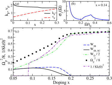
Figure 2: (Color online) (a) The Fermi wavevector $k_{F}$ and velocity $v_{F}$ in the nodal direction for the YRZ dispersion. These are given in units of $1/a$ and $t_{0}a/\hbar$, respectively. (b) The real part of the optical conductivity (arbitrary units) in the pseudogapped normal state as a function of $\Omega/t_{0}$, illustrating the Drude and interband components. (c) A plot comparing the plasma frequency $\Omega_{p}^{2}$ and the square of the inverse penetration depth. Also, shown are the Drude and interband optical spectral weights, $W_{D}$ and $W_{IB}$ as a function of doping $x$ and the interband spectral weight in the superconducting state $W_{IB,SC}$. For all of these quantities shown here we have left out the doping-dependent prefactor $g_{t}^{2}$. These curves are all in units of $e^{2}t_{0}/\hbar^{2}d$, where $d$ is the $c$-axis distance per Cu-O plane.

We begin with a discussion of the validity (or lack thereof) of this rule in the YRZ model. We will work only at $T=0$ which is simplest and where the superconducting gap is fully developed and so has its maximum effect on charge dynamics. Thus we would expect that, if the presence of the pseudogap leads to a violation of Eq. (23), it should be most noticeable here. In Fig. 2(c), we plot several of the relevant quantities as a function of doping, $x$. The solid black dots give $\Omega_{p}^{2}/8$, i.e., the right hand entry of Eq. (23). The change in behavior at $x=0.2$ corresponds to the QCP in our phase diagram and signals the emergence of a finite pseudogap. Since we are in the clean limit, and also in the normal state, $\Omega_{p}^{2}/8$ corresponds to $W_{D}/2$ (green dash-double-dotted curve) in the Fermi liquid region of the phase diagram $x\geq 0.2$. Below this doping, $\Omega_{p}^{2}/8$ has two contributions $W_{D}/2$ from the Drude peak and $W_{IB}$ (long-dashed blue curve) from the interband transitions. A plot which illustrates the two contributions to ${\rm Re}\sigma(T=0,\Omega)$ is shown in Fig. 2(b). For this plot we used a formula for the conductivity which included elastic impurity scattering with quasiparticle scattering rate $\eta$ set equal to $0.01t_{0}$. While the Drude and interband contributions are not completely separated, the two distinct contributions remain clearly identified. The Drude is centered about $\Omega=0$ and the interband piece is shifted to higher energies with an onset just above $\Omega=0.2t_{0}$. The plot is for doping $x=0.14$. This is a case where the pseudogap is larger than the superconducting gap with $\Delta_{\rm pg}/t_{0}=0.18$ which corresponds roughly to the onset mentioned above. Returning to Fig. 2(c), the sum of $W_{D}/2$ and $W_{IB}$ add up to $\Omega_{p}^{2}/8$ in the normal state. As we have already mentioned, in the superconducting state at zero temperature in the clean limit, the entire Drude condenses into the superfluid and there is no contribution to the optical spectral weight $\int_{0^{+}}^{\infty}{\rm Re}\sigma_{S}(T=0,\Omega)d\Omega$ from this term, only the interband term remains. Its value as a function of doping is denoted by $W_{IB,SC}$ and is given by the solid black curve. Comparing this with its normal state value (long-dashed blue curve), we see that at doping just below the QCP at $x=0.2$, this contribution is very small and so most of $W_{IB}$ also goes into the condensate. However, as $x$ decreases towards the more underdoped regime, much less of $W_{IB}$ condenses and by $x\simeq 0.1$, this condensation has stopped. This behavior is expected and shows that the interband piece is less susceptible to condensation into Cooper pairs than is the Drude and that this trend increases rapidly as the pseudogap energy becomes large as compared with twice the superconducting gap energy. In our phase diagram, this boundary comes at about $\sim 0.1$ doping as we would expect.

The dot-double-dashed purple curve gives $1/8\lambda(0)^{2}$. When this is added to $W_{IB,SC}$, we obtain, within our numerical accuracy, the $\Omega^{2}_{p}/8$, i.e., the solid black circles. Thus we find that to this precision, the YRZ model also satisfies Eq. (23) which is one of our important results about optical spectral weight distribution in addition to our observation that little of the interband contribution to the conductivity condenses into Cooper pairs when $\Delta^{0}_{\rm sc}$ becomes small as compared to the pseudogap $\Delta^{0}_{\rm pg}$. Finally, in Fig. 2(a), we show our results for the Fermi momentum in the nodal direction (solid black curve) as well as the corresponding Fermi velocity (dashed red curve). Our values agree well with those given in the work of YRZ and will be needed in a following section.

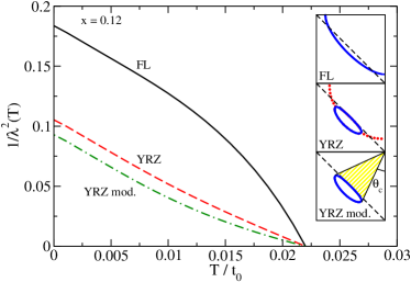
Figure 3: (Color online) The temperature dependence of the penetration depth shown as $1/\lambda^{2}(T)$ versus $T/t_{0}$. Here, the $g^{2}_{t}$ prefactor, that arises from the definition of the coherent part of the Green’s function, is included. Shown are curves for the Fermi liquid state (FL, solid black curve) and the modification which occurs when a pseudogap is present in the YRZ model (red dashed curve). The curve labeled YRZ mod. (green dash-dotted) is a modification of the YRZ model where the superconducting gap is only non-zero on the Fermi pocket. The three Fermi surfaces involved are illustrated schematically in the inset (see text) including the critical angle $\theta_{c}$.

V Results

We will now present in detail our results and analysis for the penetration depth. Note that up until now, in our formulas and discussion, we have not included the Gutzwiller $g_{t}$ prefactor for weighting only the coherent part of the Green’s function in Eq. (1). Due to the product of two spectral functions that enters the formulas for the penetration depth and the optical conductivity [Eq. (LABEL:eq:BB) and Eq. (17), respectively], $1/\lambda^{2}(T)$ and $\sigma(T,\Omega)$ will include a doping-dependent prefactor of $g_{t}^{2}$. We now include it from here on forward as this factor reflects the highly correlated nature of the cuprates and is necessary for a proper comparison with experiment.

In Fig. 3, we present our results for the temperature dependence of the penetration depth for $x=0.12$. Three cases are considered and are to be compared. The solid black curve labeled Fermi liquid is obtained when the pseudogap is set equal to zero and is for comparison with the short-dashed red curve which includes the pseudogap and is labeled YRZ. We note two striking differences between these two sets of results. First, as a function of temperature, the FL curve shows concave down behavior. This differs slightly from the perhaps more classical curve for a $d$-wave superconductor in a model, where the continuum approximation is used for the band structure and a $\cos(2\theta)$ gap variation is assumed on the cylindrical Fermi surface, but is mainly due to our use of a gap ratio of $2\Delta_{\rm sc}^{0}/k_{B}T_{c}=6$ rather than the weak coupling BCS $d$-wave value of 4.28. The use of a larger value for this ratio is in keeping with experimental observation that finds it of order of 6 (and occasionally reported to be even larger). Our results also represent a generalization in which the superconducting gap varies over the entire Brillouin zone and the band structure is given in tight-binding with up to third nearest neighbor hopping. The same gap and bands are used for the red dashed curve which by contrast shows slight concave upward variation as a function of temperature. Here a pseudogap is included and this has changed the usual large Fermi surface of Fermi liquid theory which is shown in one quadrant of the Brillouin zone in the top inset, to the Fermi surface shown in the middle inset. Here, the blue curve is the Luttinger pocket of the YRZ theory and the red line is its shadow extension which represents a momentum contour of minimum approach to the “Fermi surface” in regions of momentum space where a gap exists so there are no true zero energy states. This reconstruction of the Fermi surface into a Luttinger pocket, which by its construction contains exactly $x$ empty states (holes), has led to a large suppression of the zero temperature penetration depth as expected in our simplified Eq. (16). The second striking feature of these two curves is that they have identical values of slope, as a function of temperature $T$, out of $T=0$. The formation of the Luttinger pockets, as the pseudogap increases in the underdoped regime of $x$ below the QCP at $x=0.2$ in our phase diagram, reduces the amount of Fermi surface that is available for pairing as in other competing order parameter scenariossharapov , but leaves the nodal region ungapped. The very low temperature excitations out of the ground state are confined to the cone very near zero energy, which exists in the nodal direction only, but these excitations do not sample directly the pseudogap and so the slope retains its Fermi liquid value.

The final curve in Fig. 3 (green dash-dotted) is a case where we have cut off the superconducting gap outside the solid angle $1-4\theta_{c}/\pi$ which defines the region of the Luttinger pocket, with $\theta_{c}$ shown in the lower inset. As we expect from the above arguments this does not change the low temperature slope but does affect the zero temperature value of the superfluid stiffness which is further reduced over its Fermi liquid value. Our motivation for applying this cutoff is the expectation that the superconducting gap will form mainly on the part of the Fermi surface which remains ungapped. This idea is consistent with recent ARPES dataarpes and will be discussed further in a future paperjamesarpes .

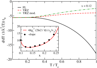
Figure 4: (Color online) Plot of slope of the penetration depth curves shown in Fig. 3 versus $T/T_{c}$. The inset shows a comparison of the magnitude of the slope as $T\to 0$ with the formula $4\pi g_{t}^{2}[2\ln 2/\pi](v_{F}/v_{\Delta})$. This expression (solid line) is shown tested against the numerical data (dots) as a function of doping $x$.

Figure 4 further emphasizes the insensitivity of the low temperature slope of $1/\lambda^{2}(T)$ to the formation of the Luttinger pockets and any cut off in the superconducting gap away from the nodal region. Shown in Fig. 4 is $t_{0}d/dT[1/\lambda^{2}(T)]$ vs $T/T_{c}$ for the three cases illustrated in Fig. 3. The line labels are the same. We see perfect agreement between the three curves below $T/T_{c}\sim 0.3$. With increasing temperature, the Fermi liquid case shows a downward trend while by contrast the two other non-Fermi liquid curves show the opposite. In the inset to the figure we show our results for the slope in the YRZ model (solid black dots) as a function of doping. Also shown for comparison is the formula

$$t_{0}\frac{d}{dT}\biggl{[}\frac{1}{\lambda^{2}(T)}\biggr{]}=4\pi g_{t}^{2}\frac{2\ln 2}{\pi}\frac{v_{F}}{v_{\Delta}},$$ (24)

where $v_{\Delta}=|\nabla\Delta_{\rm sc}(k)|_{k_{F}}=(\Delta^{0}_{\rm sc}/\sqrt{2})|\sin(k_{Fx})|$, with all quantities defined in terms of the units stated in Fig. 2 and elsewhere. Here, the $|\sin(k_{Fx})|$ factor accounts for the fact that the superconducting gap amplitude sampled on the Luttinger pocket is somewhat smaller than the input value $\Delta^{0}_{\rm sc}$ which enters the phase diagram and corresponds to the maximum gap in the Brillouin zone. Formula (24) is derived for a Fermi liquid with general band structure and we see here that it also applies to YRZ theory (Fig. 4).

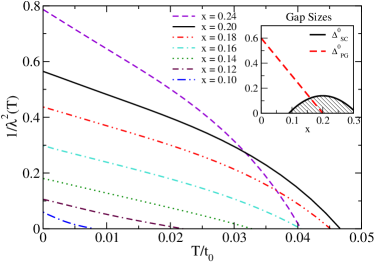
Figure 5: (Color online) The temperature dependence of the inverse square of the penetration depth for various dopings. The inset shows the values of the superconducting gap and pseudogap in units of $t_{0}$ for varying doping parameter $x$.

In Fig. 5, we show $1/\lambda^{2}(T)$ vs $T/t_{0}$ for different values of doping $x$. The phase diagram identifying the superconducting gap and pseudogap values used is shown for reference in the inset where we see the QCP at $x=0.2$ corresponding to the onset of a finite pseudogap which progressively modifies the large Fermi surface of Fermi liquid theory to smaller Luttinger pockets. Several overall trends displayed in the $1/\lambda^{2}(T)$ curves shown in this figure are in qualitative agreement with two recent data sets, one for highly underdoped YBa₂Cu₃O_6+y (YBCO)broun ; sfuubc and the other for the Bi-based cuprates (Bi:2212) Bi_2.15Sr_1.85CaCu₂O_8+δ and Bi_2.1Sr_1.9Ca_0.85Y_0.15Cu₂O_8+δ (Ref. anukool ). In addition to the reduction in the $T=0$ value of $1/\lambda^{2}(T)$, there is also a trend for the linear temperature dependence out of $T=0$ to remain to higher values of reduced temperature $T/T_{c}$. This contrasts with the concave downward behavior seen in overdoped and optimally doped casesbonnhardy as $T_{c}$ is approached. Such a trend towards linearity is clearly seen in the data of Huttema et al.sfuubc ; broun who note a near linear dependence of the data almost all the way to $T_{c}$. However, they also find, in Fig. 3 of their paper, a turnaround to a $T^{2}$ law at low temperatures in agreement with the well-known effect of impurities in $d$-wave superconductors. While we have not included impurities in our work, we expect no modifications to this law to arise in the YRZ model and so agree with these results. However, because the YBCO data is in the deeply underdoped regime near the bottom of the superconducting dome, there could be additional effects that become important such as fluctuations,lemberger not included here. Hence we turn to the data of Anukool et al.anukool on Bi:2212 and in particular their Fig. 3(b) which, in agreement with our findings, shows near linear behavior over the entire temperature range considered. Similar behavior is also seen in their purer sample (shown in their Fig. 3(a)) although in that case the overdoped samples show a low temperature upturn which may indicate physics not included here. The Bi:2212 data set will be examined more closely in what follows as the doping range is more compatible with the assumptions of the YRZ model.

In Fig. 6, we show our results for the value of the zero temperature penetration depth as a function of doping $x$ for three models. The solid black circles are based on a Fermi liquid model for the renormalized band which includes the Gutzwiller factors of the YRZ theory but no pseudogap. We see a smooth evolution with increasing superfluid density as doping increases. The solid red squares are for comparison and include the pseudogap which is finite below the QCP. A finite $\Delta_{\rm pg}$ leads to Fermi surface reconstruction as shown in the insets of Fig. 3 where the Luttinger pockets are seen in the middle and lower frame and are to be compared with the large Fermi liquid Fermi surface of the top panel. For $x$ just below the QCP, the Fermi surface reconstruction can be even more complex than in Fig. 3. An example is shown in the inset of Fig. 6 for $x=0.18$, where we show Luttinger surface with the dashed curve being the AFBZ boundary. Note the pieces of occupied $\bm{k}$-space on the other side of the AFBZ boundary. In the main frame, the solid green diamonds include the pseudogap and, in addition, the superconducting gap is assumed to be non-zero only on the Luttinger pocket in an attempt to make the calculations more realistic. As we saw in Eq. (16) with a simplified continuum model for the band structure, we expect $1/\lambda^{2}(0)$ to drop as the Fermi surface arc is reduced because the size of the Luttinger pocket shrinks. The solid black curve corresponds to the product of the Fermi liquid value of $1/\lambda^{2}(0)$ with the factor $1-4\theta_{c}/\pi$, the latter gives an approximate measure of the ratio of the angle of the remaining Fermi arc compared with that for the Fermi liquid. This curve follows the same general trend as do the results of detailed calculations. This shows that Fermi surface reconstruction is responsible for the drop in solid green diamonds below the Fermi liquid values (solid black circles). We note again in this regard that as the QCP is approached from below ($x<0.2$), there is a region where the Fermi surface reconstruction is complex (see insert) and is not easily characterized by a single arc length. Here, we use the values previously derived within the context of an application of the YRZ model to the specific heatjames . This explains why the solid black line starts to deviate from the solid green diamonds in the region near the QCP. We emphasize that the solid green diamonds include a cut off on the superconducting gap.

As can be seen in the approximate qualitative formula (16), we expect the superconducting gap to affect the zero temperature condensate, a result which is quite different from the Fermi liquid case where $1/\lambda^{2}(0)$ depends only on normal state parameters and not on the gap. Recently Kopnin and Soninkopnin found a similar dependence on superconducting gap in the case of graphene although no superconductivity has yet been reported in this system even though carbon nanotubes have been found to superconduct.nanotubes Returning to Eq. (16), the correction factor of $c\equiv(-4\theta_{c}/\pi)(\Delta^{0}_{\rm pg})^{2}/[(\Delta_{\rm sc}^{0})^{2}+(\Delta_{\rm pg}^{0})^{2}]$ reduces to $-4\theta_{c}/\pi$ only when $\Delta_{\rm sc}^{0}$ is assumed to be zero when $\Delta^{0}_{\rm pg}$ is finite, the case described so far. If the superconducting gap is allowed to exist over the entire Fermi surface, the correction factor $c$ will be less than $-4\theta_{c}/\pi$ and we get the blue dash-dotted curve in Fig. 6 as the product of $(1-c)$ times the Fermi liquid value of $1/\lambda(0)^{2}$ [i.e., Eq. (16)]. This curve agrees well with the solid red squares which are obtained from the full calculations. It is clear that Fermi surface reconstruction leads to a strong reduction of the zero temperature superfluid density as a result of the loss of ungapped states on the Fermi surface.

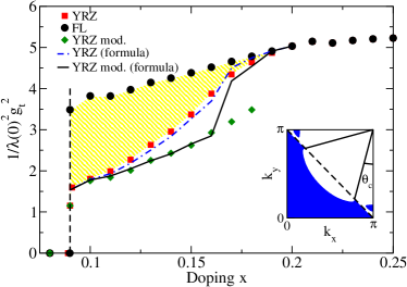
Figure 6: (Color online) The $T=0$ inverse square penetration depth as a function of doping, comparing the cases of the Fermi liquid (FL), YRZ and the modified YRZ ansatz. The shade region emphasizes the reduction in this quantity due to Fermi surface reconstruction. The curves are for simple analytic formulas as discussed in the text. The inset shows the Luttinger area (shaded blue) for the case of $x=0.18$, illustrating an intermediate regime of the Fermi surface reconstruction as a function of doping. This inset also illustrates the critical angle $\theta_{c}$ for defining the Fermi pocket, which has become ill-defined in this case.

We now turn to experiment to assess the validity of the theoretical model due to YRZ. Recent results as a function of doping on the penetration depth of Bi-based cuprates (Bi:2212) have been published by Anukool et al.anukool . They give results for a range of doping from underdoped to overdoped and for $T_{c}$’s reduced by up to 50%. Because their optimal doping is at $p=0.16$ and our model uses $x=0.2$, we shifted the data set doping values by 0.04 in order to match their dome with ours. Normalizing to the optimal doping, we then find that their $T_{c}$ curve matches our $T_{c}$ dome if we convert our energy gap dome to one for $T_{c}$ by using a value of the gap ratio $2\Delta^{0}_{\rm sc}/k_{B}T_{c}=6$ and then taking $t_{0}=165$ meV (our energy units have all been in units of $t_{0}$). With this we find a good match to the experimental $T_{c}$ versus doping curve shown in Fig. 7. This now fixes our parameters for the rest of our work. In Fig. 7 (right hand frame) we show the classic Uemura plot of $T_{c}$ versus $1/\lambda^{2}(0)$, where we have normalized our results and the data to the value at optimal doping. The agreement with the data is excellent and on the underdoped side, the data appears to favor more the modified YRZ calculation.

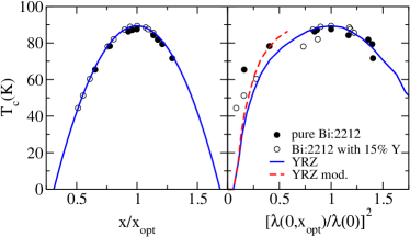
Figure 7: (Color online) $T_{c}$ vs doping and vs the superfluid density normalized to the optimal value in the YRZ model. The solid blue curve is the result of the YRZ model and the red dashed curve is the modified YRZ model as discussed in the text. Comparison has been made with the data of Anukool et al.anukool with the Bi:2212 (solid dots) and Bi(Y):2212 (open dots).

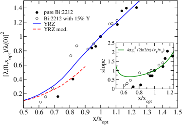
Figure 8: (Color online) Comparison of the superfluid density at $T=0$ with the Bi:2212 (solid dots) and Bi(Y):2212 (open dots) data of Anukool et al.anukool . This is shown as a function of doping scaled to the optimal doping value. The solid blue curve is the result of the YRZ model and the red dashed curve is the modified YRZ model as discussed in the text. The inset shows the slopes of the data as $T\to 0$ in comparison with the analytic formula discussed in Fig. 4.

Furthermore, in Fig. 8, we show the data compared with the inverse penetration depth squared versus doping and once again the data favors the modified YRZ curve. What is clear here is that the data agrees well with the Fermi liquid curve above optimal doping and on the underdoped side it follows the YRZ curve which includes the reconstructed Fermi surface. Indeed, the drop in the data below optimal doping can be taken as possible indirect experimental evidence for Fermi surface reconstruction as the Fermi liquid curve would have been higher (as discussed in relation to Fig. 6). All is not ideal, however. We have used a normalized quantity here. In absolute value, we find that the superfluid density is off by about a factor of 3-4. Nonetheless, this can be rectified as the penetration depth depends only on $t_{0}$ and so one could increase the value of $t_{0}$ to account for this. This would then require an adjustment of the gap ratio to keep the good agreement with the $T_{c}$ dome of Fig. 7, but we find that it would be unrealistically large. Another possibility is to note that our estimate of the Fermi velocity in the YRZ model at optimum is low by a factor of two. The superfluid density shown here goes as the square of the velocity and this could possibly correct the situation. A related issue is that the band structure used in the YRZ paper is for a very different compound than that of Bi:2212 and so this could change some of these quantitative numbers. We wish to stress that the merit of this theory should be seen in its ability to give qualitative insight into the pseudogap phase and the good agreement that we find here is very encouraging given the lack of detailed parameter fitting to this particular material. Also shown in Fig. 8 is an inset plotting the experimental slope of the inverse square penetration depth curves for $T\to 0$. Again this has been normalized to the optimal doping value and we find good agreement with the analytic formula discussed for the slope in Fig. 4. An analysis based on ARPES has given somewhat different results.norman It should be noted that we extracted the slope values ourselves and so this is not a rigorous representation of the data and indeed the temperature-dependence of some of the experimental curves was unusual in a few cases, but we took the lowest temperature value of the slope in any event. The optimal doping curve was in this category as it showed an upturn at low temperature in the case of the pure sample and so its slope value and a few of the others could be revised in the hands of experimental experts. However, the inset of Fig. 8 (as well as the other comparisons of Figs. 7 and 8) serves to illustrate that the Gutzwiller prefactor for the coherent part of the Green’s function, leading to a prefactor of $g_{t}^{2}$, appears to be essential in giving the correct trend of the data with doping. This points to very strong correlations in these systems.

Figure 9: (Color online) A comparison of the effect that various models have on the square of the inverse penetration depth as a function of temperature. The schematic diagrams illustrate the momentum dependence of the two energy gaps for the Fermi arc model and its modification, relative to the nodal liquid case.

In Fig 9, we give results which show the relationship of the YRZ model with two other prominent models. Both involve the assumption that the pseudogap acts on the Fermi surface. This corresponds to taking the limit of $\xi^{0}_{\bm{k}}\to\xi_{\bm{k}}$ in our Eq. (9) for the penetration depth, i.e., to replacing the AFBZ energy by the carrier dispersion curve. As we saw, this greatly simplifies the equation and reduces it to the familiar form of Eq. (LABEL:eq:bpen) for a BCS superconductor with one modification. While in Eq. (LABEL:eq:bpen) the superfluid density remains directly proportional to a factor of $\Delta^{2}_{\rm sc}$ and so manifestly vanishes in the normal state, the energy $E_{S}=\sqrt{\xi_{\bm{k}}^{2}+\Delta^{2}_{\rm sc}+\Delta^{2}_{\rm pg}}$ involves the sum of the squares of $\Delta_{\rm sc}$ and $\Delta_{\rm pg}$ rather than the square of $\Delta_{\rm sc}$ alone. It is only through this factor that the pseudogap enters in this simplification. The Fermi arc modeljames corresponds to taking $\Delta_{\rm pg}$ non-zero only on an arc centered about the antinodal direction, leaving an ungapped region centered around the nodal direction (on the Luttinger pocket) as illustrated by the center insert in Fig. 9. One can construct realistic modelsstorey for the momentum variation of the pseudogap on the Fermi surface. For simplicity, here we retain its cosine form $\Delta_{\rm pg}=\frac{\Delta_{\rm pg}^{0}(x)}{2}(\cos k_{x}a-\cos k_{y}a)$ but cut it off on an arc defined by the angle $\theta_{c}$ previously introduced. Taking $\theta_{c,\rm arc}=24^{\circ}$, chosen to get a best fit to the penetration depth curve of the YRZ model (solid black curve), one obtains the red open circles which overlap the black solid curve almost perfectly. Thus with the right choice of $\theta_{c,\rm arc}$, one can get an almost perfect match between the two models. If we further assume that the superconducting gap is present only on the ungapped (by the pseudogap that is, see right hand inset) part of the Fermi surface, we obtain the dashed curve denoted Arc mod. This has pushed the penetration depth down by about the same amount as we saw in Fig. 3 for the full YRZ calculation when we included a superconducting gap modification in this model. The choice of $\theta_{c,arc}$ in Fig. 9 is important as can be seen from the dash-dotted blue curve which is also based on an arc model but with a different cut off model $\theta_{c,\rm YRZ}=26^{\circ}$, a value obtained from the size of the arc subtended by the actual Luttinger pocket of the YRZ theory. While this choice decreases further the magnitude of the superfluid density because there is even less ungapped arc, it does not change the qualitative behavior obtained.

Finally, the solid green curve with triangles is our result for the nodal liquid which corresponds to lifting the cut off on the pseudogap. In this case an effective gap of $\sqrt{\Delta_{\rm sc}^{2}+\Delta_{\rm pg}^{2}}$ replaces the usual superconducting gap in the standard Eq. (LABEL:eq:bpen) for $1/\lambda^{2}(T)$ with one critical difference. In the numerator of Eq. (LABEL:eq:bpen), it is still $\Delta_{\rm sc}^{2}$ which remains and not $\Delta_{\rm sc}^{2}+\Delta_{\rm pg}^{2}$. Since we have assumed the same momentum dependence for the superconducting gap and pseudogap, we can replace the explicit $\Delta_{\rm sc}^{2}$ factor in Eq. (LABEL:eq:bpen) by $\Delta_{\rm sc}^{2}+\Delta_{\rm pg}^{2}$ and take out the factor of $(\Delta_{\rm sc}^{0})^{2}/[(\Delta_{\rm sc}^{0})^{2}+(\Delta_{\rm pg}^{0})^{2}]$ to compensate for this. Thus the equation for the penetration depth becomes the standard one for an effective superconducting gap of $\sqrt{\Delta_{\rm sc}^{2}+\Delta_{\rm pg}^{2}}$ but with the difference that a factor of the square of superconducting-to-effective-gap amplitude is to multiply the entire expression as we see explicitly in our simplified expression (14). While these simplifications allow us to obtain simple analytic expressions, we see that this limit fails to give quantitative results when compared with YRZ. Compare the green curve with triangles with the solid black curve in Fig 9. In fact one should not expect the two models to agree. The nodal liquid is the limit when the size of the Luttinger pocket tends to zero. But this is never reached inside the superconducting dome. In our calculations at a doping where $T_{c}$ has been depressed to zero, there remains a sizable part of the Fermi surface which is ungapped. It is not surprising then that the nodal liquid should show qualitative behavior not part of the arc model, such as, a superfluid density at $T=0$ which decreases by a factor of the square of the ratio of superconducting to pseudogap. The slope of the linear-in-$T$ variation at low temperature also becomes inversely proportional to $\sqrt{\Delta_{\rm pg}^{2}+\Delta_{\rm sc}^{2}}$ rather than to $\Delta_{\rm sc}$ and so becomes very flat.

VI Conclusions

YRZ have provided a simple model for the coherent part of the charge carrier Green’s function which applies below a quantum critical point characterizing the beginning of pseudogap formation. As the Mott-Hubbard transition to an insulating state is approached with decreasing doping, the magnitude of the pseudogap increases, the bands narrow and the weight of the coherent piece of the Green’s function decreases according to well-defined Gutzwiller factors which account for correlation effects. With increasing pseudogap magnitude, the Fermi surface reconstructs. It goes from the large Fermi surface of Fermi liquid theory to ever smaller Luttinger pockets. This leads directly to a reduction of the value of the zero temperature inverse squared penetration depth because there are fewer ungapped states which are available to form the condensate. We show that this reduction is roughly proportional to the ratio of the remaining arc length, defined by the Luttinger pocket, to the full length of the corresponding Fermi liquid surface. On the other hand, and in sharp contrast, the coefficient of the linear-in-temperature term of $1/\lambda^{2}(T)$ at small $T$ remains largely unaffected because this quantity depends only on the available very low energy excitations and these are confined to the vicinity of the nodal Dirac points. This region is not importantly affected by pseudogap formation and implied Fermi surface reconstruction.

A comparison of our results with recent experimental data on Bi:2212 gives good qualitative agreement and demonstrates the importance of the strong dependence on doping of the coherence weight in the YRZ model which derives from strong correlation effects. While this is a simple multiplicative factor, it accounts for a significant part of the reduction in superfluid density as the end of the superconducting dome is approached in the deeply underdoped region of the phase diagram. An additional reduction is due to Luttinger pocket formation which starts at the doping associated with the quantum critical point and this effect provides a more abrupt change in magnitude which should be measurable as a signature of Fermi surface reconstruction.

The well-known Ferrell-Glover-Tinkham sum rule of conventional superconductivity was found to apply here as well. The optical weight lost on entering the superconducting state below $T_{c}$ reappears in its entirety in the superfluid fraction.

Comparison of our results with those based on an arc model, with pseudogap placed on the Fermi surface rather than on the AFBZ of the YRZ model, can be made to agree very well if the arc length on which the pseudogap is assumed to be non-zero is appropriately chosen to obtain a best fit with the YRZ case. The nodal liquid concept corresponds to the limit when the Fermi surface is fully gapped by the pseudogap except for the nodal points. This limit is never reached in YRZ theory because the size of the Luttinger pocket remains quite significant at the doping which corresponds to the end of the superconducting dome. Nevertheless, the nodal liquid limit remains valuable because it yields analytic results which can provide useful insight into the deeply underdoped case.

- (1) T. Timusk and B. Statt, Rep. Prog. Phys. 62, 61 (1999).
- (2) See J.P. Carbotte, E. Schachinger, and D. N. Basov, Nature (London) 401, 354 (1999) and references therein.
- (3) E. Schachinger and J. P. Carbotte, Phys. Rev. B 62, 9054 (2000).
- (4) S. Chakravarty, R. B. Laughlin, D. K. Morr, and C. Nayak, Phys. Rev. B 63, 094503 (2001).
- (5) V. J. Emery and S. A. Kivelson, Nature (London) 374, 434 (1995).
- (6) M. Randeria, N. Trivedi, A. Moreo, and R. T. Scalettar, Phys. Rev. Lett. 69, 2001 (1992).
- (7) G. Alvarez and E. Dagotto, Phys. Rev. Lett. 101, 177001 (208).
- (8) Q. Chen, K. Levin, and I. Kosztin, Phys. Rev. B 63, 184519 (2001).
- (9) S. Hüfner, M. A. Hossain, A. Damascelli, and G. A. Sawatzky, Rep. Prog. Phys. 71, 062501 (2008).
- (10) H. v. Löhneysen, A. Rosch, M. Vojta, and P. Wölfe. Rev. Mod. Phys. 79, 1015 (2007).
- (11) L. Taillefer, arXiv:0901.2313 and references therein.
- (12) For example, A. Kanigel, U. Chatterjee, M. Randeria, M. R. Norman, S. Souma, M. Shi, Z. Z. Li, H. Raffy, and J. C. Campuzano, Phys. Rev. Lett. 99, 157001 (2007); A. Kanigel, M. R. Norman, M. Randeria, U. Chatterjee, S. Souma, A. Kaminski, H. M. Fetwell, S. Rosenkranz, M. Shi,T. Sato, T. Takahashi, Z. Li, H. Raffy, K. Kadowaki, D. Hinks, L. Ozyuzer, and J. C. Campuzano, Nat. Phys. 2, 447 (2006); T. Kondo, R. Khasanov, T. Takluchi, J. Schmalian, and A. Kaminski, Nature (London) 457, 296 (2009).
- (13) J. Meng, G. Liu, W. Zhang, L. Zhao, H. Liu, X. Jia, D. Mu, S. Liu, X. Dong, W. Lu, G. Wang, Y. Zhou, Y. Zhu, X. Wang, Z. Xu, C. Chen, and X. J. Zhou, arXiv:0906.2682
- (14) J. Hwang, J. P. Carbotte, and T. Timusk, EPL 82, 27002 (2008).
- (15) J. G. Storey, J. L. Tallon, G. V. M. Williams, and J. W. Loram, Phys. Rev. B 76, 060502(R) (2007).
- (16) Y. Kohsaka, C. Taylor, P. Wahl, A. Schmidt, Jhinhwan Lee, K. Fujita, J. W. Alldredge, Jinho Lee, K. McElroy, H. Esaki, S. Uchida, D.-H. Lee, and J. C. Davis, Nature (London) 454, 1072 (2008).
- (17) K.-Y. Yang, T. M. Rice and F. C. Zhang Phys. Rev. B 73, 174501 (2006).
- (18) P. W. Anderson, Science 235, 1196 (1987).
- (19) B. Valenzuela and E. Bascones, Phys. Rev. Lett. 98, 227002 (2007).
- (20) E. Illes, E. J. Nicol, and J. P. Carbotte, Phys. Rev. B 79, 100505(R) (2009).
- (21) K.-Y. Yang, H. B. Yang, P. D. Johnson, T. M. Rice and F. C. Zhang, EPL 86, 37002 (2009).
- (22) J. P. F. LeBlanc, E. J. Nicol, and J. P. Carbotte, Phys. Rev. B 80, 060505(R) (2009).
- (23) W. N. Hardy, D. A. Bonn, D. C. Morgan, R. Liang, and K. Zhang, Phys. Rev. Lett. 70, 3999 (1993).
- (24) Y. Uemura et al., Phys. Rev. Lett. 62, 2317 (1989).
- (25) P. A. Lee and X.-G. Wen, Phys. Rev. Lett. 78, 4111 (1997).
- (26) D. E. Sheehy, T. P. Davis, and M. Franz, Phys. Rev. B 70, 054510 (2004).
- (27) D. Branch and J. P. Carbotte, Phys. Rev. B 52, 603 (1995).
- (28) P. G. Tomlinson and J. P. Carbotte, Phys. Rev. B 13, 4738 (1976).
- (29) H. K. Leung, J. P. Carbotte, D. W. Taylor, and C. R. Leavens, Can. J. Phys. 54, 1585 (1976).
- (30) H. K. Leung, J. P. Carbotte, and C. R. Leavens, J. Low Temp. Phys. 24, 25 (1976).
- (31) D. Branch, Ph.D. thesis, McMaster University, 1997 (unpublished)
- (32) R. J. Radtke, V. N. Kostur, and K. Levin, Phys. Rev. B 53, R522 (1996).
- (33) E. Schachinger, J. P. Carbotte, and F. Marsiglio, Phys. Rev. B 56, 2738 (1997).
- (34) C. O’Donovan and J. P. Carbotte, Phys. Rev. B 52, 16208 (1995).
- (35) C. O’Donovan and J. P. Carbotte, Phys. Rev. B 52, 4568 (1995).
- (36) C. O’Donovan and J. P. Carbotte, Physica C 252, 9433 (1996).
- (37) S. Misawa, Phys. Rev. B 51, 11791 (1995).
- (38) R. A. Ferrell and R. E. Glover, Phys. Rev. 109, 1398 (1958).
- (39) M. Tinkham and R. A. Ferrell, Phys. Rev. Lett. 2, 331 (1959).
- (40) S. G. Sharapov and J. P. Carbotte, Phys. Rev. B 73, 094519 (2006).
- (41) T. Kondo, R. Khasanov, T. Takeuchi, J. Schmalian, and A. Kaminski, Nature (London) 457, 296 (2009).
- (42) J. P. F. LeBlanc, J. P. Carbotte, and E. J. Nicol, (unpublished).
- (43) D. M. Broun, W. A. Huttema, P. J. Turner, S. Özcan, B. Morgan, R. Liang, W. N. Hardy, and D. A. Bonn, Phys. Rev. Lett. 99, 237003 (2007).
- (44) W. A. Huttema, J. S. Bobowski, P. J. Turner, R. Liang, W. N. Hardy, D. A. Bonn, and D. M. Broun, Phys. Rev. B 80, xxx (2009).
- (45) W. Anukool, S. Barakat, C. Panagopoulos, and J. R. Cooper, Phys. Rev. B 80, 024516 (2009).
- (46) I. Hetel, T. R. Lemberger, and M. Randeria, Nature Phys. 3, 700 (2007).
- (47) N. B. Kopnin and E. B. Sonin, Phys. Rev. Lett. 100, 246808 (2008).
- (48) Z. K. Tang, Lingyun Zhang, N. Wang, X. X. Zhang, G. H. Wen, G. D. Li, J. N. Wang, C. T. Chan, and Ping Sheng, Science 292, 2462 (2001).
- (49) J. Mesot, M. R. Norman, H. Ding, M. Randeria, J. C. Campuzano, A. Paramekanti, H. M. Fretwell, A. Kaminski, T. Takeuchi, T. Yokoya, T. Sato, T. Takahashi, T. Mochiku, and K. Kadowaki, Phys. Rev. Lett. 83, 840 (1999).