Computational Geometric Optimal Control of
Connected Rigid Bodies in a Perfect Fluid

Abstract

This paper formulates an optimal control problem for a system of rigid bodies that are connected by ball joints and immersed in an irrotational and incompressible fluid. The rigid bodies can translate and rotate in three-dimensional space, and each joint has three rotational degrees of freedom. We assume that internal control moments are applied at each joint. We present a computational procedure for numerically solving this optimal control problem, based on a geometric numerical integrator referred to as a Lie group variational integrator. This computational approach preserves the Hamiltonian structure of the controlled system and the Lie group configuration manifold of the connected rigid bodies, thereby finding complex optimal maneuvers of connected rigid bodies accurately and efficiently. This is illustrated by numerical computations.

I Introduction

Fish locomotion involves a deformable fish body interacting with an unsteady fluid, through which internal muscular forces on the fish are translated into fish motions [1].

The planar articulated rigid body model has become popular in engineering, as it describes underwater robotic vehicles that move and steer by changing their shape [2]. Furthermore, if it is assumed that the ambient fluid is incompressible and irrotational, then equations of motion of the articulated rigid body can be derived without explicitly incorporating fluid variables [3]. The effect of the fluid is accounted by added inertia terms of the rigid body. This model is known to characterize the qualitative behavior of fish swimming [3].

In [4], an analytical model and a geometric numerical integrator for three-dimensional connected rigid bodies immersed in an incompressible and irrotational fluid were developed. The connected rigid bodies can freely translate and rotate in three-dimensional space, and each joint has three rotational degrees of freedom. The geometric numerical integrator presented in [4] is referred to as a Lie group variational integrator [5], and it preserves the symplecticity, momentum map, and Lie group configuration manifold of the connected rigid bodies. These properties are important for accurately and efficiently studying complex maneuvers of rigid bodies [6].

This paper formulates an optimal control problem for connected rigid bodies in a perfect fluid. We assume that internal control moments are applied at each joint. These control moments change the relative attitude between rigid bodies, thereby controlling the shape of a system of connected rigid bodies. By using the nonlinear coupling, referred to as a geometric phase [7], between shape changes and group motions, and by using the momentum exchange between the rigid bodies and the ambient fluid, the system of connected rigid bodies can translate and rotate without external forces or moments.

We present a computational approach to solve optimal control problems based on the Lie group variational integrators developed in [4]. The optimal control problems are formulated as discrete-time optimal control problems using Lie group variational integrators; these problems can be solved using standard numerical optimization techniques. This is in contrast to conventional approaches where discretization is introduced at the last stage in order to solve the optimality conditions numerically.

This computational geometric optimal control approach preserves the Hamiltonian structure of the controlled system and Lie group structure of connected rigid bodies in fluid [8]. As it does not introduce artificial numerical dissipation that typically appear in general-purpose numerical integration methods, it improves the overall computational efficiency and accuracy of the optimization process. As it is coordinate-free, this approach avoids singularities and complexities associated with local coordinates.

Optimal shape changes for a planar articulated body to achieve a desired locomotion objective have been studied in [9, 10]. The main contribution of this paper is to develop a computational framework for studying optimal maneuvers of connected rigid bodies in a three-dimensional space. By considering rigid body motions in a Lie group, this approach can find nontrivial optimal maneuvers involving large three-dimensional rotations.

II Dynamics of Connected Rigid Bodies Immersed in a Perfect Fluid

Consider three connected rigid bodies immersed in a perfect fluid. We assume that these rigid bodies are connected by a ball joint that has three rotational degrees of freedom, and the fluid is incompressible and irrotational. We also assume each body has neutral buoyancy.

Figure 1: Connected rigid bodies immersed in a perfect fluid

II-A Configuration Manifold

We choose a reference frame and three body-fixed frames. The origin of each body-fixed frame is located at the center of mass of the rigid body. Define

$R_{i}\in\mathsf{SO(3)}$	Rotation matrix from the $i$-th body-fixed frame to the reference frame
$\Omega_{i}\in\mathbb{R}^{3}$	Angular velocity of the $i$-th body, represented in the $i$-th body-fixed frame
$x\in\mathbb{R}^{3}$	Vector from the origin of the reference frame to the center of mass of the $0$-th body, represented in the reference frame
$V_{i}\in\mathbb{R}^{3}$	Velocity of the $i$-th body represented in the $i$-th body fixed frame
$d_{ij}\in\mathbb{R}^{3}$	Vector from the center of mass of the $i$-th body to the ball joint connecting the $i$-th body with the $j$-th body, represented in the $i$-th body-fixed frame
$m^{b}_{i}\in\mathbb{R}$	Mass of the $i$-th body
$J^{b}_{i}\in\mathbb{R}^{3\times 3}$	Inertia matrix of the $i$-th body
$u_{i}\in\mathbb{R}^{3}$	Internal control moment applied at the $i$-th joint represented in the $0$-th body fixed frame

for $i,j\in\{0,1,2\}$.

A configuration of this system can be described by the location of the center of mass of the central body, and the attitude of each rigid body with respect to the reference frame. The configuration manifold is $\mathsf{G}=\mathsf{SE(3)}\times\mathsf{SO(3)}\times\mathsf{SO(3)}$, where $\mathsf{SO(3)}=\{R\in\mathbb{R}^{3\times 3}\,|\,R^{T}R=I,\det{R}=1\}$, and $\mathsf{SE(3)}=\mathsf{SO(3)}ⓢ\mathbb{R}^{3}$.

The attitude kinematic equation is given by

$$\dot{R}_{i}=R_{i}\hat{\Omega}_{i}$$

for $i\in\{0,1,2\}$, where the hat map $\hat{\cdot}:\mathbb{R}^{3}\rightarrow\mathfrak{so}(3)$ is defined by the condition that $\hat{x}y=x\times y$ for any $x,y\in\mathbb{R}^{3}$. The velocity of the central body is $V_{0}=R_{0}^{T}\dot{x}$. Since the location of the center of mass of the $i$-th rigid body can be written as $x+R_{0}d_{0i}-R_{i}d_{i0}$ for $i\in\{1,2\}$ with respect to the reference frame, $V_{i}$ is given by

$$V_{i}=R_{i}^{T}\dot{x}-R_{i}^{T}R_{0}\hat{d}_{0i}\Omega_{0}+\hat{d}_{i0}\Omega_{i}.$$ (1)

II-B Lagrangian

The total kinetic energy of the connected rigid bodies in a perfect fluid is the sum of the kinetic energy of the rigid bodies and the kinetic energy of the fluid. As the fluid is irrotational, the kinetic energy of the fluid can be expressed without explicitly incorporating fluid variables. The effects of the ambient fluid is accounted for by added inertia terms [3]. The resulting model is shown to capture the qualitative properties of the interaction between rigid body dynamics and fluid dynamics correctly [3, 9].

Let $M^{f}_{i},J^{f}_{i}\in\mathbb{R}^{3\times 3}$ be the added inertia matrices for the translational kinetic energy and the rotational kinetic energy of the $i$-th rigid body. To simplify expressions for the added inertia terms, we assume each body is an ellipsoid. The added inertia matrices depends on the length of principal axes, and their explicit expressions are available in [11].

The total kinetic energy can be written as

$$T =\sum_{i=0}^{2}\frac{1}{2}M_{i}V_{i}\cdot V_{i}+\frac{1}{2}\Omega_{i}\cdot J_{i}\Omega_{i},$$ (2)

where $M_{i}=m^{b}_{i}I_{3\times 3}+M^{f}_{i}$, $J_{i}=J^{b}_{i}+J^{f}_{i}$ for $i=\{0,1,2\}$. This can be written in matrix form as

$$T=\frac{1}{2}\xi^{T}\mathbb{I}(R_{0},R_{1},R_{2})\xi,$$ (3)

where $\xi=[\Omega_{0};\dot{x};\Omega_{1};\Omega_{2}]\in\mathbb{R}^{12}$ and the matrix $\mathbb{I}(R_{0},R_{1},R_{2})\in\mathbb{R}^{12\times 12}$ [4]. Since there is no potential field, this corresponds to the Lagrangian of the connected rigid bodies in a perfect fluid.

II-C Euler-Lagrange Equations

Euler-Lagrange equations for a mechanical system that evolves on an arbitrary Lie group are given by

$$\frac{d}{dt}\mathbf{D}_{\xi}L(g,\xi)-\mathrm{ad}^{*}_{\xi}\cdot\mathbf{D}_{\xi}L(g,\xi)-\mathsf{T}_{e}^{*}\mathsf{L}_{g}\cdot\mathbf{D}_{g}L(g,\xi)=U,$$ (4)

$$\dot{g}=g\xi,$$ (5)

where $L:\mathsf{T}\mathsf{G}\simeq\mathsf{G}\times\mathfrak{g}\rightarrow\mathbb{R}$ is the Lagrangian of the system [5]. Here $\mathbf{D}_{\xi}L(g,\xi)\in\mathfrak{g}^{*}$ denotes the derivative of the Lagrangian with respect to $\xi\in\mathfrak{g}$, $\mathrm{ad}^{*}:\mathfrak{g}\times\mathfrak{g}^{*}\rightarrow\mathfrak{g}^{*}$ is the $\mathrm{co}$-$\mathrm{adjoint}$ operator, and $\mathsf{T}_{e}^{*}\mathsf{L}_{g}:\mathsf{T}^{*}\mathsf{G}\rightarrow\mathfrak{g}^{*}$ denotes the cotangent lift of the left translation map, $\mathsf{L}_{g}:\mathsf{G}\rightarrow\mathsf{G}$ [12], restricted to the fiber over the identity $e$.

For the configuration manifold $\mathsf{G}=\mathsf{SO(3)}\times\mathbb{R}^{3}\times\mathsf{SO(3)}\times\mathsf{SO(3)}$, we left-trivialize $\mathsf{T}\mathsf{G}$ to yield $\mathsf{G}\times\mathfrak{g}$, and we identify its Lie algebra $\mathfrak{g}$ with $\mathbb{R}^{12}$ by the hat map. Using this result, Euler-Lagrange equations for the uncontrolled dynamics of connected rigid bodies in a perfect fluid have been developed in [4]. Here, we focus on finding the effect of internal control moments represented by $U\in\mathfrak{g}^{*}$ in (4).

The central $0$-th rigid body is subject to the control moment $u_{1}+u_{2}$. Let $\rho\in\mathbb{R}^{3}$ be the vector from the center of mass of the $0$-th rigid body to a mass element, and let $dF(\rho)\in\mathbb{R}^{3}$ be the force acting on the mass element expressed in the $0$-th body fixed frame. Then, $\int_{\mathcal{B}_{0}}\rho\times dF(\rho)=u_{1}+u_{2}$. The virtual displacement of the mass element due to the rotation of the $0$-th body can be written as $\delta R_{0}\rho=R_{0}\hat{\eta}_{0}\rho$ in the reference frame, where the variation of the rotation matrix is represented by $\delta R_{0}=\frac{d}{d\epsilon}\big{|}_{\epsilon=0}R_{0}\exp\epsilon\hat{\eta}_{0}=R_{0}\hat{\eta}_{0}$ for $\eta_{0}\in\mathbb{R}^{3}$. Then, the virtual work done by the control moment on the $0$-th rigid body is given by

$$\int_{\mathcal{B}_{0}}\left\langle dF(\rho),\hat{\eta}_{0}\rho\right\rangle=\int_{\mathcal{B}_{0}}\eta_{0}\cdot(\rho\times dF(\rho))=\eta_{0}\cdot(u_{1}+u_{2}).$$

Similarly, the bodies $\mathcal{B}_{1}$ and $\mathcal{B}_{2}$ are subject to the control moments $-R_{1}^{T}R_{0}u_{1}$ and $-R_{2}^{T}R_{0}u_{2}$, respectively, with respect to their body fixed frames. The effect of the control moments is given by

$$U=[u_{1}+u_{2};\,0_{3\times 1};\,-R_{1}^{T}R_{0}u_{1};\,-R_{2}^{T}R_{0}u_{2}].$$ (6)

Substituting (6) into (4), and using the results of [4], the Euler-Lagrange equations for the connected rigid bodies immersed in a perfect fluid are given by

$$\begin{aligned} &\mathbb{I}(R_{0},R_{1},R_{2})\begin{bmatrix}\dot{\Omega}_{0}\\ \ddot{x}\\ \dot{\Omega}_{1}\\ \dot{\Omega}_{2}\end{bmatrix}\\ &+\begin{bmatrix}\Omega_{0}\times J\Omega_{0}+\widehat{R_{0}^{T}\dot{x}}M_{0}R_{0}^{T}\dot{x}+\sum_{i=1}^{2}\hat{d}_{0i}R_{0}^{T}R_{i}W_{i}\\ R_{0}(\hat{\Omega}_{0}M_{0}-M_{0}\hat{\Omega}_{0})R_{0}^{T}\dot{x}+\sum_{i=1}^{2}R_{i}W_{i}\\ \Omega_{1}\times J_{1}\Omega_{1}+V_{1}\times M_{1}V_{1}-\hat{d}_{10}W_{1}\\ \Omega_{2}\times J_{2}\Omega_{2}+V_{2}\times M_{2}V_{2}-\hat{d}_{20}W_{2}\end{bmatrix}=U,\end{aligned}$$ (7)

$$\dot{R}_{0}=R\hat{\Omega}_{1},\quad\dot{R}_{1}=R_{1}\hat{\Omega}_{1},\quad\dot{R}_{2}=R_{2}\hat{\Omega}_{2},$$ (8)

where

$$V_{i} =R_{i}^{T}\dot{x}-R_{i}^{T}R_{0}\hat{d}_{0i}\Omega_{0}+\hat{d}_{i0}\Omega_{i},$$ (9)

$$W_{i} =(\hat{\Omega}_{i}M_{i}-M_{i}\hat{\Omega}_{i})(R_{i}^{T}\dot{x}-R_{i}^{T}R_{0}\hat{d}_{0i}\Omega_{0})$$

$$\quad-M_{i}R_{i}^{T}R_{0}\hat{\Omega}_{0}\hat{d}_{0i}\Omega_{0}+\hat{\Omega}_{i}M_{i}\hat{d}_{i0}\Omega_{i}$$ (10)

for $i\in\{1,2\}$.

II-D Symmetry

Let the momentum of the system be $\mu=[p_{0};p_{x};p_{1};p_{2}]\in\mathbb{R}^{12}\simeq\mathfrak{g}^{*}$. The Legendre transformation can be written as $\mu=\mathbf{D}_{\xi}L(g,\xi)=\mathbb{I}(R_{0},R_{1},R_{2})\xi$. The total linear momentum of the connected rigid bodies and the ambient fluid is given by $p_{x}$, and the total angular momentum is given by $p_{\Omega}=\hat{x}p_{x}+\sum_{i=0}^{2}R_{i}p_{i}\in\mathbb{R}^{3}$.

The Lagrangian for the connected rigid bodies in a perfect fluid is left-invariant under rigid translation and rotation of the entire system. As a result, the configuration manifold can be reduced to a shape space $\mathsf{G}/\mathsf{SE(3)}=\mathsf{SO(3)}\times\mathsf{SO(3)}$, and the total angular momentum and the total linear momentum are preserved.

The control moments $u_{1}$ and $u_{2}$ change the relative attitudes between rigid bodies in the shape space $\mathsf{SO(3)}\times\mathsf{SO(3)}$. Since they respect the symmetry of the Lagrangian, the total linear momentum and the total angular momentum are also preserved in the controlled dynamics of the connected rigid bodies.

III Computational Geometric Optimal Control of Connected Rigid Bodies in a Perfect Fluid

Geometric numerical integration deals with numerical integrators that preserve geometric features of a dynamical system, such as invariants, symmetry, and reversibility [13]. For numerical simulation of Hamiltonian systems that evolve on a Lie group, such as our system of connected rigid bodies in a fluid, it is critical to preserve both the symplectic property of Hamiltonian flows and the Lie group structure [6]. A geometric numerical integrator, referred to as a Lie group variational integrator, has been developed for a system of connected rigid bodies in a perfect fluid [4]. It has desirable properties, such as preserving the symplecticity, momentum map, and Lie group structure of the system, thereby providing qualitatively correct numerical results for complex maneuvers over a long time period.

The computational geometric optimal control approach utilizes the structure-preserving properties of geometric integrators in an optimization process [8, 5]. More explicitly, a discrete-time optimal control problem is formulated using Lie group variational integrators, and general optimization techniques, such as an indirect method based on optimality conditions or a direct method based on nonlinear programing, are applied.

This method has substantial computational advantages. Since variational integrators compute the energy dissipation of a controlled system accurately [14], more accurate optimal trajectories are obtained. Since there is no artificial numerical dissipation induced by the integration algorithms, this approach is numerically more robust, and the optimal control input can be computed efficiently. By representing the configuration of the rigid bodies directly on a Lie group, this method avoids singularities and complexities that appear in local coordinates. These properties are particularly useful for connected rigid bodies that are controlled indirectly by nonlinear coupling effects through large-angle rotational maneuvers.

III-A Lie Group Variational Integrator

Here, we generalize the Lie group variational integrator for a system of connected rigid bodies in a perfect fluid developed in [4], to include the effects of the internal control moments $u_{1}$ and $u_{2}$.

Let $h>0$ be a fixed integration step size, and let a subscript $k$ denote the value of a variable at the $k$-th time step. We define a discrete-time kinematic equation as follows. Define $f_{k}=(F_{0_{k}},\Delta x_{k},F_{1_{k}},F_{2_{k}})\in\mathsf{G}$ for $\Delta x_{k}\in\mathbb{R}^{3}$, $F_{0_{k}},F_{1_{k}},F_{2_{k}}\in\mathsf{SO(3)}$ such that $g_{k+1}=g_{k}f_{k}$:

$$(R_{0_{k+1}},\, x_{k+1},\,R_{1_{k+1}},\,R_{2_{k+1}})$$

$$=(R_{0_{k}}F_{0_{k}},\,x_{k}+\Delta x_{k},\,R_{1_{k}}F_{1_{k}},\,R_{2_{k}}F_{2_{k}}).$$ (11)

Therefore, $f_{k}$ represents the relative update between two integration steps. This ensures that the structure of the Lie group configuration manifold is numerically preserved.

Discrete Lagrangian

A discrete Lagrangian $L_{d}(g_{k},f_{k}):\mathsf{G}\times\mathsf{G}\rightarrow\mathbb{R}$ is an approximation of the Jacobi solution of the Hamilton–Jacobi equation, which is given by the integral of the Lagrangian along the exact solution of the Euler-Lagrange equations over a single time step. The discrete Lagrangian of connected rigid bodies is chosen as

$$L_{d_{k}} =\frac{1}{2h}\Delta x_{k}^{T}R_{0_{k}}M_{0}R_{0_{k}}^{T}\Delta x_{k}+\frac{1}{h}\mbox{tr}\negthickspace\left[(I-F_{0_{k}})J_{d_{0}}\right]$$

$$\quad+\sum_{i=1}^{2}\Big{(}\frac{1}{2h}\Delta x_{k}^{T}R_{i_{k}}M_{i}R_{i_{k}}^{T}\Delta x_{k}+\frac{1}{h}\mbox{tr}\negthickspace\left[(I-F_{i_{k}})J_{d_{i}}^{\prime}\right]$$

$$\quad+\frac{1}{2h}d_{0i}^{T}(F_{0_{k}}^{T}-I)R_{0_{k}}^{T}R_{i_{k}}M_{i}R_{i_{k}}^{T}R_{0_{k}}(F_{0_{k}}-I)d_{0i}$$

$$\quad+\frac{1}{h}\Delta x_{k}^{T}R_{i_{k}}M_{i}R_{i_{k}}^{T}R_{0_{k}}(F_{0_{k}}-I)d_{0i}$$

$$\quad-\frac{1}{h}\Delta x_{k}^{T}R_{i_{k}}M_{i}(F_{i_{k}}-I)d_{i0}$$

$$\quad-\frac{1}{h}d_{0i}^{T}(F_{0_{k}}^{T}-I)R_{0_{k}}^{T}R_{i_{k}}M_{i}(F_{i_{k}}-I)d_{i0}\Big{)},$$ (12)

where nonstandard inertia matrices are defined as

$$J_{d_{0}}=\frac{1}{2}\mbox{tr}\negthickspace\left[J_{0}\right]I-J_{0},$$ (13)

$$J_{d_{i}}^{\prime}=\frac{1}{2}\mbox{tr}\negthickspace\left[J_{i}^{\prime}\right]I-J_{i}^{\prime},\quad J_{i}^{\prime}=J_{i}-\hat{d}_{i0}M_{i}\hat{d}_{i0},$$ (14)

for $i\in\{1,2\}$.

Effects of Control Moments

For a discrete Lagrangian defined on an arbitrary Lie group, the following discrete-time Euler-Lagrange equations, referred to as a Lie group variational integrator, were developed in [5].

$$\begin{aligned} \mathsf{T}^{*}_{e}&\mathsf{L}_{f_{k}}\cdot\mathbf{D}_{f_{k}}L_{d_{k}}-\mathrm{Ad}^{*}_{f_{k+1}^{-1}}\cdot(\mathsf{T}^{*}_{e}\mathsf{L}_{f_{k+1}}\cdot\mathbf{D}_{f_{k+1}}L_{d_{k+1}})\\ &\quad+\mathsf{T}^{*}_{e}\mathsf{L}_{g_{k+1}}\cdot\mathbf{D}_{g_{k+1}}L_{d_{k+1}}+U_{d_{k}}^{-}+U_{d_{k-1}}^{+}=0,\end{aligned}$$ (15)

$$g_{k+1}=g_{k}f_{k},$$ (16)

where $\mathrm{Ad}^{*}:\mathsf{G}\times\mathfrak{g}^{*}\rightarrow\mathfrak{g}^{*}$ is the $\mathrm{co}$-$\mathrm{Adjoint}$ operator [12]. The discrete generalized forces $U_{d_{k}}^{+},U_{d_{k}}^{-}\in\mathfrak{g}$ are chosen so as to approximate the virtual work of external forces and moments over a time step:

$$\int_{t_{k}}^{t_{k+1}}U(t)\cdot\eta\,dt\approx U_{d_{k}}^{-}\cdot\eta_{k}+U_{d_{k}}^{+}\cdot\eta_{k+1},$$

where the variation of the configuration variable is represented by $\delta g=g\eta$ for $\eta\in\mathfrak{g}$.

From (6), these are chosen as

$$U_{d_{k}}^{-}=\frac{h}{2}U_{k},\qquad U_{d_{k}}^{+}=\frac{h}{2}U_{k+1}.$$ (17)

Discrete-time Euler-Lagrange Equations

Substituting (12), (17) into (15), (16), the discrete-time Euler-Lagrange equations for the connected rigid bodies immersed in a perfect fluid are given by

$$\begin{aligned} (J_{0_{d}}&F_{0_{k}}-F_{0_{k}}^{T}J_{0_{d}})^{\vee}-(F_{0_{k+1}}J_{0_{d}}-J_{0_{d}}F_{0_{k+1}}^{T})^{\vee}\\ &+(M_{0}R_{0_{k+1}}^{T}\Delta x_{k+1})^{\wedge}R_{0_{k+1}}^{T}\Delta x_{k+1}\\ &+\sum_{i=1}^{2}\hat{d}_{0i}R_{0_{k+1}}^{T}(A_{i_{k}}-A_{i_{k+1}})=-h(u_{1_{k}}+u_{2_{k}}),\end{aligned}$$ (18)

$$\begin{aligned} (J^{\prime}_{i_{d}}&F_{i_{k}}-F_{i_{k}}^{T}J^{\prime}_{i_{d}})^{\vee}-(F_{i_{k+1}}J^{\prime}_{i_{d}}-J^{\prime}_{i_{d}}F_{i_{k+1}}^{T})^{\vee}\\ &-\hat{d}_{i0}F_{i_{k}}^{T}M_{i}R_{i_{k}}^{T}B_{i_{k}}+\widehat{F_{i_{k+1}}d_{i0}}M_{i}R_{i_{k+1}}^{T}B_{i_{k+1}}\\ &+R_{i_{k+1}}^{T}\hat{A}_{i_{k+1}}B_{i_{k+1}}=hR_{i_{k}}^{T}R_{0_{k}}u_{i_{k}},\end{aligned}$$ (19)

$$\begin{aligned} R_{0_{k}}&M_{0}R_{0_{k}}^{T}\Delta x_{k}+A_{1_{k}}+A_{2_{k}}\\ &-R_{0_{k+1}}M_{0}R_{0_{k+1}}^{T}\Delta x_{k+1}-A_{1_{k+1}}-A_{2_{k+1}}=0,\\ \end{aligned}$$ (20)

$$R_{0_{k+1}}=R_{0_{k}}F_{0_{k}},\quad R_{i_{k+1}}=R_{i_{k}}F_{i_{k}}$$ (21)

$$x_{k+1}=x_{k}+\Delta x_{k},$$ (22)

where inertia matrices are given by (13), (14), and $A_{i_{k}},B_{i_{k}}\in\mathbb{R}^{3}$ are given by

$$A_{i_{k}} =R_{i_{k}}M_{i}\left(R_{i_{k}}^{T}B_{i_{k}}-(F_{i_{k}}-I)d_{i0}\right),$$ (23)

$$B_{i_{k}} =\Delta x_{k}+R_{0_{k}}(F_{0_{k}}-I)d_{0i}.$$ (24)

For given $(g_{0},f_{0})\in\mathsf{G}\times\mathsf{G}$, $g_{1}\in\mathsf{G}$ is obtained by (21)–(22), and $f_{1}\in\mathsf{G}$ is obtained by solving (18)–(20). This yields a discrete-time Lagrangian flow map $(g_{0},f_{0})\rightarrow(g_{1},f_{1})$, and this process is iterated.

This integrator preserves the symplectic form, momentum maps, and Lie group structure of a system of connected rigid bodies in a fluid exactly (up to machine precision), and the total energy conservation error is uniformly bounded over a long-time period when there is no control moment.

III-B Optimal Control Problem

The objective of the optimal control problem of this paper is to transfer the connected rigid bodies from an initial configuration to a desired terminal condition during a fixed maneuver time $Nh$, while minimizing the control inputs:

$$\min_{u_{k}}\left\{\sum_{k=0}^{N}\frac{h}{2}(u_{1_{k}}\cdot u_{1_{k}}+u_{2_{k}}\cdot u_{2_{k}})\right\}.$$ (25)

As discussed before, the control moments $u_{1}$ and $u_{2}$ change the relative attitudes between rigid bodies in the shape space $\mathsf{SO(3)}\times\mathsf{SO(3)}$, and the total linear momentum and the total angular momentum are preserved in the controlled dynamics of the connected rigid bodies.

A system of connected rigid bodies can translate and rotate as a consequence of the effects of geometric phase and momentum exchange between the rigid bodies and the ambient fluid. Geometric phase refers to a translation along the symmetry direction achieved by closed trajectories in the shape space [7]. By controlling the relative attitudes, a system of connected rigid bodies can translate and rotate without external forces or moments. Based on geometric phase effects, the controllability and motion planning algorithms for articulated multibody systems with reaction wheels have been studied in [15, 16], and several optimal control problems for multibody systems have been studied in [17, 8]. In addition to geometric phase, connected rigid bodies can steer themselves by exchanging linear momentum and angular momentum with the fluid.

III-C Computational Approach

We apply a direct optimal control approach. The control inputs are parameterized by several points that are uniformly distributed over the maneuver time, and control inputs between these points are approximated using cubic spline interpolation. For given control input parameters, the value of the cost is given by (25), and the terminal conditions are obtained by the discrete-time equations of motion (18)-(22). The control input parameters are optimized using constrained nonlinear parameter optimization to satisfy the terminal boundary conditions while minimizing the cost.

This approach is computationally efficient when compared to the usual collocation methods, where the continuous-time equations of motion are imposed as constraints at a set of collocation points. Using the proposed discrete-time optimal control approach, optimal control inputs can be obtained by using a large step size, thereby resulting in efficient total computations. Since the computed optimal trajectories do not have numerical dissipation caused by conventional numerical integration schemes, they are numerically more robust. Furthermore, the corresponding gradient information of the cost and the terminal constraints with respect to the control parameters is accurately computed, which improves the convergence properties of the numerical optimization procedure.

IV Numerical Example

The properties of connected rigid bodies are chosen as follows. The principal axes of each ellipsoid are given by

Body 0: $$l_{1}=8,\quad l_{2}=1.5,\quad l_{3}=2\;(\mathrm{m}),$$

Body 1,2: $$l_{1}=5,\quad l_{2}=0.8,\quad l_{3}=1.5\;(\mathrm{m}).$$

We assume the density of the fluid is $\rho=1\mathrm{kg/m^{3}}$. The corresponding inertia matrices are given by

$$M_{0}=\mathrm{diag}[1.0659,\,2.1696,\,1.6641],\;(\mathrm{kg})$$

$$M_{1}=M_{2}=\mathrm{diag}[0.2664,\,0.6551,\,0.3677]\;(\mathrm{kg}),$$

$$J_{0}=\mathrm{diag}[1.3480,\,20.1500,\,25.3276]\;(\mathrm{kgm^{2}}),$$

$$J_{1}=J_{2}=\mathrm{diag}[0.1961,\,1.7889,\,2.9210]\;(\mathrm{kgm^{2}}).$$

The location of the ball joints with respect to the center of mass of each body are chosen as

$$d_{01}=-d_{02}=[8.8,\,0,\,0],\quad d_{10}=-d_{20}=[5.5,\,0,\,0]\;(\mathrm{m}).$$

The initial configuration is as follows:

$$R_{0_{0}}=R_{1_{0}}=I,\quad R_{2_{0}}=\exp\left(\frac{\pi}{4}\hat{e}_{3}\right),\quad x_{0}=0_{3\times 1}\;(\mathrm{m}).$$

The initial velocities are set to zero, i.e $\dot{x}_{0},\Omega_{0},\Omega_{1},\Omega_{2}=0_{3\times 1}$.

We consider the following two rest-to-rest maneuvers.

• Forward translation along the $e_{1}$ axis

  $$e_{1}\cdot x_{N}=2,\qquad R_{i_{0}}^{T}R_{i_{N}}=I\quad\text{for $i\in\{0,1,2\}$}.$$

• $180^{\circ}$ rotation about the $e_{1}$ axis

  $$R_{i_{N}}=\exp(\pi\hat{e}_{1})R_{i_{0}}\quad\text{for $i\in\{0,1,2\}$}.$$

In every case, the terminal velocities are set to zero, and the unspecified parts of the terminal position are free. The maneuver time is $T=1$ second, and the time step is $h=0.001$ second. The first case is a planar motion, where the connected rigid bodies move in the $e_{1}e_{2}$ plane, and the control moments $u_{1},u_{2}$ act along the $e_{3}$ axis. The second case is a three-dimensional maneuver.

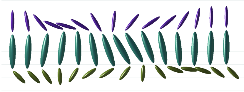
(a) Snapshots at each $0.7$ second

   

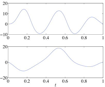
(b) Velocity of the central body (first and second component ($\mathrm{m/s}$))

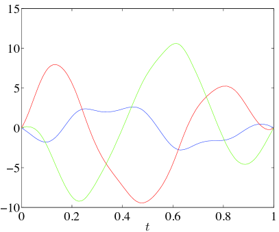
(c) Angular velocity (third components, red:$\Omega_{1}$, blue:$\Omega_{0}$, green:$\Omega_{2}$, ($\mathrm{rad/s}$))

(d) Linear momentum along the $e_{1}$ axis (dashed:rigid bodies, dotted:fluid, solid:total ($\mathrm{kgm/s}$))

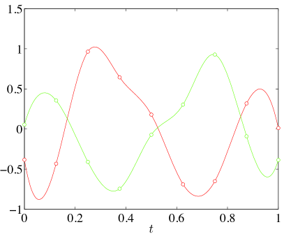
(e) Control moment (third components, red:$u_{1}$, green:$u_{2}$, ($\mathrm{kNm}$))

Figure 2: Optimal forward translation

Fig. 2 shows the optimal forward translation maneuver (an animation illustrating this maneuver is available at http://my.fit.edu/~taeyoung). The linear momentum exchange between rigid bodies and fluid along the $e_{1}$ axis is illustrated at Fig. 2(d). While the zero value of the total linear momentum is preserved throughout the maneuver, the average value of the linear momentum of the rigid bodies is positive. Therefore, the system of connected rigid bodies moves forward.

Fig. 3 illustrates the optimal rotation maneuver. It is interesting to observe that the optimal velocity, angular velocity, and control inputs are almost symmetric about the mid-maneuver time $t=0.5$. Similar to the optimal translation maneuver, at Fig. 3(d), the total angular momentum is preserved, but the average angular momentum of the rigid bodies about the rotation axis is positive. In addition to the angular momentum exchange between the rigid bodies and the fluid, this rotational maneuver is achieved by the geometric phase effect for coupled rigid bodies [18].

V Conclusion

For both cases, the proposed computational geometric optimal control approach successfully finds nontrivial optimal maneuvers of connected rigid bodies in a perfect fluid. These optimal maneuvers are based on the nonlinear coupling between the shape space and the group motions, and they involve large-angle rotations of connected rigid bodies.

The computational framework described in this paper extends the class of computationally tractable shape-based fish locomotion models to include three-dimensional articulated multibody systems, thereby allowing for the study of optimal shape maneuvers for fish movement patterns beyond that of carangiform locomotion.

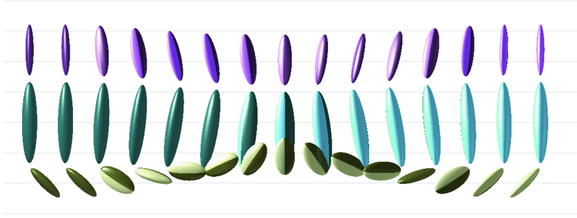
(a) Snapshots at each $0.7$ second (top view and back view)

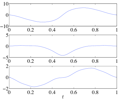
(b) Velocity of the central body (each component ($\mathrm{m/s}$))

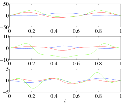
(c) Angular velocity (each component, red:$\Omega_{1}$, blue:$\Omega_{0}$, green:$\Omega_{2}$, ($\mathrm{rad/s}$))

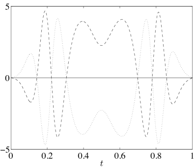
(d) Angular momentum about the $e_{1}$ axis (dahsed:rigid bodies, dotted:fluid, solid:total ($\mathrm{kgm/s}$))

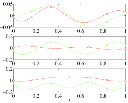
(e) Control moment (each component, red:$u_{1}$, green:$u_{2}$, ($\mathrm{kNm}$))

Figure 3: Optimal $180^{\circ}$ rotation about the $e_{1}$ axis

References

- [1] M. Sfakiotakis, D. Lane, and J. Davies, “Review of fish swimming modes for aquatic locomotion,” IEEE Journal of Oceanic Engineering, vol. 24, no. 2, pp. 237–252, 1999.
- [2] D. Barrett, “Propulsive efficiency of a flexible hull underwater vehicle,” Ph.D. dissertation, Massachusetts Institute of Technology, 1996.
- [3] E. Kanso, J. Marsden, C. Rowley, and J. Melli-Huber, “Locomotion of articulated bodies in a perfect fluid,” Journal of Nonlinear Science, vol. 15, pp. 255–289, 2005.
- [4] T. Lee, M. Leok, and N. H. McClamroch, “Dynamics of connected rigid bodies in a perfect fluid,” in Proceedings of the American Control Conference, 2009, pp. 408–413. [Online]. Available: http://arxiv.org/abs/0809.1488
- [5] T. Lee, “Computational geometric mechanics and control of rigid bodies,” Ph.D. dissertation, University of Michigan, 2008.
- [6] T. Lee, M. Leok, and N. H. McClamroch, “Lie group variational integrators for the full body problem in orbital mechanics,” Celestial Mechanics and Dynamical Astronomy, vol. 98, no. 2, pp. 121–144, June 2007.
- [7] J. Marsden, Lectures on Mechanics, ser. London Mathematical Society Lecture Note Series 174. Cambridge University Press, 1992.
- [8] T. Lee, M. Leok, and N. H. McClamroch, “Computational geometric optimal control of rigid bodies,” Communications in Information and Systems, special issue dedicated to R. W. Brockett, vol. 8, no. 4, pp. 445–472, 2008. [Online]. Available: http://arxiv.org/abs/0805.0639
- [9] E. Kanso and J. Marsden, “Optimal motion of an articulated body in a perfect fluid,” in Proceedings of the IEEE Conference on Decision and Control, 2005, pp. 2511–2516.
- [10] S. Ross, “Optimal flapping strokes for self-propulsion in a perfect fluid,” in Proceedings of the American Control Conference, 2006, pp. 4118–4122.
- [11] P. Holmes, J. Jenkins, and N. Leonard, “Dynamics of the Kirchhoff equations I: Coincident centers of gravity and bouyancy,” Physica D, vol. 118, pp. 311–342, 1998.
- [12] J. Marsden and T. Ratiu, Introduction to Mechanics and Symmetry, 2nd ed., ser. Texts in Applied Mathematics. Springer-Verlag, 1999, vol. 17.
- [13] E. Hairer, C. Lubich, and G. Wanner, Geometric Numerical Integration, 2nd ed., ser. Springer Series in Computational Mathematics. Springer-Verlag, 2006, vol. 31.
- [14] J. Marsden and M. West, “Discrete mechanics and variational integrators,” in Acta Numerica. Cambridge University Press, 2001, vol. 10, pp. 317–514.
- [15] M. Reyhanoglu and N. H. McClamroch, “Reorientation maneuvers of planar multibody systems in space using internal controls,” AIAA Journal of Guidance, Control and Dynamics, vol. 15, no. 6, pp. 1475–1480, 1992.
- [16] C. Rui, I. Kolmanovsky, and N. H. McClamroch, “Nonlinear attitude and shape control of spacecraft with articulated appendages and reaction wheels,” IEEE Transactions on Automatic Control, vol. 45, no. 8, pp. 1455–1469, 2000.
- [17] T. Lee, M. Leok, and N. H. McClamroch, “Optimal attitude control for a rigid body with symmetry,” in Proceedings of the American Control Conference, 2007, pp. 1073–1078. [Online]. Available: http://arxiv.org/abs/math.OC/06009482
- [18] R. Montgomery, “Guage theory of the falling cat,” in Dynamics and control of mechanical systems: the falling cat and related problems, ser. Fields Institute Communications, M. Enos, Ed. American Mathematical Society, 1991, pp. 193–218.