Quantum Yang-Mills Condensate Dark Energy Models

Abstract

We review the quantum Yang-Mills condensate (YMC) dark energy models. As the effective Yang-Mills Lagrangian is completely determined by the quantum field theory, there is no adjustable parameter in the model except the energy scale. In this model, the equation-of-state (EOS) of the YMC dark energy, $w_{y}>-1$ and $w_{y}<-1$, can both be naturally realized. By studying the evolution of various components in the model, we find that, in the early stage of the universe, dark energy tracked the evolution of the radiation, i.e. $w_{y}\rightarrow 1/3$. However, in the late stage, $w_{y}$ naturally runs to the critical state with $w_{y}=-1$, and the universe transits from matter-dominated into dark energy dominated stage only at recently $z\sim 0.3$. These characters are independent of the choice of the initial condition, and the cosmic coincidence problem is avoided in the models. We also find that, if the possible interaction between YMC and dust matter is considered, the late time attractor solution may exist. In this case, the EOS of YMC must evolve from $w_{y}>0$ into $w_{y}<-1$, which is slightly suggested by the observations. At the same time, the total EOS in the attractor solution is $w_{tot}=-1$, the universe being the de Sitter expansion in the late stage, and the cosmic big rip is naturally avoided. These features are all independent of the interacting forms.

I Introduction

The observations of Type Ia Supernova (SNIa) sn , together with the cosmic microwave background radiation (CMB)map and the larger scale structure sdss , suggest that the present universe is accelerating expansion, which needs a kind of mysterious dark energy with negative equation-of-state (EOS). The simplest model is by introducing the cosmological constant term $\Lambda$, which has a constant effective EOS $w=-1$, and drive the acceleration of the universe. If assuming the effective energy of the $\Lambda$ term occupies $\sim 73\%$ of the total energy, together with $\sim 23\%$ dark matter, $\sim 4\%$ baryon matter and $\sim 10^{-5}$ radiation component, constitute the so-called $\Lambda$CDM model.

Although this simple model satisfies nearly all the cosmological observations, it still remains a phenomenological model. Since the major components, $\Lambda$ and dark matter, still keep unclear for us. For the $\Lambda$ as the candidate of dark energy, also suffers from the following dilemmas (see for instant constant ): First, the effective energy density is quite tiny, $\rho_{\Lambda}\sim 5.8h^{2}\times 10^{-11}$eV⁴. If we consider it as the vacuum energy of the particle physics, this energy density is $120$ order smaller than the Planck energy scale! This is the so-called ‘fine-tunning’ problem. Second, the density scale of $\Lambda$ keeps constant in all the stage of the universe. The observations show that the present value of the matter component (including dark matter and baryon components) is some one third of $\rho_{\Lambda}$, but it varies with time as $\rho_{m}\propto a^{-3}$. So, for example, at an earlier time of radiation-matter equality with redshift $z\sim 3454$, $\rho_{\Lambda}$ should be a very fine tuned value $\sim 6.3\times 10^{-11}\rho_{m}$. Otherwise, a slightly variant initial value of $\rho_{\Lambda}$ would lead to a value of the ratio $\rho_{\Lambda}/\rho_{m}$ drastically different from the observed one. This is the so-called ‘coincidence’ problem. In addition, the $\Lambda$CDM model also faces some observational challenges: there are mild evidences show that, the EOS of dark energy might evolve from $w>-1$ in the early stage to $w<-1$ in the current stage cross2 , which is expected to be confirmed by the future sensitive observations detf .

So, it is necessary to look for other candidates as the dark energy, especially the dynamical models. One possibility is proposing a canonical scalar field $\phi$ with the langrangian $\mathcal{L}_{\phi}=\dot{\phi}^{2}/2-V(\phi)$, which is dubbed as the ‘quintessence’ models (see the review scalarreview ). Similar to the inflationary field, when the potential term $V(\phi)$ is dominant, the EOS of the quintessence field approaches to $-1$, i.e. $\Lambda$-like, and accounts for the observations. The most interesting is that, in track-quint , the authors introduced a kind of potential forms, such as $V(\phi)=M^{4+\alpha}\phi^{-\alpha}$ or $V(\phi)=M^{4}[\exp(M_{\rm pl}/\phi)-1]$, which have the tracker solutions, i.e. the field $\phi$ tracked the evolution of the background components in the early universe. So they address the coincidence problem, i.e. removing the need to tune initial conditions in order for the matter and dark energy densities to nearly coincide today. Although, this kind of models have been excluded by the cosmological observations, it provides the excellent possibility to naturally avoided the coincidence problems.

However, the quintessence models also suffer from some dilemmas. The EOS of the quintessence models are in the range $-1<w<1$. In order to obtain a EOS with $w<-1$, one always has to introduce the so-called ‘phantom’ field, which includes the non-canonical negative kinetic terms phantom quintom . However, the ‘phantom’ field lacks the strong physical motivation, and also leads to the problem of quantum instabilities stable . In bigrip , the authors also pointed that, if $w<-1$ keeps, the universe shall face the ‘big-rip’ problem.

In addition to proposing the dynamical dark energy models, some efforts have been paid to modify the general relativity (GR) gravity , which can also speed-up the universe in the recent stage. However, it should be pointed that, any revised GR should prepare to go through the strict solar system test solar , as well as to explain the various cosmological observations, such as the CMB temperature and polarization anisotropies power spectra. In addition, to our view, the current observations have not provided the strong reasons to answer: Why we should modify GR and how to modify it.

In this paper, we shall propose the Yang-Mills condensate (YMC) dark energy models, where, instead of the scalar field, the quantum Yang-Mills field is considered as the candidate of dark energy component. Recently, the similar models are also discussed by a number of authors vector emfield . Different from the scalar field models, the Yang-Mills fields are the indispensable cornerstone to particle physics, gauge bosons have been observed. There is no room for adjusting the form of effective Yang-Mills Lagrangian as it is predicted by quantum corrections according to field theory. In this review, we shall firstly introduce physical motivations of the YMC dark energy models in Section II. In Section III, we simply introduce and discuss the Lagrangian of effective quantum Yang-Mills field.

As the main part of this paper, in Section IV, we apply the YMC into the cosmology as the candidate of dark energy, and investigate the cosmic evolution of the various components, especially the evolution of dark energy. We find the excellent characters of this kind of models. Different from the quintessence models, both the EOS $w_{y}>-1$ and $w_{y}<-1$ can be naturally realized. In the free YMC dark energy models, $w_{y}\rightarrow 1/3$ in the early stage and tracked the evolution of radiation component. Only in the recent stage, $w_{y}$ rolls to the critical state with $w_{y}=-1$, i.e. $\Lambda$-like, and accounts for the observations. This feature is independent of the choice of the initial condition, so the coincidence problem is naturally avoided. We also find that, if the possible interaction between YMC and dust components is considered, the late time attractor solution can exist, where the EOS of YMC naturally runs from $w_{y}\rightarrow 1/3$ to the the phantom-like attractor state, i.e. $w_{y}<-1$. However, the total effective EOS is $w_{tot}=-1$ in the attractor solution, and the so-called ‘big-rip’ problem is also avoided. We should pointed that, these new features are all independent of the interaction forms. In Section V, we calculate the statefinder and $Om$diagnostics for the YMC dark energy models, which are helpful to differentiate the YMC models from the other dark energy models from the observations.

Section VI is contributed as a summary of this paper.

Throughout this paper, we will work with unit in which $c=\hbar=k_{B}=1$.

II physical motivation

The introduction of the quantum effective YMC into cosmology y has been motivated by the fact that the $SU(3)$ YMC has given a phenomenological description of the vacuum within hadrons confining quarks, and yet at the same time all the important properties of a proper quantum field are kept, such as the Lorentz invariance, the gauge symmetry, and the correct trace anomaly 23 25 . Quarks inside a hadron would experience the existence of the Bag constant, $B$, which is equivalent to an energy density $B$ and a pressure $-B$. So quarks would feel an energy-momentum tensor of the vacuum as $T_{\mu\nu}=B{\rm diag}(1,-1,-1,-1)$. This non-trivial vacuum has been formed mainly by the contributions from the quantum effective YMC, and from the possible interactions with quarks. Our thinking has been that if the vacuum inside a hadron is filled with the quantum effective YMC, what if the vacuum of the universe as a whole is also filled with some kind of YMC.

Gauge fields play a very important role in, and are the indispensable cornerstone to, particle physics. All known fundamental interactions between particles are mediated through gauge bosons. Generally speaking, as a gauge field, the YMC under consideration may have interactions with other species of particles in the universe. However, unlike those well known interactions in QED, QCD, and the electro-weak unification, here at the moment we do not yet have a model for the details of the microscopic interactions between the YMC and other particle. Therefore, in this paper on the dark energy model based on the quantum effective YMC, we will adopt a simple description of the possible interactions between the YMC and other cosmic particles, in addition to the simplest model with free YMC component. We will investigate in these models the cosmic evolution of the universe from the radiation-dominated era up to the present.

III Yang-Mills field model

In the effective YMC dark energy model, the effective Yang-Mills field Lagrangian is given by 23 zzcqg2006 ; zzplb2006 :

$$\mathcal{L}_{\rm eff}=\frac{1}{2}bF\left(\ln\left|{F}/{\kappa^{2}}\right|-1\right),$$ (1)

where $\kappa$ is the renormalization scale of dimension of squared mass, $F\equiv-(1/2)F^{a}_{\mu\nu}F^{a\mu\nu}$ plays the role of the order parameter of the YMC. The Callan-Symanzik coefficient $b=(11N-2N_{f})/24\pi^{2}$ for $SU(N)$ with $N_{f}$ being the number of quark flavors. For the gauge group $SU(2)$ considered here, one has $b=11/12\pi^{2}$ when the fermion’s contribution is neglected. For the case of $SU(3)$ the effective Lagrangian in (1) leads to a phenomenological description of the asymptotic freedom for quarks inside hadrons 23 . It should be noted that the $SU(2)$ Yang-Mills field is introduced here as a model for the cosmic dark energy, in may not be directly identified as the QCD fields, nor the weak-electromagnetic unification gauge fields.

An explanation can be given for the form in (1) as an effective Lagrangian up to 1-loop quantum correct 23 ; 24 ; 25 . A classical $SU(N)$ Yang-Mills field Lagrangian is $\mathcal{L}=F/2g_{0}^{2}$, where $g_{0}$ is the bare coupling constant. As is known. when 1-loop quantum corrections are included, the bare coupling $g_{0}$ will be replaced by a running one $g$ as the following 26 , $g_{0}^{2}\rightarrow g^{2}=2/(b\ln(k^{2}/k_{0}^{2}))$, where $k$ is the momentum transfer and $k_{0}$ is the energy scale. To build up an effective theory 23 ; 24 ; 25 , one may just replace the momentum transfer $k^{2}$ by the field strength $F$ in the following manner: $\ln(k^{2}/k_{0}^{2})\rightarrow 2\ln|F/e\kappa^{2}|$, yielding equation (1). We would like to point out that the renormalization scale $\kappa$ is the only parameter of this effective Yang-Mills model, and its value should be determined by comparing the observations. In contrast to the scalar field dark energy models, the YMC Lagrangian is completely fixed by quantum corrections up to 1-loops, and there is no room for adjusting its functional form. This is an attractive feature of the effective YMC dark energy model. We should mention that, the YMC dark energy models including 2-loop and 3-loop quantum corrects are also discussed in the recent papers xzplb2007 wzxjcap2008 . It was found that, these more complicated models have the exactly same characters with the 1-loop models. So in this paper, we mainly focus on the 1-loop models with the Lagrangian in (1).

IV YMC as dark energy

Let us work in the flat Friedmann-Lemaitre-Robertson-Walker (FLRW) universe, which is described by

$$ds^{2}=dt^{2}-a^{2}(t)\delta_{ij}dx^{i}dx^{j}=a^{2}(\tau)[d\tau^{2}-\delta_{ij}dx^{i}dx^{j}],$$

where $t$ time and $\tau$ time are related by $cdt=ad\tau$. Considering the simplest case with only the YMC in the universe, which minimally coupled to the gravity, the effective action is,

$$S=\int\sqrt{-{g}}~{}\left[-\frac{\mathcal{R}}{16\pi G}+\mathcal{L}_{\rm eff}\right]~{}d^{4}x.$$ (2)

Here, ${g}$ is the determinant of the metric $g_{\mu\nu}$. $\mathcal{R}$ is the scalar Ricci curvature, and $\mathcal{L}_{\rm eff}$ is the effective Lagrangian of YMC, described by Eq. (1). By variation of $S$ with respect to the metric $g^{\mu\nu}$, one obtains the Einstein equation $G_{\mu\nu}=8\pi GT_{\mu\nu}$, where the energy-momentum tensor of YMC is given by

$$T_{\mu\nu}=\sum_{a=1}^{3}~{}\frac{g_{\mu\nu}}{4g^{2}}F_{\sigma\delta}^{a}F^{a\sigma\delta}+\epsilon F_{\mu\sigma}^{a}F^{a\sigma}_{\nu}.$$ (3)

The dielectric constant is defined by $\epsilon\equiv 2\partial\mathcal{L}_{\rm eff}/\partial F$. In the one-loop order, it is given by

$$\epsilon=b\ln\left|{F}/{\kappa^{2}}\right|.$$ (4)

This energy-momentum tensor (3) is the sum of three different energy-momentum tensors of the vectors, $T_{\mu\nu}=\sum_{a}~{}^{(a)}T_{\mu\nu}$, neither of which is of prefect-fluid form. Here we assume the gauge fields are only the functions of time $t$, and $A_{\mu}=\frac{i}{2}\sigma_{a}A_{\mu}^{a}(t)$ (here $\sigma_{a}$ are the Pauli’s matrices) are given by $A_{0}=0$ and $A_{i}^{a}=\delta_{i}^{a}A(t)$. Thus, we will find that, the total energy-momentum tensor $T_{\mu\nu}$ is homogeneous and isotropic.

Define the Yang-Mills field tensor as usual:

$$F^{a}_{\mu\nu}=\partial_{\mu}A_{\nu}^{a}-\partial_{\nu}A_{\mu}^{a}+f^{abc}A_{\mu}^{b}A_{\nu}^{c},$$ (5)

where $f^{abc}$ is the structure constant of gauge group and $f^{abc}=\epsilon^{abc}$ for the $SU(2)$ case. This tensor can be written in the form with the electric and magnetic field as

$$F^{a\mu}_{~{}~{}\nu}=\left(\begin{array}[]{cccc}0&E_{1}&E_{2}&E_{3}\\ -E_{1}&0&B_{3}&-B_{2}\\ -E_{2}&-B_{3}&0&B_{1}\\ -E_{3}&B_{2}&-B_{1}&0\end{array}\right).$$ (10)

It can be easily found that $E_{1}^{2}=E_{2}^{2}=E_{3}^{2}$, and $B_{1}^{2}=B_{2}^{2}=B_{3}^{2}$. Thus $F$ has a simple form with $F=E^{2}-B^{2}$, where $E^{2}=\sum_{i=1}^{3}E_{i}^{2}$ and $B^{2}=\sum_{i=1}^{3}B_{i}^{2}$. In this case, each component of the energy-momentum tensor is

$${}^{(a)}T_{\mu}^{0} = \frac{1}{6}(\epsilon-b)(B^{2}-E^{2})\delta^{0}_{\mu}+\frac{\epsilon}{3}E^{2}\delta^{0}_{\mu},$$ (11)

$${}^{(a)}T_{j}^{i} = \frac{1}{6}(\epsilon-b)(B^{2}-E^{2})\delta^{i}_{j}+\frac{\epsilon}{3}E^{2}\delta^{i}_{j}\delta^{a}_{j}-\frac{\epsilon}{3}B^{2}\delta^{i}_{j}(1-\delta^{a}_{j}).$$ (12)

Although this tensor is not isotropic, its value along the $j=a$ direction is different from the ones along the directions perpendicular to it. However, the total energy-momentum tensor $T_{\mu\nu}=\sum_{a=1}^{3}~{}^{(a)}T_{\mu\nu}$ has isotropic stresses, and the corresponding energy density and pressure are given by

$$\rho_{y}=\frac{1}{2}\epsilon(E^{2}+B^{2})+\frac{1}{2}b(E^{2}-B^{2}),~{}~{}p_{y}=\frac{1}{6}\epsilon(E^{2}+B^{2})-\frac{1}{2}b(E^{2}-B^{2}).$$ (13)

In this paper, for simplicity, we only discuss the pure ‘electric’ case, $F=E^{2}$. This is a typical consideration, since in the expanding universe, a given ‘magnetic’ component of Yang-Mills field decreases quite rapidly, and the Yang-Mills field becomes the ‘electric’ type zxijmpd2007 . The energy density and pressure of YMC are reduced to

$$\rho_{y}=\frac{E^{2}}{2}(\epsilon+b),~{}~{}p_{y}=\frac{E^{2}}{2}\left(\frac{\epsilon}{3}-b\right).$$

It is convenient to introduce a dimensionless quantity $y\equiv\epsilon/b=\ln|F/\kappa^{2}|$. So the quantities $\rho_{y}$ and $p_{y}$ can be rewritten as

$$\rho_{y}=\frac{1}{2}b\kappa^{2}(y+1)e^{y},~{}~{}p_{y}=\frac{1}{6}b\kappa^{2}(y-3)e^{y}.$$ (14)

One sees that, to ensure that energy density $\rho_{y}$ be positive in any physically viable model, the allowance for the quantity $y$ should be $y>-1$, i.e. $F>\kappa^{2}/e\simeq 0.368\kappa^{2}$. The EOS of the YMC is

$$w_{y}\equiv\frac{p_{y}}{\rho_{y}}=\frac{y-3}{3y+3}.$$ (15)

Before setting up a cosmological model, the EOS $w_{y}$ itself as a function of $F$ is interesting. At the state with $F=\kappa^{2}$, which is called critical point, one has $y=0$ and the YMC has an EOS of the cosmological constant with $w_{y}=-1$. Around this critical point, $F<\kappa^{2}$ gives $y<0$ and $w<-1$, and $F>\kappa^{2}$ gives $y>0$ and $w>-1$. So in the YMC dark energy models, EOS with $w>-1$ and $w<-1$ all can be naturally realized. On the other hand, in the high energy scale with $F\gg\kappa^{2}$, one finds that the YMC exhibits an EOS of radiation with $w_{y}=1/3$. In the follows, we will detailed show that the YMC was evolving from the state with $w_{y}=1/3$ to $w_{y}=-1$ (or even to $w_{y}<-1$) in the expanding universe. This is the main context in this paper. In addition, the characteristic statefinder parameters and the perturbations of the YMC dark energy is also discussed in zijmpd2008 ; tzxijmpd2009 zraa2009 , which are helpful to distinguish the YMC model from other dark energy models.

As is known, an effective theory is a simple representation for an interacting quantum system of many degrees of freedom at and around its respective low energies. Commonly, it applies only in low energies. However, it is interesting to note that the YMC model as an effective theory intrinsically incorporates the appropriate states for both high and low temperature. As has been shown, the same expression in (15) simultaneously gives $p_{y}\sim-\rho_{y}$ at low energies, and $p_{y}\rightarrow\rho_{y}/3$ at high energies. Therefore, the model of effective YMC can be used even at higher energies than the renormalization scale $\kappa$.

IV.1 Free YMC models

Let us discuss the cosmological model, which filled with three kinds of major energy components, the dark energy, the matter, including both baryons and dark matter, and the radiation. Here, the dark energy component is represented by YMC, and the matter component is simply described by a non-relativistic dust with negligible pressure, and the radiation component consists of the photons and possibly other particles, such as the neutrino, if they are massless.

Since the universe is assumed to be flat, the sum of the fraction densities is $\Omega_{y}+\Omega_{m}+\Omega_{r}=1$, where the fractional energy densities are $\Omega_{y}\equiv\rho_{y}/\rho_{tot}$, $\Omega_{m}\equiv\rho_{m}/\rho_{tot}$, $\Omega_{r}\equiv\rho_{r}/\rho_{tot}$, and the total energy density is $\rho_{tot}\equiv\rho_{y}+\rho_{m}+\rho_{r}$. The overall expansion of the universe is determined by the Friedmann equations:

$$\left(\frac{\dot{a}}{a}\right)^{2}=\frac{8\pi G}{3}(\rho_{y}+\rho_{m}+\rho_{r}),$$ (16)

$$\frac{\ddot{a}}{a}=-\frac{4\pi G}{3}(\rho_{y}+3p_{y}+\rho_{m}+\rho_{r}+3\rho_{r}),$$ (17)

where and what follows, the superscript $dot$ denote the $d/dt$. These three components of energy contribute to the source on the right-hand side of the equations. We should notice that, $p_{r}=\rho_{r}/3$. In this subsection, we shall assume there is no interaction between these three components. The dynamical evolutions of the three components are determined by their equations of motion, which can be written as equations of the conservation of energy,

$$\dot{\rho}_{y}+3\frac{\dot{a}}{a}(\rho_{y}+p_{y})=0,$$ (18)

$$\dot{\rho}_{m}+3\frac{\dot{a}}{a}\rho_{m}=0,$$ (19)

$$\dot{\rho}_{r}+3\frac{\dot{a}}{a}(\rho_{r}+p_{r})=0.$$ (20)

As is known, Eq. (17) is not independent and can be derived from Eqs. (18), (19), (20) and (16). From Eqs. (19) and (20), we can obtain the evolutions of the matter and radiation components, $\rho_{m}\propto a^{-3}$ and $\rho_{m}\propto a^{-4}$.

Now, let us focus on the evolution of YMC. Inserting (14) into (18), we can obtain the following simple relation,

$$ye^{y/2}\propto a^{-2},$$ (21)

where the coefficient of proportionality in the above depends on the initial condition. At the early stages, $a\rightarrow 0$, Eq. (21) leads to $y\gg 1$, and Eq. (15) gives $w_{y}\rightarrow 1/3$, so the YMC behaves as the radiation component. With the expansion of the universe, the value of $y$ runs to the critical state of $y=0$, and the EOS goes to $w_{y}=-1$. So, in the late stage of the universe, the YMC behaves as the cosmological constant. This is one of the most attractive character of the YMC models. Around the critical point with $y=0$, Eq.(21) yields $y\propto a^{-2}$, and the EOS of YMC is $w_{y}+1\simeq{4y}/{3}\propto a^{-2}$. The YMC can achieve the states of $w_{y}>-1$ and $w_{y}<-1$, but it can not cross over $-1$, just like in the scalar models cross .

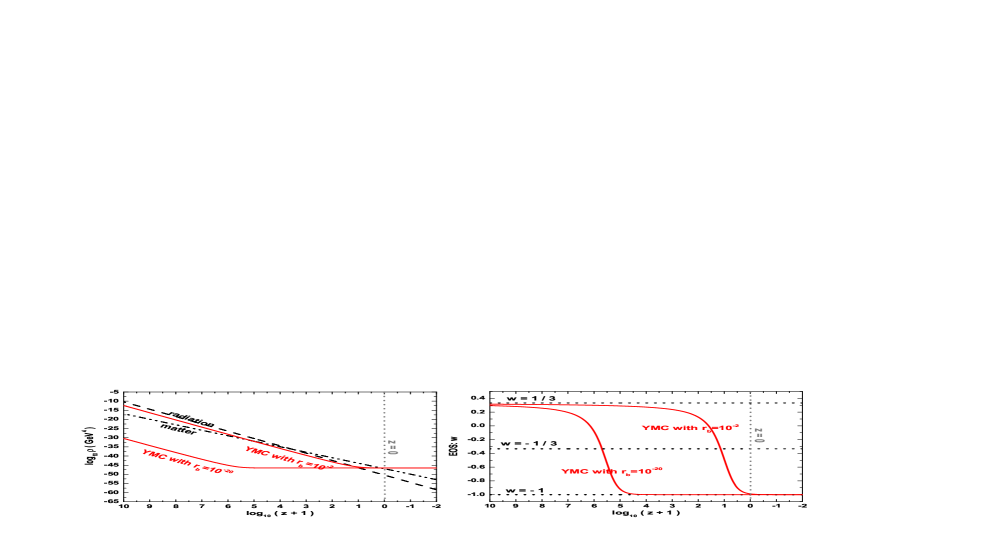
Figure 1: In the free YMC dark energy models, the evolution of the YMC energy density (left panels) and EOS (right panels) for the models with different initial conditions.

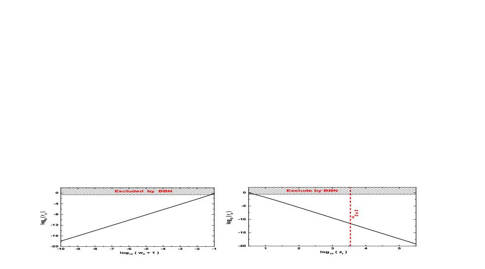
Figure 2: Left panel: The present EOS of the YMC $w_{0}$ depends on the initial value $r_{b}$. Right panel: The transition redshift $z_{t}$ depends on the initial value $r_{b}$. In both panels, the shadow region has been excluded by the observation of BBN.

We should notice that, the relation in (21) can also be derived by the effective Yang-Mills equations. By variation of the action $S$ with respect to gauge field $A_{\mu}^{a}$, we can obtain the Yang-Mills equations, which are

$$\partial_{\mu}(a^{4}\epsilon~{}F^{a\mu\nu})+f^{abc}A_{\mu}^{b}(a^{4}\epsilon~{}F^{c\mu\nu})=0.$$ (22)

The $\nu=0$ component of which is an identity, and the $\nu=1,2,3$ spatial components can be reduced to $\partial_{\tau}(a^{2}\epsilon E)=0$. At the critical point ($\epsilon=0$), this equation is an identity. When $\epsilon\neq 0$, this equation has an exact solution as (21) zzplb2006 .

Now, let us fix the value of $\kappa$, the only parameter in the model. At the present time, the YMC energy density is

$$\rho_{y}=\frac{bE^{2}}{2}(y+1)\simeq\frac{b\kappa^{2}}{2},$$ (23)

and, as the dark energy, it should be $\Omega_{y}\rho_{tot}$, where the present total energy density in the universe $\rho_{tot}\approx 8.099\,h^{2}\times 10^{-11}\rm{eV}^{4}$. We choose $\Omega_{y}=0.73$ as has been observed, yielding

$$\kappa=3.57\,h\times 10^{-5}{\rm eV}^{2}.$$ (24)

This energy scale is low compared to typical energy scales in particle physics, such as the QCD and the weak-electromagnetic unification. This is the reason, why the $SU(2)$ Yang-Millls field introduced in this paper cannot be directly identified as the the QCD gluon fields, nor the weak-electromagnetic unification gauge fields.

To be more specific about how the YMC evolves in the expanding universe, we look at an early stage when the Big Bang nucleosynthesis (BBN) processes occur around a redshift $z\sim 10^{10}$ with an energy scale $\sim 1$MeV. To see how the evolution of $\rho_{y}$ depends the the initial condition, we introduce the ratio of energies of the two components

$$r_{b}\equiv\left.\frac{\rho_{y}}{\rho_{r}}\right|_{z=10^{10}},$$ (25)

where $\rho_{r}$ is the radiation energy density. We consider $r_{b}<1$, i.e. the YMC is subdominant to the radiation component initially. Of course, the YMC evolves differently for different initial values of $r_{b}$. Nevertheless, we will see that, as the result of evolution, the present universe is always dominated by the YMC $\Omega_{y}\sim 0.73$ for a very wide range of initial values $r_{b}$.

Now we use the exact solution (21) to plot the evolution of $\rho_{y}$ as a function of the redshift $z$ in Fig. 1 (left panel). As specific examples, here we take $r_{b}=10^{-2}$, and $r_{b}=10^{-20}$. In comparison, also plotted are the energy densities of radiation, and of matter. It is seen that, in the early stages, $\rho_{y}$ decreases as $\rho_{y}\propto a^{-4}$. So the YMC density is subdominant and tracks the radiation, a scaling solution. The corresponding EOS of Yang-Mills field is $w_{y}\simeq 1/3$ shown in Fig. 1 (right panel). At late stages, with the expansion of the universe, $a\rightarrow\infty$, $y$ decreases to nearly zero, and $w_{y}\rightarrow-1$ asymptotically. Moreover, this asymptotic region is arrived at some redshift $z$ before the present time, and this $z$ has different values for different initial values of $r_{b}$. For smaller $r_{b}$, the transition redshift is larger (seen in Fig. 1), and the transition happens earlier. Once the asymptotic region is achieved, the density of the YMC levels off and remain a constant forever, like a cosmological constant. We have also checked that the present value $\Omega_{y}\sim 0.73$ is also the outcome of the cosmic evolution for any value of $r_{b}$ in the very wide range $(10^{-20},10^{-2})$. So the coincidence problem do not exist in the YMC model.

The present EOS of the YMC $w_{0}$ is nearly $-1$. Fig. 2 (left panel) plots the dependence of the present EOS $w_{0}$ on the initial condition $r_{b}$. The function $\log_{10}(r_{b})$ versus $\log_{10}(w_{0}+1)$ is nearly linear: a smaller $r_{b}$ leads to a smaller $w_{0}$. For a value $r_{b}=10^{-2}$, one has $w_{0}=-0.99$. For a value $r_{b}=10^{-20}$, $w_{0}$ would be $-1$ accurately up to one in $10^{11}$. Therefore, at present the YMC is very similar to the cosmological constant.

The solution in Eq.(21) can converted into the following form

$$z=\sqrt{\frac{y}{y_{0}}}\exp\left[\frac{y-y_{0}}{4}\right]-1,$$ (26)

where $y_{0}$ is the value of $y$ at $z=0$, depending on the initial value $r_{b}$. For a fixed $y_{0}$, this formula tells a one-one relation between the EOS (through $y$) and the corresponding redshift $z$. As is seen from Fig. 1, the transition of $\omega$ from $1/3$ to $-1$ occurs during a finite period of time, instead of instantly. To characterize the time of transition, we use $z_{t}$ to denote the redshift when $\omega=-1/3$, i.e. $y=1$, as given by Eq.(15). This is, in fact, the time when the strong energy condition begins to be violated, i.e., $\rho_{y}+3p_{y}\leq 0$. Then

$$z_{t}=\sqrt{\frac{1}{y_{0}}}\exp\left[\frac{1-y_{0}}{4}\right]-1.$$ (27)

Therefore, this gives a function $z_{t}=z_{t}(r_{b})$. Fig. 2 (right panel) shows how the transition redshift $z_{t}$ depends on the ratio $r_{b}$. Interestingly, this transition can occur before, or after the radiation-matter equality ($z_{eq}=3454$). This feature is different from the tracked quintessence models in which transition occurs during the matter dominated era track-quint . A larger $r_{b}$ leads to a smaller $z_{t}$. For example, $r_{b}=10^{-2}$ leads to $z_{t}\simeq 12.4\ll z_{eq}$, and the transition occurs in the matter dominated stage, and $r_{b}=10^{-20}$ leads to $z_{t}\simeq 5.0\times 10^{5}\gg z_{eq}$, and the transition occurs in the radiation dominated stage.

The value of $r_{b}$ cannot be chosen to arbitrarily large. In fact, there is a constraint from the observation result of the BBN. As is known, the presence of dark energy during nucleosynthesis epoch will speedup the expansion, enhancing the effective species $N_{\nu}$ of neutrinos bbn . The latest analysis gives a constrain on the extra neutrino species $\delta N_{\nu}\equiv N_{\nu}-3<1.60$ bbn . Here in our model, the dark energy is played by the YM field. By a similar analysis, the ratio $r_{b}$ is related to $\delta N_{\nu}$ through $r_{b}=\frac{7\delta N_{\nu}/4}{10.75}$. This leads to an upper limit $r_{b}<0.26$, the present EoS $w_{0}<-0.94$ by Fig. 2 (left panel), and the transition redshift $z_{t}>5.8$ by Fig. 2 (right panel). The range of initial conditions $r_{b}\in(10^{-20},10^{-2})$ that we have taken satisfies this constraint.

IV.2 Coupled YMC models

In this subsection, we shall generalize the original YMC dark energy model to include the interaction between the YMC and dust matter. We should mention that, the possible interaction between YMC and radiation component may also exist, which has been discussed in xzzcqg2007 . (The similar models on the scalar field dark energy have been discussed by a number of authors (see wangbing for instant)). In this section, we assume the YMC dark energy and background matter interact through an interaction term $Q$. Thus the equations of the conservation of energy in (18) and (19) should be changed into

$$\dot{\rho}_{y}+3\frac{\dot{a}}{a}(\rho_{y}+p_{y})=-Q,$$ (28)

$$\dot{\rho}_{m}+3\frac{\dot{a}}{a}\rho_{m}=Q,$$ (29)

and the equation for radiation in (20) is still held. The sum of Eqs. (28) and (29) guarantees that the total energy of YMC and dust matter is still conserved. It is worth noting that the free Yang-Mills equation in (22) is not satisfied when $Q\neq 0$. In the natural unit, the interaction term $Q$ has the dimension of $[{\rm energy}]^{5}$. The coupling $Q$ is phenomenological, and their specific forms will be addressed later. When $Q>0$, the YMC transfers energy into the matter, and this could be implemented, for instance, by the processes with the YMC decaying into pairs of matter particles. On the other hand, when $Q<0$, the matter transfers energy into the YMC. Note that, once $Q$ is introduced as above, it will bring another new parameters in the models, in addition the free parameter $\kappa$.

We introduce the following dimensionless variables, rescaled by the critical energy density $b\kappa^{2}/2$ of the YMC,

$$x\equiv\frac{2\rho_{m}}{b\kappa^{2}},~{}~{}f\equiv\frac{2Q}{b\kappa^{2}H},$$ (30)

where $f$ is the function of $x$ and $y$. By the help of the definition of $y$, the evolution equations (28) and (29) can be rewritten as a dynamical system, i.e.

$$y^{\prime} = -\frac{4y}{2+y}-\frac{f(x,y)}{(2+y)e^{y}},$$ (31)

$$x^{\prime} = -3x+f(x,y).$$ (32)

Here, a prime denotes derivative with respect to the so-called e-folding time $N\equiv\ln a$. The fractional energy densities of dark energy and background matter are given by

$$\Omega_{y}=\frac{(1+y)e^{y}}{(1+y)e^{y}+x},~{}~{}{\rm and}~{}~{}\Omega_{m}=\frac{x}{(1+y)e^{y}+x}.$$ (33)

Before discussing the specific form of the interaction term $Q$, let us first investigate the general feature of this dynamical system, described by (31) and (32). We can obtain the critical point $(y_{c},x_{c})$ of the autonomous system by imposing the conditions $y_{c}^{\prime}=x_{c}^{\prime}=0$. From the equations (31) and (32), we obtain that the critical state satisfies the following simple relations

$$3x_{c} = f(x_{c},y_{c}),$$ (34)

$$3x_{c} = -4y_{c}e^{y_{c}}.$$ (35)

So we can obtain the critical state $(y_{c},x_{c})$ by solving these two equations. In order to study the stability of the critical point, we substitute linear perturbations $y\rightarrow y_{c}+\delta y$ and $x\rightarrow x_{c}+\delta x$ about the critical point into dynamical system equations (31) and (32) and linearize them. Thus, two independent evolutive equations are derived,

$$\left(\begin{array}[]{c}\delta y^{\prime}\\ \delta x^{\prime}\end{array}\right)\equiv M\left(\begin{array}[]{c}\delta y\\ \delta x\end{array}\right)=\left(\begin{array}[]{cc}G_{,\rm y}+R_{,\rm y}&R_{,\rm x}\\ f_{,\rm y}&f_{,\rm x}-3\end{array}\right)\left(\begin{array}[]{c}\delta y\\ \delta x\end{array}\right),$$

where $R_{,\rm y}\equiv\partial R/\partial y$ at $(y,x)=(y_{c},x_{c})$. The definitions of $R_{,\rm x}$, $f_{,\rm y}$, $f_{,\rm x}$ and $G_{,\rm y}$ are similar. The functions $G$ and $R$ are defined by

$$G\equiv G(y)=-\frac{4y}{2+y},~{}~{}~{}R\equiv R(x,y)=-\frac{f(x,y)}{(2+y)e^{y}},$$

which are used for the simplification of the notation. The two eigenvalues of the coefficient matrix $M$ determine the stability of the corresponding critical point. The critical point is an attractor solution, which is stable, only if both the these two eigenvalues are negative (stable node), or real parts of these two eigenvalues are negative and the determinant of the matrix $M$ is negative (stable spiral).

Here we discuss some general features of the attractor solutions, regardless the special form of the interaction term $Q$. From the expression (35), we find that $x_{c}=-(4/3)y_{c}e^{y_{c}}$. Substitute this into the formula (33), one obtains

$$\Omega_{y}=\frac{(y_{c}+1)e^{y_{c}}}{(y_{c}+1)e^{y_{c}}+x_{c}}=\frac{3+3y_{c}}{3-y_{c}}.$$ (36)

Since $0\leq\Omega_{y}\leq 1$, this formula follows a constraint of the critical point

$$-1\leq y_{c}\leq 0.$$ (37)

From the formulae (15) and (36), we find a simple, but interesting relation,

$$\Omega_{y}w_{y}=-1.$$ (38)

This relation is held for all attractor solutions, independent of the special form of the interaction. Since the value of $\Omega_{y}$ is smaller than or equal to unity in the attractor solution, we obtain that

$$w_{y}\leq-1.$$ (39)

This means that, the EOS of the YMC dark energy must be smaller than or equal to $-1$, i.e. phantom-like or $\Lambda$-like. Since in the early universe, the value of the order parameter of the YM field $F$ is much larger than that of $\kappa^{2}$, i.e. $y\gg 1$, the YM field is a kind of radiation component. However, in the late attractor solution, the dark energy is phantom-like or $\Lambda$-like. So the phantom divide must be crossed in the former case, which is different from the interacting quintessence models.

It is interesting to investigate the total EOS of the YMC and dust matter, which determines the finial fate of the universe, when the radiation becomes negligible. The total EOS is defined by

$$w_{tot}\equiv\frac{p_{tot}}{\rho_{tot}}=\frac{p_{y}+p_{m}}{\rho_{y}+\rho_{m}}=\Omega_{y}w_{y},$$ (40)

where $p_{m}=0$ is used. From the relation (38), we obtain that, in the attractor solution,

$$w_{tot}=-1.$$ (41)

This result is also independent of the specific form of the interaction. So the universe is an exact de Sitter expansion, and the cosmic big rip is naturally avoided, although the YMC dark energy can be phantom-like.

Now, let us discuss the evolution of the various components in the universe for some specific interaction models. In this paper, we shall focus on the following three phenomenological interaction models: $Q\propto H\rho_{y}$, $Q\propto H\rho_{m}$ and $Q\propto H(\rho_{y}+\rho_{m})$, separately. Some other phenomenological models have also been discussed in the papers xzzcqg2007 ; zijmpd2009 .

IV.2.1 $Q\propto H\rho_{y}$

In this case, we can write the function $f(x,y)$ as the following form, $f(x,y)=\alpha(1+y)e^{y}$. Of course, when $\alpha=0$. the system returns to the model with free YMC dark energy. Here, we consider the simplest case with $\alpha$ being a non-zero dimensionless constant. Thus, the dynamical equations in (31) and (32) becomes

$$y^{\prime} = -\frac{4y}{2+y}-\frac{\alpha(1+y)}{(2+y)},$$ (42)

$$x^{\prime} = -3x+\alpha(1+y)e^{y}.$$ (43)

Obviously, the evolution of dust matter and YMC are influenced by the interaction by the function $f(x,y)$. We expect, when the fraction density of YMC was sub-dominant in the universe, the effect on the dust is small. Only in the latest stage of the universe, where the YMC dark energy dominates the evolution of the universe, the effect of interaction on the dust becomes important.

The critical point ($y_{c},x_{c}$) is obtained by imposing the condition $y^{\prime}_{c}=x^{\prime}_{c}=0$, which are

$$y_{c}=-\frac{\alpha}{4+\alpha},~{}~{}x_{c}=-\frac{4y_{c}}{3}e^{y_{c}},$$ (44)

and the fractional energy density and the EOS of the YMC at this critical point are

$$\Omega_{y}=-\frac{1}{w_{y}}=\frac{3}{\alpha+3}.$$ (45)

The constraint $0\leq\Omega_{y}\leq 1$ requires that $\alpha>0$ (note, we have set $\alpha\neq 0$ throughout the discussion). In this condition, we find that $w_{y}<-1$ is satisfied. In order to keep this critical point being stable, i.e. ($y_{c},x_{c}$) is the attractor solution, a constraint on $\alpha$ can be derived: $\alpha>-8$, which is auto-satisfied when $\alpha>0$ is required. So the attractor solution requires that the constraint on the coefficient being

$$\alpha>0,$$ (46)

which follows that the EOS of YMC in this attractor solution must be negative. If we still require that, the fraction density of YMC is larger than the value at the present stage, i.e. $\Omega_{y}>0.73$, the constraint on $\alpha$ becomes much tighter $0<\alpha<1.11$.

In order to have a much clear picture for this system, let us study the evolution of the various components in the universe by adopting $\alpha=0.5$. We still choose the initial condition at the BBN stage, i.e. $z=10^{10}$, where the value of $x$ is chosen as $x_{i}=1.8\times 10^{-29}$ to keep the present value of $\Omega_{y}$ being $\Omega_{y}=0.73$. For the YMC, we consider the following two choices as the initial condition: i.e. $y_{i}=60$ and $y_{i}=20$. In the former case, we have $\Omega_{yi}/\Omega_{mi}=0.16$, and in the latter case, we have $\Omega_{yi}/\Omega_{mi}=3\times 10^{-19}$. Although, the difference between these two $\Omega_{yi}/\Omega_{mi}$ cases is larger than 17 orders. we will show that, these two models follow the similar present state of universe.

We should also fix the value of $\kappa$. In order to keep the present total energy density in the universe being $\rho_{tot}\simeq 8.099h^{2}\times 10^{-11}{\rm eV}^{4}$, we find the $\kappa=4.00h\times 10^{-5}{\rm eV}^{2}$ in both initial condiitons. If the Hubble constant $h=0.72$ is adopted, we get $\kappa=2.88\times 10^{-5}{\rm eV}^{2}$. Again, we find the value of $\kappa$ is much smaller than the typical energy scale in the particle physics.

In Fig. 3 (left panel), we plot the evolution of various components in the universe. Note that, the evolution line for dust component covered each other in both initial cases, as well as the radiation component. Similar to the free YMC models (shown in the left panel in Fig. 1), in the early stage of the universe, the YMC was tracking the radiation, and it transfered to the attractor solution in the later stage. The smaller $y_{i}$ induces the earlier transfer. In the right panel of Fig. 3, we plot the evolution of EOS of YMC $w_{y}$ and the total EOS $w_{tot}$. Note that, the evolution line $w_{tot}$ covered each other in both initial cases. As expected, in the both initial conditions, in the early stage, $w_{y}\rightarrow 1/3$. In the late stage, $w_{y}$ runs to the attractor solution with $w_{y}=-(\alpha+3)/3$ with $\alpha=0.5$, i.e. $w_{y}\rightarrow-7/6$. In the intermedial stage, the EOS $w_{y}$ must cross the line with $w_{y}=-1$. For the total EOS $w_{tot}$, in the early stage, $w_{tot}\rightarrow 0$, where dust component is dominant than YMC. However, in the late stage, $w_{tot}\rightarrow-1$, which is consistent with the previous discussions.

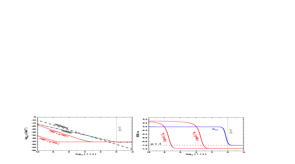
Figure 3: In the coupled YMC dark energy models, the evolution of the YMC energy density (left panels) and EOS (right panels) for the models with different initial conditions.

IV.2.2 $Q\propto H\rho_{m}$

Now, let us turn to the interaction cases with $Q\propto H\rho_{m}$, which is equivalent to the form $f(x,y)=\beta x$. The dynamical equations in (31) and (32) becomes

$$y^{\prime} = -\frac{4y}{2+y}-\frac{\beta x}{(2+y)e^{y}},$$ (47)

$$x^{\prime} = (\beta-3)x.$$ (48)

If we consider the simplest, where $\beta$ is a constant, the equation (48) follows that $x\propto a^{\beta-3}$. From the definition of $x$, we derive that $\rho_{m}\propto a^{\beta-3}$. When $\beta=0$, the model returns to the free YMC cases, and $\rho_{m}\propto a^{-3}$ as usual. However, when $\beta\neq 0$, the evolution of the dust component is changed, which is conflicted with the evolution of dust in the standard hot big-bang model. So it is dangerous to consider this kind of interaction term in the early stage of the universe.

However, it is allowed to consider the form of $Q\propto H\rho_{m}$ as a kind of phenomenological model in the late stage of the universe. The critical point ($y_{c},x_{c}$) of (47) and (48) is obtained by imposing the condition $y^{\prime}_{c}=x^{\prime}_{c}=0$, we find these is no solution at all. So we conclude that, it is impossible to obtain an attractor solution for this kind of system.

IV.2.3 $Q\propto H(\rho_{y}+\rho_{m})$

In the end, let us discuss the another kind of phenomenological model, where $Q\propto H(\rho_{y}+\rho_{m})$ is satisfied. This is equivalent to set the form $f(x,y)=\gamma[(y+1)e^{y}+x]$. We consider the simplest case, where $\gamma$ is a non-zero dimensionless constant. In the dark energy dominant stage, this system returns to the first case with $Q\propto H\rho_{y}$, and in the dust dominant stage, it returns to the second case with $Q\propto H\rho_{m}$. Similar to the second case, if we directly apply this system to the early universe, the evolution of dust would be changed, which is conflicted with the prediction of the standard hot big-bang models.

In this paper, we also consider this interaction form as a kind of phenomenological model in the late stage of the universe. The dynamical equations in (31) and (32) becomes

$$y^{\prime} = -\frac{4y}{2+y}-\frac{\gamma[(y+1)e^{y}+x]}{(2+y)e^{y}},$$ (49)

$$x^{\prime} = -3x+\gamma[(y+1)e^{y}+x].$$ (50)

From the equations (34) and (35), we obtain the critical point

$$y_{c}=\frac{3\gamma}{\gamma-12},~{}~{}x_{c}=-\frac{4y_{c}}{3}e^{y_{c}}.$$ (51)

The fractional energy density and the EOS of the YMC at this critical point are

$$\Omega_{y}=-\frac{1}{w_{y}}=\frac{3-\gamma}{3}.$$ (52)

The constraint of $0\leq\Omega_{y}\leq 1$ requires that $0<\gamma\leq 3$. In order to keep this critical point being stable, i.e. ($y_{c},x_{c}$) is the attractor solution, another constraint of $\gamma$ can be derived: $\gamma>-120/31$, which is auto-satisfied when $0<\gamma\leq 3$ is required. So the attractor solution requires that the constraint on the coefficient being

$$0<\gamma\leq 3,$$ (53)

which follows that, the EOS of YMC in this attractor solution must be negative. If we still require that, the fraction density of YMC is larger than the value at the present stage, i.e. $\Omega_{y}>0.73$, the constraint on $\alpha$ becomes much tighter $0<\gamma<0.81$.

V Statefinder and $Om$ diagnosis in the YMC models

Figure 4: Left panel: The $r-s$ diagram of the YMC models; Middle panel: The $r-q$ diagram of the YMC models; The right panel: $Om(z)$ diagnostic in the YMC models.

In this section, we shall present the way to discriminate between the YMC models and the other dark energy models. In the previous works statefinder om , the authors suggested to use the so-called “statefinder” $\{r,s\}$ pair and $Om$ diagnostics. Here, we shall also apply the statefinder diagnosis into the YMC models. The similar discussion can be found in the previous works zijmpd2008 wzxjcap2008 tzxijmpd2009 tzprd2008 .

The statefinder diagnostic pair $\{r,s\}$ is defined as

$$r\equiv\frac{\dddot{a}}{aH^{3}},~{}~{}s\equiv\frac{r-1}{3(q-1/2)},$$ (54)

where $q=-\ddot{a}/(aH^{2})$ is the deceleration parameters. $r$ forms the next step in the hierarchy of geometrical cosmological parameters beyond $H$ and $q$, and $s$ is a linear combination of $r$ and $q$. Apparently, the statefinder parameters depends only on scale factor $a$ and its derivatives, and thus it is a geometrical diagnostic. These parameters can also been expressed in terms of $\rho_{tot}$ and $p_{tot}$ as follows

$$q=\frac{1}{2}\left(1+\frac{3p_{tot}}{\rho_{tot}}\right),~{}~{}r=1+\frac{9(\rho_{tot}+p_{tot})\dot{p}_{tot}}{2\dot{\rho}_{tot}p_{tot}},~{}~{}s=\frac{\rho_{tot}+p_{tot}}{p_{tot}}\frac{\dot{p}_{tot}}{\dot{\rho}_{tot}}.$$ (55)

By using Eqs. (28) and (29), we plot the trajectories of $(r,s)$ and of $(r,q)$ in Fig. 4 from the redshift $z=10$, where we have considered two cases with $Q=0$ and $Q=0.5H\rho_{y}$. The arrows along the curves indicate the direction of evolution. In both cases, we have chosen the initial condition at the redshift $z=3454$, where the densities of matter and radiation equate to each other. We choose the initial condition to make the $\Omega_{y}=0.01$ at this high redshift.

From this figure, we find that, the model with different interaction terms have the difference in both $(r,s)$ and $(r,q)$ trajectories. However, in the low redshift ($z<10$), especially when $z\sim 0$, the trajectories in both models become quite close to those of the $\Lambda$CDM model. However, we should also mention that, the trajectories of the statefinder shows in this figure are quite different from the other dark energy models, such as the decaying vacuum model, the Quintessence models, the K-essence models (see for instant tzprd2008 ). In order to break the degeneracy between the YMC models and the $\Lambda$CDM models, let us consider the $Om$ diagnostic, which is defined as

$$Om(x)=\frac{h^{2}(x)-1}{x^{3}-1},$$ (56)

where $x\equiv(1+z)$, and $h(x)\equiv H(x)/H_{0}$. Thus $Om$ involves only the first derivative of the scale factor through the Hubble parameter and is easier to reconstruct from the observational data. For the $\Lambda$CDM model, it is simple, i.e. $Om(x)=\Omega_{m}$, independent of the redshift. For YMC model, we plot $Om$ as a function of $z$ in the Fig.4 (right panel). It is interesting to find that, for either model, $Om$ is nearly a constant at the low redshift. For the model without interaction, as expected, $Om\simeq 0.27$, very close to that of $\Lambda$CDM models. However, for the model with $Q=0.5H\rho_{y}$, $Om=0.15$, which is helpful to differentiate the coupled YMC models from the $\Lambda$CDM model.

VI Conclusion

In order to answer the observed accelerating expansion of the universe in the present stage, we introduce the quantum Yang-Mills condensate dark energy models. Different from the general scalar field models, the quantum Yang-Mills fields are the indispensable cornerstone to particles, and the Lagrangian of the Yang-Mills field is predicted by quantum corrections according to field theory.

In this paper, we review the main characters of the YMC dark energy models, where both free YMC model and possible coupled YMC models are considered. In all these models, the EOS of YMC is close to $w_{y}=1/3$ in the early stage, and tracked the evolution of radiation components. In the late stage, the value of $w_{y}$ runs to the attractor solution with $w_{y}=-1$ for the free YMC model, or with $w_{y}<-1$ for the coupled YMC models. This naturally explains the observations. The present state of the universe is independent of the initial state of Yang-Mills field, and the coincidence problem is naturally avoided. In the coupled YMC models, not only the state of $w_{y}<-1$ can be naturally realized, mildly suggested by observations, but also the ‘big-rip’ problem is auto-avoided. The most importance we should mention is that, as a dynamic dark energy model motivated by quantum effective YM field Lagrangian, all the YM models based upon 1-loop, 2-loop, and 3-loop quantum corrections, respectively, have similar dynamic behaviors. That is, the main properties of YM model for dark energy remain stable when the number of loops for quantum corrections increases up to 3-loop.

However, in all the models, the fine-tunning problem still exists, i.e. the value of $\kappa\sim 10^{-5}$eV², which is too low comparing with the typical scales in particle physics. We should notice that, this problem exists in nearly all the dark energy models, which may suggest a new physics at this low energy scale.

References

- (1) M. Kowalski, et al. (2008). Improved Cosmological Constraints from New, Old and Combined Supernova Datasets. Astrophysical Journal, 686, 749. [arXiv:0804.4142 ]
- (2) E. Komatsu, et al. (2009). Five-Year Wilkinson Microwave Anisotropy Probe (WMAP) Observations: Cosmological Interpretation. Astrophysical Journal Supplement Series, 180, 330. [arXiv:0803.0547]
- (3) M. Tegmark, et al. (2006). Cosmological Constraints from the SDSS Luminous Red Galaxies. Physical Review D, 74, 123507. [astro-ph/0608632]
- (4) T. Padmanabhan, (2006). Dark Energy: Mystery of the Millennium. Albert Einstein Century International Conference, 861, 179. [astro-ph/0603114]
- (5) D. Huterer, & A. Cooray, (2005). Uncorrelated Estimates of Dark Energy Evolution. Physical Review D, 71, 023506. [astro-ph/0404062]
- (6) A. Albrecht, et al. (2006). Report of the Dark Energy Task Force. arXiv:astro-ph/0609591.
- (7) E. J. Copeland, M. Sami, & S. Tsujikawa, (2006). Dynamics of Dark Energy. International Journal of Modern Physics D, 15, 1753. [hep-th/0603057]
- (8) I. Zlatev, L. Wang, & P. J. Steinhardt, (1999). Quintessence, Cosmic Coincidence, and the Cosmological Constant. Physical Review Letters, 82, 896. [astro-ph/9807002]
- (9) R. R. Caldwell, (2002).A Phantom Menace? Cosmological Consequences of a Dark Energy Component with Super-negative Equation of State. Physics Letters B, 545, 23. [astro-ph/9908168]
- (10) B. Feng, X. L. Wang, & X. M. Zhang, (2005). Dark Energy Constraints from the Cosmic Age and Supernova. Physics Letters B, 607, 35; [astro-ph/0404224] W. Zhao, & Y. Zhang, (2006). Quintom models with an equation of state crossing -1. Physical Review D, 73, 123509. [astro-ph/0604460]
- (11) S. M. Carroll, M. Hoffman, & M. Trodden, (2003). Can the Dark Energy Equation-of-state Parameter w Be Less Than -1? Physical Review D, 68, 023509. [astro-ph/0301273]
- (12) Caldwell, R. R.; Kamionkowski, M. & Weinberg, N. N. (2003). Phantom Energy and Cosmic Doomsday. Physical Review Letters, 91, 071301. [astro-ph/0302506]
- (13) S. M. Carroll, V. Duvvuri, M. Trodden & M. S. Turner, (2004). Is Cosmic Speed-Up Due to New Gravitational Physics? Physical Review D, 70, 043528; [astro-ph/0306438] S. M. Carroll, et al. (2005). The Cosmology of Generalized Modified Gravity Models. Physical Review D, 71, 063513. [astro-ph/0410031]
- (14) T. Chiba, T. L. Smith, & A. L. Erickcek, (2007). Solar System Constraints to General f(R) Gravity. Physical Review D, 75, 124014. [astro-ph/0611867]
- (15) C. Armendariz-Picon, (2004). Could Dark Energy Be Vector-like? Journal of Cosmology and Astroparticle Physics, 0407, 007; [astro-ph/0405267] H. Wei & R. G. Cai, (2006). Interacting Vector-like Dark Energy, the First and Second Cosmological. Physical Review D, 73, 083002; [astro-ph/0603052] H. Wei & R. G. Cai, (2007). Cheng-Weyl Vector Field and its Cosmological Application. Journal of Cosmology and Astroparticle Physics, 0709, 015; [astro-ph/0607064] M. Chaves & D. Singleton, (2008). A Unified Model of Phantom Energy and Dark Matter, arXiv:0801.4728; K. Bamba, S. Nojiri, & S. D. Odintsov, (2008). Inflationary Cosmology and the Late-time Accelerated Expansion of the Universe in Nonminimal Yang-Mills-F(R) Gravity and Nonminimal Vector-F(R) Gravity. Physical Review D, 77, 123532; [arXiv:0803.3384] T. S. Koivisto, & D. F. Mota, (2008). Vector Field Models of Inflation and Dark Energy. arXiv:0805.4229; D. V. Gal’tsov, (2009). Non-Abelian Condensates As Alternative for Dark Energy. arXiv:0901.0115; V. A. De Lorenci, (2009). Nonsingular and Accelerated Expanding Universe from Effective Yang-Mills Theory. arXiv:0902.2672; Y. Zhang, (2009). The Slow-Roll and Rapid-Roll Conditions in The Space-likeVector Field Scenario. arXiv:0903.3269; T. S. Koivisto & N. J. Nunes, (2009). Three-form Cosmology. arXiv:0907.3883; N. J. Nunes & T. S. Koivisto, (2009). In ation and Dark Energy from Three-forms. arXiv:0908.0920.
- (16) M. C. Bento, O. Bertolami, P. V. Moniz, J. M. Mourao & P.M. Sa, (1993). On the Cosmology of Massive Vector Fields with SO(3) Global Symmetry. Classical and Quantum Gravity, 10, 285; [gr-qc/9302034] E. Elizalde, J. E. Lidsey, S. Nojiri, & S. D. Odintsov, (2003). Born-Infeld Quantum Condensate as Dark Energy in the Universe. Physics Letters B, 571, 1; [hep-th/0307177] V. V. Kiselev, (2004). Vector Field as a Quintessence Partner. Classical and Quantum Gravity, 21, 3323; [gr-qc/0402095] M. Novello, S. E. P. Bergliaffa & J. Salim, (2004). Non-linear Electrodynamics and the Acceleration of the Universe. Physical Review D, 69, 127301; [astro-ph/0312093] C. G. Boehmer & T. Harko, (2007). Dark Energy as a Massive Vector Field. The European Physical Journal C, 50, 423; [gr-qc/0701029] J. B. Jimenez & A. L. Maroto, (2008). A Cosmic Vector for Dark Energy. Physical Review D, 78, 063005; [arXiv:0801.1486] J. B. Jimenez, R. Lazkoz & A. L. Maroto, (2009). Cosmic Vector for Dark Energy: Constraints from SN, CMB and BAO. arXiv:0904.0433; J. B. Jimenez, & A. L. Maroto, (2009). Cosmological Evolution in Vector-tensor Theories of Gravity. arXiv:0905.1245; K. Dimopoulos, M. Karciauskas & J. M. Wagstaff, (2009). Vector Curvaton with Varying Kinetic Function. arXiv:0907.1838; J. B. Jimenez, T. S. Koivisto, A. L. Maroto & D. F. Mota, Perturbations in electromagnetic dark energy. arXiv:0907.3648.
- (17) Y. Zhang, (1994). Inflation with Quantum Yang-Mills Condensate. Physics Letters B, 340, 18; Y. Zhang, (1996). An Exact Solution of a Quark Field Coupled with a Yang - Mills Field in de Sitter Space. Classical and Quantum Gravity, 13, 2145; Y. Zhang, (2003). Dark Energy Coupled with Relativistic Dark Matter in Accelerating Universe. Chinese Physics Letters, 20, 1899.
- (18) S .L. Adler, (1981). Effective-action Approach to Mean-field non-Abelian statics, and a Model for Bag Formation. Physical Review D, 23, 2905; S. L. Adler, (1983). Short-distance Perturbation Theory for the Leading Logarithm Models. Nuclear Physics B, 217, 381.
- (19) H. Pagels,& E .Tomboulis, (1978). Vacuum of the Quantum Yang-Mills Theory and Magnetostatics. Nuclear Physics B, 143, 485.
- (20) W. Zhao, & Y. Zhang, (2006). The State Equation of the Yang-Mills Field Dark Energy Models. Classical and Quantum Gravity, 23, 3405. [astro-ph/0510356]
- (21) W. Zhao, & Y. Zhang, (2006). Coincidence Problem in YM Field Dark Energy Model. Physics Letters B, 640, 69. [astro-ph/0604457]
- (22) S. G. Matinyan, & G. K. Savvidy, (1978). Vacuum Polarization Induced by the Intense Gauge Field. Nuclear Physics B, 134, 539.
- (23) D. J. Gross, & Wilczez, F. (1973). Ultraviolet Behavior of Non-Abelian Gauge Theories. Physical Review Letters, 30, 1343; D. J. Gross,(1973). Asymptotically Free Gauge Theories. I. Physical Review D, 8, 3633.
- (24) T. Y. Xia, & Y. Zhang, (2007). 2-loop Quantum Yang-Mills Condensate As Dark Energy. Physics Letters B, 656, 19. [arXiv:0710.0077]
- (25) S. Wang, Y. Zhang, & T. Y. Xia, (2008). 3-loop Yang-Mills Condensate Dark Energy Model and its Cosmological Constraints. Journal of Cosmology and Astroparticle Physics, 10, 037. [arXiv:0803.2760]
- (26) W. Zhao, & D. H. Xu, (2007). Evolution of Magnetic Component in Yang-Mills Condensate Dark Energy Models. International Journal of Modern Physics D, 16, 1735. [gr-qc/0701136]
- (27) W. Zhao, (2008). Statefinder Diagnostic for Yang-Mills Dark Energy Model. International Journal of Modern Physics D, 17, 1245. [arXiv:0711.2319]
- (28) M. L. Tong, Y. Zhang, & T. Y. Xia, T. (2009). Statefinder Parameters for Quantum Effective Yang-Mills Condensate Dark Energy Model. International Journal of Modern Physics D, 18, 797. [arXiv:0809.2123]
- (29) W. Zhao, (2009). Perturbations of the Yang-Mills Field in the Universe. Research in Astronomy and Astrophysics, 9, 874. [astro-ph/0508010]
- (30) A. Vikman, (2005). Can Dark Energy Evolve to the Phantom? Physical Review D, 71, 023515. [astro-ph/0407107]
- (31) R. H. Cyburt, B. D. Fields, K. A. Olive, & E. Skillman, (2005). New BBN Limits on Physics Beyond the Standard Model from He4. Astroparticle Physics, 23, 313. [astro-ph/0408033]
- (32) Y. Zhang, T. Y. Xia, & W. Zhao, (2007). Yang-Mills Condensate Dark Energy Coupled with Matter and Radiation. Classical and Quantum Gravity, 24, 3309. [gr-qc/0609115]
- (33) B. Wang, et al. (2007). Interacting Dark Energy and Dark Matter: Observational Constraints From Cosmological Parameters. Nuclear Physics B, 778, 69; [astro-ph/0607126] J. H. He,; B. Wang, & P. Zhang, (2009). The Imprint of the Interaction Between Dark Sectors in Large Scale Cosmic Microwave Background Anisotropies. arXiv:0906.0677.
- (34) W. Zhao, (2009). Attractor Solution in Coupled Yang-Mills Field Dark Energy Models. International Journal of Modern Physics D, 18, 1331. [arXiv:0810.5506]
- (35) V. Sahni, T. D. Saini, A. A. Starobinsky, & U. Alam, (2003). Statefinder - A New Geometrical Diagnostic of Dark Energy. JETP Letters, 77, 201. [astro-ph/0201498]
- (36) V. Sahni, A. Shafieloo, & A. A. Starobinsky, (2008). Two New Diagnostics of Dark Energy. Physical Review D, 78, 103502. [arXiv:0807.3548]
- (37) M. L. Tong, & Y. Zhang, (2009). Cosmic Age, Statefinder and Diagnostics in the Decaying Vacuum Cosmology. Physical Review D, 80, 023503. [arXiv:0906.3646]