Why are nonlinear fits so challenging?

Abstract

Fitting model parameters to experimental data is a common yet often challenging task, especially if the model contains many parameters. Typically, algorithms get lost in regions of parameter space in which the model is unresponsive to changes in parameters, and one is left to make adjustments by hand. We explain this difficulty by interpreting the fitting process as a generalized interpolation procedure. By considering the manifold of all model predictions in data space, we find that cross sections have a hierarchy of widths and are typically very narrow. Algorithms become stuck as they move near the boundaries. We observe that the model manifold, in addition to being tightly bounded, has low extrinsic curvature, leading to the use of geodesics in the fitting process. We improve the convergence of the Levenberg-Marquardt algorithm by adding geodesic acceleration to the usual step.

The estimation of model parameters from experimental data is astonishingly challenging. A nonlinear model with tens of parameters, fit (say) by least-squares to experimental data, can take weeks of hand-fiddling before a qualitatively reasonable agreement can be found; even then, the parameters cannot usually reliably be extracted from the data. Both general minimization algorithms and algorithms like Levenberg-Marquardt that are designed for least-squares fits routinely get lost in parameter space. This becomes a serious obstacle to progress when one is unsure of the validity of the model, e.g. in systems biology where one wants to automatically generate and explore a variety of alternative models.

Here we use differential geometry to explain why fits are so hard. We first explore the structure of the model manifold $\mathcal{M}$, the manifold of predictions embedded in the space of data, $D$, and find that it is typically bounded, with cross sections having a hierarchy of widths, so that the overall structure is similar to that of a long, thin ribbon. We explain this hierarchy by viewing the fitting process as a generalized interpolation procedure with few effective model degrees of freedom. We interpret the difficulty in fitting to be due to algorithms getting stuck near the boundary of $\mathcal{M}$, where the model is unresponsive to variations in the parameters. We then discuss how geometry motivates algorithms to alleviate this difficulty.

A typical nonlinear least squares problem fits a model $Y_{m}(\theta)$ with $N$ parameters $\theta$ to $M$ experimental data points $y_{m}$. We define the model manifold, $\mathcal{M}$, as the parametrized $N$-dimensional surface $\vec{Y}(\theta)$ embedded in Euclidean data space, $D=\mathbb{R}^{M}$. The best fit to the experiment is given by the point on $\mathcal{M}$ with Euclidean distance closest to the data, minimizing the cost $C=\frac{1}{2}(\vec{Y}(\theta)-\vec{y})^{2}$. The Euclidean metric of data space (with distance between models given by the change in residuals, $\vec{r}=\vec{Y}(\theta)-\vec{y}$) induces a metric on the manifold, $g_{\mu\nu}=\partial_{\mu}\vec{Y}\cdot\partial_{\nu}\vec{Y}=(J^{T}J)_{\mu\nu}$, where $J_{m\mu}=\frac{\partial}{\partial\theta_{\mu}}Y_{m}$; $g_{\mu\nu}$ is known as the Fisher Information matrix. As an example, the model $Y(t,\theta)=f_{\theta}(t)=e^{-\theta_{1}t}+e^{-\theta_{2}t}$ sampled at three time points is given in Fig. 1. The model manifold has been extensively studied by the information geometry statistics community Amari2007 , but they focus on the intrinsic curvature; as the cost is the distance in data space, the embedding and its extrinsic curvature are crucial to finding best fits Bates1980 ; Bates1988 .

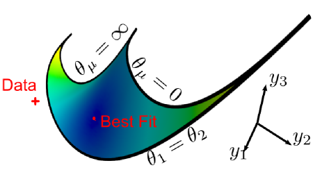
Figure 1: The model manifold for the two-exponential problem, with $y_{i}$ evaluated at $t=1/3$, $1$, and $3$. Boundaries exist when $\theta_{\mu}=0,\infty$ and when $\theta_{1}=\theta_{2}$. (The ribbon-like structure of Fig. 2 emerges only in higher dimensions.)

As seen in figs. 2 and 3, this model manifold can take the form of a hyper-ribbon, with thinnest direction four orders of magnitude smaller than the long axes. To understand this observed hierarchy, consider the special case of analytic models, $f(t,\theta)$, of a single independent variable (time) where the data points are $Y_{m}=f(t_{m})$. Let $R$ be the typical time scale over which the model behavior changes, so that the $n^{th}$ term of the Taylor series $f^{(n)}(t)/n!\lesssim R^{-n}$ (roughly the radius of convergence). If the function is sampled at $n$ time point $(t_{1},t_{2},...,t_{n})$ within this time scale, the Taylor series may be approximated by the unique polynomial of degree $n-1$, $P_{n-1}(t)$ passing through these points. At a new point, $t_{0}$, the discrepancy between the interpolation and the function is given by

$$f(t_{0})-P_{n-1}(t_{0})=\omega_{n}(t_{0})f^{(n)}(\xi)/n!,$$ (1)

where $\xi$ lies somewhere in the interval containing $t_{0},\ t_{1},\ ...,\ t_{n}$ Stoer2002 . The polynomial $\omega_{n}(t)$ has roots at each of the interpolating points $\omega_{n}(t)=(t-t_{1})(t-t_{2})...(t-t_{n}).$ The possible error of the interpolation function bounds the allowed range of behavior, $\Delta f_{n}$, of the model at $t_{0}$ after constraining the nearby $n$ data points (i.e. cross sections). Consider the ratio of successive cross sections, $\frac{\Delta f_{n+1}}{\Delta f_{n}}=(t-t_{n+1})(n+1)\frac{f^{n+1}(\xi)}{f^{n}(\xi^{\prime})}.$ If $n$ is sufficiently large, then $(n+1)\frac{f^{n+1}(\xi)}{f^{n}(\xi^{\prime})}\approx\frac{1}{R}$; therefore, we find that $\frac{\Delta f_{n+1}}{\Delta f_{n}}\approx\frac{t-t_{n+1}}{R}<1$ by the ratio test. Each cross section is thinner than the last by a roughly constant factor, yielding the observed hierarchy.

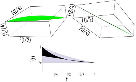
Figure 2: Top: Two views of the cross section of the model manifold for an infinite sum of exponentials $F_{{\mathbf{A}},{\mathbf{\theta}}}(t)=\sum_{n}A_{n}\exp(-\theta_{n}t)$ with $A_{n}\geq 0$, given by fixing $F(0)=1$ and $F(1)=1/e$. Bottom: The range of allowed fits (grey) is strongly reduced by fixing the output at $t=1/2$ to the midpoint of its range (black).

We argue that this hyper-ribbon structure will be shared with a wide variety of nonlinear, multiparameter models. Note that the eigenvalues of the metric tensor $g_{\mu\nu}$ in Fig. 3 also form a hierarchy, spanning eight orders of magnitude – this ‘sloppiness’ has been documented in a number of other models, including seventeen in systems biology Gutenkunst2007a , insect flight and variational quantum wave functions Waterfall2006 , interatomic potentials Frederiksen2004 , and a model of the next-generation international linear collider Gutenkunst2008 . (Multiparameter models whose parameters are individually measured by the data, and on the other extreme models with sensitive, chaotic dependence on parameters, will likely not fall into this family.) Most parameters in these models have bounded effects – they can be set to limiting values (zero, infinity, etc.) and still have finite model predictions – rates and Michaelis-Menten coefficients in systems biology, Jastrow and determinential factors in variational wave functions, etc. Note that the widths of the model manifold track nicely with these eigenvalues in Fig. 3 (taking the square root to match units): moving parameter combinations along eigendirections of the metric by an order of magnitude (fixed shift in log parameters) exhausts the range of behavior (width). This tracking suggests that the ubiquity of sloppy eigenvalue spectra at best fits implies a ubiquitous hyper-ribbon structure for the model manifold.

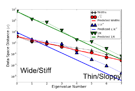
Figure 3: Geodesic cross-sectional widths of an eight dimensional model manifold along the eigendirections of the metric from some central point, together with the square root of the eigenvalues (singular values of the Jacobian), the inverse extrinsic (geodesic) curvature $K$ Spivak1979 , and the inverse geodesic parameter-effects curvature $K^{P}$ Bates1980 ; Bates1988 ; Transtrum2010 . Notice the hierarchy of these data-space distances – the widths and singular values each spanning around four orders of magnitude and the curvatures covering eight. Note also that the extrinsic curvatures are three orders of magnitude smaller than the parameter-effects curvature.

Our observation that many models are sloppy, presumably sharing this hyper-ribbon model manifold structure, is now explained: multiparameter models are a kind of high-dimensional analytic interpolation scheme, and near degenerate Hessians result whenever multiple data points reside within some generalized radius of convergence. When this is the case, the data points are highly correlated and the model has few effective degrees of freedom. Whenever there are many model parameters for each effective degree of freedom there will be a hierarchy of widths and the model will be sloppy.

Our geometric interpretation explains a number of observations about nonlinear models. First, although parameters cannot be reliably extracted by fitting degenerate models, it is still possible to constrain the outcome of new experiments Brown2003a ; Gutenkunst2007a . Because the fitting process is an interpolation scheme, only a few stiff parameter combinations need to be tuned to fit most of the data, since only a few data points constrain the predictions at other times. The remaining unconstrained parameter combinations control the interpolated values, which are already restricted by the analyticity of the model.

Figure 3 also shows that the parameter effects curvature Bates1980 ; Bates1988 ; Transtrum2010 and the geodesic extrinsic curvatures vary over twice as many decades as the widths and $\sqrt{\lambda}$; indeed, their formulas include a factor of $1/\lambda$. Why is the extrinsic curvature so much smaller? The manifold has zero extrinsic curvature if there are equal numbers of parameters as data points, $N=M$ (where the model manifold is a sub-volume in the Euclidean data space). We have seen that most of the data points are interpolations that supply little new information; the extrinsic curvature will be small when the effective dimensionality of the embedding space is not larger than than the number of parameters.

We use geodesics to construct new polar coordinates $\gamma^{\mu}=\gamma^{\mu}(\theta)$ on $\mathcal{M}$ that generalize Riemann normal coordinates Misner1973 . Since geodesics are nearly straight lines in data space on $\mathcal{M}$, we find that cost contours in these coordinates are nearly quadratic and isotropic around the best fit, as explicitly computed in Fig. 4. Nonlinear models locally look like linear models with badly chosen parameters, well beyond the harmonic approximation.

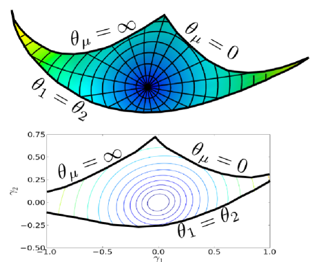
Figure 4: Geodesics can be used to construct polar coordinates on $\mathcal{M}$ (above). In these new geodesic coordinates, the cost contours are nearly perfect, isotropic circles (below).

Can these nearly straight geodesics inspire algorithms that lead efficiently to the best fit? Integrating the geodesic equation with a single Euler step reproduces the Gauss-Newton step ($\delta\theta^{\mu}=-g^{\mu\nu}\nabla_{\nu}C$ in our notation), ineffective due to the large eigenvalues in the inverse metric $g^{\mu\nu}$; even geodesic motion hits the boundaries of $\mathcal{M}$. The ribbon is nearly flat, but very thin; the geodesics hit the edges long before finding a good fit.

To improve convergence, we can modify the model manifold to remove the boundaries. One method of doing this is to introduce the model graph $\mathcal{G}$, which is the $N$-dimensional parametric surface drawn by the model embedded in data space crossed with parameter space. Since most boundaries occur at infinite parameter values, the model graph $\mathcal{G}$ ‘stretches’ these boundaries to infinity in the parameter space portion of the embedding. The metric for the model graph is an interpolation of the data space and parameter space metrics, $g_{\mu\nu}=g_{\mu\nu}^{0}+\lambda^{*}I_{\mu\nu}$, where $\lambda^{*}$ determines the weight of the two spaces. Notice that the eigendirections of the metric are the same on both $\mathcal{M}$ and $\mathcal{G}$; however, the eigenvalues on the graph are given by $\lambda_{\mathcal{G}}=\lambda_{\mathcal{M}}+\lambda^{*}$. Therefore, the degenerate eigendirections with $\lambda_{\mathcal{M}}\ll\lambda^{*}$ have eigenvalues $\lambda_{\mathcal{G}}\approx\lambda^{*}$ on the model graph; $\lambda^{*}$ cuts off the small eigenvalues of the Hessian. The analogy of the Gauss-Newton step on the model graph is the well-known Levenberg-Marquardt step, $\delta\theta=-\left(J^{T}J+\lambda^{*}I\right)^{-1}\nabla C$ in our notation Marquardt1963 ; More1977 ; Press2007 . By dynamically adjusting $\lambda^{*}$, the algorithm can shorten its step, removing the danger of the degenerate Hessian, while rotating from the Gauss-Newton direction into the steepest descents direction. Geometrically we understand the superiority of Levenberg-Marquardt to be due to the lack of boundaries of the model graph.

Algorithm	Success Rate	Mean njev	Mean nfev
Traditional LM + accel	65%	258	1494
Traditional LM	33%	2002	4003
Trust Region LM	12%	1517	1649
BFGS	8%	5363	5365

Table 1: The results of several algorithms applied to a test problem of fitting a sum of four exponential terms (varying both rates and amplitudes) in log-parameters (to enforce positivity). Initial conditions are chosen near a manifold boundary with a best fit of zero cost near the center of the manifold. Among successful attempts, we further compare the average number of Jacobian and function evaluations needed to arrive at the fit. Success rate indicates an algorithm’s ability to avoid the manifold boundaries (find the canyon from the plateau), while the number of Jacobian and function evaluations indicate how efficiently it can follow the canyon to the best fit. BFGS is a quasi newton scalar minimizer of Broyden, Fletcher, Goldfarb, and Shanno (BFGS) Nocedal1999 ; Jones2001 . The traditional Marquardt1963 ; Press2007 and trust region More1977 implementations of Levenberg-Marquardt consistently outperform this and other general optimization routines on least squares problems, such as Powell, simplex, and conjugate gradient. Including the geodesic acceleration on a standard variant of Levenberg-Marquardt dramatically increases the success rate while decreasing the computation time.

Inspired by the results in Fig. 4, we further improve the standard Levenberg-Marquardt algorithm. Interpreting the Levenberg-Marquardt step as a velocity, $v^{\mu}=-g^{\mu\nu}\nabla_{\nu}C$, where $g$ is the metric on the model graph, the geodesic acceleration (giving the parameter-effects curvature) is given by $a^{\mu}=-g^{\mu\nu}\partial_{\nu}\vec{y}\cdot\partial_{\alpha}\partial_{\beta}\vec{y}\ v^{\alpha}v^{\beta}$, giving a step $\delta\theta^{\mu}=v^{\mu}+\frac{1}{2}a^{\mu}$. The geodesic acceleration is very cheap to calculate, requiring only a directional second derivative, which can be estimated from three (cheap) function evaluations (one or two additional function evaluations) at each step with no extra (expensive) Jacobians. The geodesic acceleration serves two purposes. First, it provides an estimate for the trust region in which the linearization approximation (from which Levenberg-Marquardt is traditionally derived) is valid. At each step, we adjust $\lambda$until the acceleration is smaller than the velocity, which we find is more effective at avoiding model boundaries than either tuning until a downhill step is found Marquardt1963 ; Press2007 or considering the reduction ratio More1977 . The second benefit of the acceleration occurs when the algorithm must follow a long narrow canyon to the best fit. In these scenarios convergence may be sped up by approximating the path with a parabola instead of a line. The utility of the geodesic acceleration is seen in Table 1, where the performance of several algorithms on a test problem is summarized. More extensive comparisons and further refined algorithms are in preparation Transtrum2010b .

Just as the special sum of squares form of the cost function gives an approximate Hessian using only first derivatives of the residuals, $H\approx J^{T}J$, it has (together with the low extrinsic curvature) allowed us to approximate the cubic correction using only a directional second derivative. All other algorithms that seek to improve the Levenberg-Marquardt algorithm use second derivative information only to calculate the correction $\delta H_{\mu\nu}=\vec{r}\cdot\partial_{\mu}\partial_{\nu}\vec{r}$, to the Hessian DennisJr1977 ; Gill1978 ; DennisJr1981 ; Gonin1987 . This correction is negligible if the nonlinearities are primarily parameter-effects curvature; since the unfit data is nearly perpendicular to the surface of the model manifold while the nonlinearities are tangent to the model manifold, the dot product vanishes. Qualitatively, this means that the approximate Hessian is very accurate and that the bending of the local ellipses, (due to the third order terms in the cost that we consider) are the most important correction.

By interpreting the fitting process as a generalized interpolation scheme, we have seen that the difficulties in fitting are due to the narrow boundaries on the model manifold, $\mathcal{M}$. These boundaries form a hierarchy of widths dual to the hierarchy of Hessian eigenvalues characteristic of nonlinear model fits. Additionally, we both observe and argue that the model manifold is remarkably flat (low extrinsic curvature), which leads us to the use of geodesics in the fitting process. The modified Gauss-Newton and Levenberg-Marquardt algorithms are understood to be Euler approximations to the geodesic equation on the model manifold and model graph respectively. The geodesic acceleration improves convergence of Levenberg-Marquardt by providing a more accurate trust region while reducing computation time. Data fits are both practically important and theoretically elegant.

The authors thank Bryan Daniels, Stefanos Papanikolaou, Joshua Waterfall, Chris Myers, Ryan Gutenkunst, John Guckenheimer, and Eric Siggia for helpful discussions. This work was supported by NSF grant number DMR-0705167.

References

- (1) S. Amari, H. Nagaoka: Methods of Information Geometry: Amer Mathematical Society (2007)
- (2) D. Bates, D. Watts: J. Roy. Stat. Soc 42 (1980) 1
- (3) D. Bates, D. Watts: Nonlinear Regression Analysis and Its Applications: John Wiley (1988)
- (4) J. Stoer, R. Bulirsch, W. Gautschi, C. Witzgall: Introduction to numerical analysis: Springer Verlag (2002)
- (5) R. Gutenkunst, J. Waterfall, F. Casey, K. Brown, C. Myers, J. Sethna: PLoS Comput Biol 3 (2007) e189
- (6) J. Waterfall, F. Casey, R. Gutenkunst, K. Brown, C. Myers, P. Brouwer, V. Elser, J. Sethna: Physical Review Letters 97 (2006) 150601
- (7) S. Frederiksen, K. Jacobsen, K. Brown, J. Sethna: Physical Review Letters 93 (2004) 165501
- (8) R. Gutenkunst: Sloppiness, modeling, and evolution in biochemical networks: Ph.D. thesis, Cornell University (2008)
- (9) M. Spivak: PublishorPerish, California (1979)
- (10) M. K. Transtrum, B. B. Machta, J. P. Sethna: The geometry of nonlinear least squares with applications to sloppy models and optimization: In preparation
- (11) K. S. Brown: Signal Transduction, Sloppy Models, and Statistical Mechanics: Ph.D. thesis, Cornell University (2003)
- (12) C. Misner, K. Thorne, J. Wheeler: Gravitation: WH Freeman and Company (1973)
- (13) D. Marquardt: Journal of the Society for Industrial and Applied Mathematics 11 (1963) 431
- (14) J. More: Lecture notes in mathematics 630 (1977) 105
- (15) W. Press, S. A. Teukolsky, W. T. Vetterling, B. P. Flannery: Numerical recipes: the art of scientific computing: Cambridge University Press (2007)
- (16) J. Nocedal, S. Wright: Numerical optimization: Springer (1999)
- (17) E. Jones, T. Oliphant, P. Peterson, et al.: URL http://www. scipy. org (2001)
- (18) M. K. Transtrum, B. B. Machta, C. Umrigar, P. Nightingale, J. P. Sethna: Development and comparison of algorithms for nonlinear least squares fitting: In preparation
- (19) J. Dennis Jr, J. More: Siam Review 19 (1977) 46
- (20) P. Gill, W. Murray: SIAM Journal on Numerical Analysis (1978) 977
- (21) J. Dennis Jr, D. Gay, R. Walsh: ACM Transactions on Mathematical Software (TOMS) 7 (1981) 348
- (22) R. Gonin, S. Toit: Communications in Statistics-Theory and Methods 16 (1987) 969