Rotation shields chaotic mixing regions from no-slip walls

Abstract

We report on the decay of a passive scalar in chaotic mixing protocols where the wall of the vessel is rotated, or a net drift of fluid elements near the wall is induced at each period. As a result the fluid domain is divided into a central isolated chaotic region and a peripheral regular region. Scalar patterns obtained in experiments and simulations converge to a strange eigenmode and follow an exponential decay. This contrasts with previous experiments [Gouillart et al., Phys. Rev. Lett. 99, 114501 (2007)] with a chaotic region spanning the whole domain, where fixed walls constrained mixing to follow a slower algebraic decay. Using a linear analysis of the flow close to the wall, as well as numerical simulations of Lagrangian trajectories, we study the influence of the rotation velocity of the wall on the size of the chaotic region, the approach to its bounding separatrix, and the decay rate of the scalar.

Chaotic advection is often presented Aref (1984); Ottino (1989) as an efficient alternative to turbulence for the mixing of viscous fluids or delicate substances, as often encountered for example in the food and pharmaceutical industries. The repeated stretching and folding of fluid particles, induced for instance by mechanical stirrers, transforms an heterogeneity into a striated pattern with high gradients of the concentration field. This greatly enhances molecular diffusion, which accelerates the homogenization process. In contrast to turbulence, the velocity field that causes chaotic advection is spatially smooth and coherent in time. Fluid particles may therefore reside for long times in regions where stretching is much lower than average, before wandering to the rest of the domain. The global mixing rate is slowed down by such fluid particles whose motion is not ergodic on the typical timescales of a mixing experiment. For example, “sticky” KAM islands trap particles in their vicinity for long times Pikovsky and Popovych (2003). Recent theory groupedtheory (0000), numerical simulations groupednumerics (0000), and experiments Gouillart et al. (2007, 2008, 2009) have shown that the vicinity of a no-slip vessel wall is a region of poor stretching that can slow down the whole mixing process.

In this Letter, we present a class of time-periodic protocols exhibiting chaotic advection, but where the chaotic region is shielded from the influence of the wall. We recover the exponential decay of the scalar variance (Fig. 1(d)) and experimental concentration patterns that converge to a periodic pattern after a few periods (Fig. 2), as predicted by theories based on statistics of stretching Antonsen, Jr. et al. (1996); Balkovsky and Fouxon (1999); Thiffeault and Childress (2003) or eigenmode analysis of the advection-diffusion operator Pierrehumbert (1994); Fereday et al. (2002). On the contrary, the convergence to an eigenmode pattern was never observed on experimental timescales for a chaotic region that extends to the walls Gouillart et al. (2007, 2008). The key ingredient is that a regular region separates the chaotic region from the wall, as in Fig. 1(b) and (c). Rotating the wall at a constant angular velocity is a simple way of creating such a regular layer that insulates the chaotic region from the wall. In the present study, we investigate the case of a slowly moving wall and predict the size of the regular region, as well as the dynamics near the separatrix between chaotic and regular regions. We compare results of an analytical model with numerical simulations. Finally, we investigate the influence of the phase portrait on the dynamics of mixing and deduce an optimum for the rotation velocity.

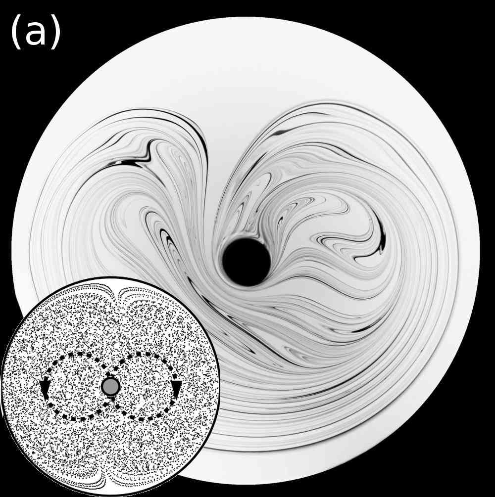
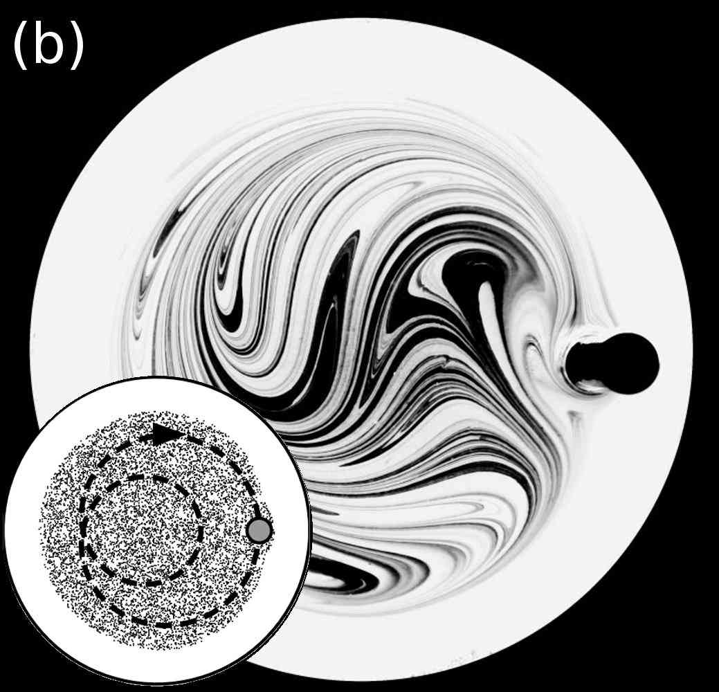
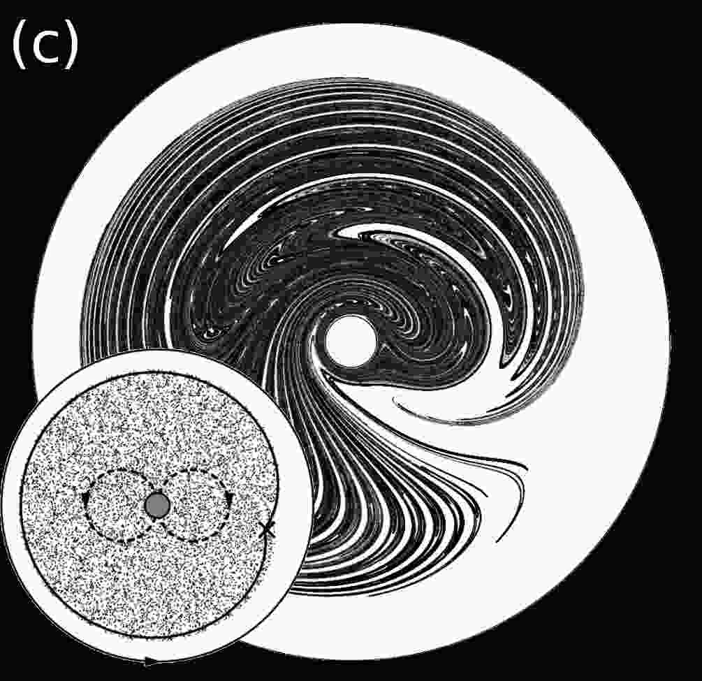
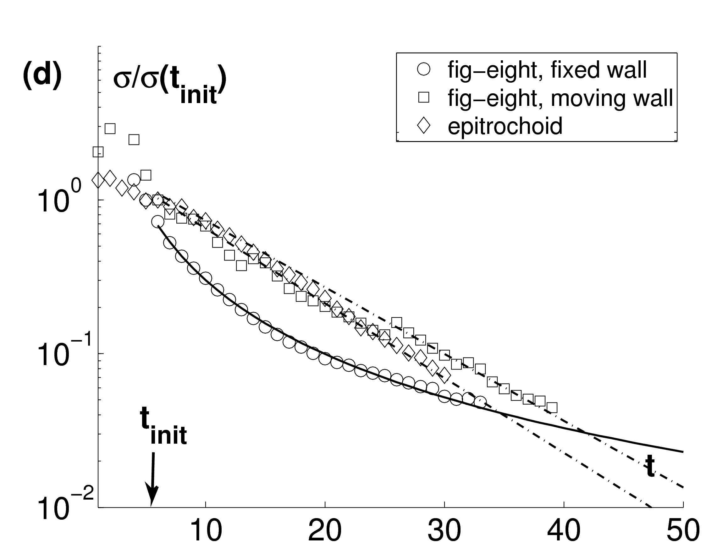
Figure 1: Chaotic mixing in a closed vessel. (a)–(b) Experiments: a rod moves periodically following (a) a figure-eight and (b) an epitrochoid path. (c) Numerical simulation of the figure-eight path with a rotating wall. Insets: Poincaré section (stroboscopic map) obtained numerically for the corresponding Stokes flow (dotted line: rod path; filled circles: fixed points of interest; solid line: associated separatrices). (d) Evolution of the standard deviation $\sigma(C)$ of the concentration, rescaled by its value at $t_{init}$, the time at which the mixing pattern emerges, for (a)–(c).

Let us first present the basic experimental and numerical observations. In all protocols, we consider two-dimensional flows with a single periodically-driven cylindrical stirrer, and an outer cylindrical wall that is either fixed or rotated at a constant angular velocity. Experimentally, the rod gently stirs viscous sugar syrup following either a figure-eight path (Fig. 1(a)) or an epitrochoid (Fig. 1(b)), that is a loop with a smaller inner loop. The fluid viscosity $\nu=5\times 10^{-4}\,\text{m}^{2}\cdot\text{s}^{-1}$ together with rod diameter $\ell=16\,\text{mm}$ and stirring velocity $U=2~{}\text{cm}\cdot\text{s}^{-1}$ yield a Reynolds number $Re=U\ell/\nu\simeq 0.6$, consistent with a Stokes-flow regime. A spot of low-diffusivity dye (India ink diluted in sugar syrup) is injected at the surface of the fluid, and we follow the evolution of the dye concentration field during the mixing process (see Fig. 1). The concentration field is measured through the transparent bottom of the vessel using a $12$-bit CCD camera at resolution $2000\times 2000$. Since our experimental set-up does not allow rotation of the vessel wall, we resort to numerical simulations of Stokes flow Finn and Cox (2001) for integrating Lagrangian trajectories of the figure-eight protocol with a rotating wall. A scalar concentration field is obtained by coarse-graining the positions of a large number ($4\times 10^{6}$) of trajectories, all initialized inside the same small spot. Figure 1(c) shows a numerically-computed concentration field for the case of a rotating wall.

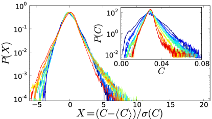
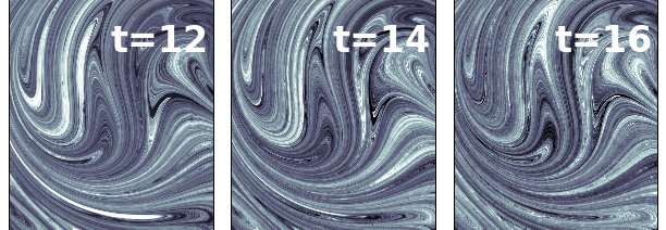
Figure 2: [Color online] Experimental evidence of an eigenmode for the epitrochoid protocol. Top: probability distribution function of the concentration. Bottom: rescaled concentration field at successive periods, showing the converged periodic pattern.

In all cases, the scalar blob, initially released in the center of the vessel, is stretched and folded into thin filaments, resulting in a complicated pattern that expands with time and gradually fills the chaotic region. The extent of the chaotic region can be seen in the numerically-computed Poincaré sections in the insets of Fig. 1(a–c). For the figure-eight protocol with fixed walls (Fig. 1(a)), the chaotic region spans the entire vessel. By contrast, the other protocols force fluid particles to follow regular closed trajectories in the vicinity of the wall, either because of the rotation of the wall itself (Fig. 1(c)), or because the epitrochoid protocol imposes a net rotational motion of the fluid elements close to the wall (Fig. 1(b)). A regular (non-chaotic) unmixed region thus separates the walls from the chaotic region in Fig. 1(b–c). This is the key factor responsible for the different evolutions of the standard deviation $\sigma(C)$ of the concentration field shown in Fig. 1(d). Statistics of the concentration field are measured in a large rectangle inside the chaotic region. In the case of the figure-eight protocol with fixed wall, the standard deviation decays algebraically, whereas it decays exponentially in the two other cases. For the epitrochoid protocol, we have experimental evidences that the concentration fields rapidly converges to an eigenmode (see Fig. 2): the probability distribution of the concentration and the concentration pattern itself rapidly become invariant. This periodic pattern is associated with the slowest-decaying Floquet eigenmode of the advection-diffusion operator Pierrehumbert (1994). By contrast, we described in Gouillart et al. (2007, 2008) how no permanent pattern can be attained in the case of a fully chaotic region, because an unmixed pool of fluid close to the wall slowly leaks into the center of the fluid domain.

In Gouillart et al. (2007, 2008), we showed how the algebraic variance decay is related to the algebraic dynamics of the flow in the vicinity of a parabolic fixed point located at the wall. In the following, we will show how the new phase portrait obtained in the presence of a net rotation within the vessel is characterized by a regular region near the wall of typical width $d$. The convergence of fluid particles to this region is exponentially fast, and we recover an exponential decrease of the variance. We focus on the figure-eight rod-stirring protocol with a moving wall, where we can tune the rotation rate of the wall independently from the rod motion. In the limit of slowly moving walls, incompressibility and the no-slip boundary condition suggest writing the flow near the wall as a simple map,

$$\bar{}\theta=\theta+\Omega+A(\theta)y,\qquad\bar{}y=y-\tfrac{1}{2}A^{\prime}(\theta)y^{2},$$ (1)

to leading order in $y$. Here $(\theta(t),y(t))$ is the position of a fluid particle at the beginning of a time interval, $(\bar{}\theta,\bar{}y)=(\theta(t+T),y(t+T))$ its new position after one stirring period $T$, and we have supposed that the fluid is incompressible. The angle $\theta$ is measured counterclockwise along the wall, $0\leq y\ll 1$ measures the distance from the wall, and $\Omega/T$ is the wall angular velocity. The circular container is assumed to have unit radius. We can regard $A(\theta)$ as the contribution of the rod motion to the velocity field near the wall. As such, $A(\theta)$ does not vary significantly when $\Omega$ changes, as long as $\Omega$ remains small (this has been confirmed numerically). $A(\theta)$ is positive where the motion of the rod and the wall reinforce each other (i.e. in the left part of the vessel in Fig. 1(c)) and negative where there is opposition between the wall and the rod (right part of the vessel). In particular, there exists a fixed point of the map (1) (a period-1 point of the flow) given by

$$A^{\prime}(\theta_{*})=0\,,\qquad y_{*}=-{\Omega}/{A(\theta_{*})}$$ (2)

where the rotating wall balances exactly the flow induced by the moving rod. This fixed point is at a distance

$$d_{*}(\Omega)={\Omega}/{\lvert A(\theta_{*})\rvert}$$ (3)

from the wall and is pictured as a small filled disk in Fig. 1(c).

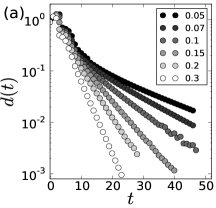
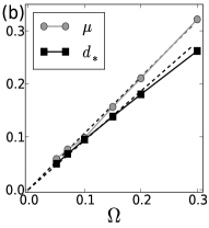
Figure 3: (a) The distance $d(t)$ from the edge of the central mixed region to the wall, for different values of $\Omega$. (b) The exponential decay rate $\mu(\Omega)$ of $d(t)$ and the distance $d_{*}(\Omega)$ separating the hyperbolic fixed point from the wall, measured from simulations (solid lines) and from Eqs. (3) and (4) (dashed lines).

The linearization matrix for the dynamics near the fixed point has eigenvalues $1\pm\mu$ with

$$\mu=\Omega\,\sqrt{-{A^{\prime\prime}(\theta_{*})}/{2A(\theta_{*})}}$$ (4)

where the argument in the square root is non-negative since $A(\theta_{*})<0$ and $A^{\prime\prime}(\theta_{*})\geq 0$. This is a hyperbolic fixed point and the approach along its stable manifold (the separatrix plotted in Fig. 1(c)) is given by

$$y(t)\sim y(0)\,\exp(-\mu\,t/T)$$ (5)

to first order in $\Omega$. The approach to the fixed point is exponential, at a rate proportional to the speed of rotation of the wall. For comparison, it was shown in Gouillart et al. (2007, 2008) that the approach to the wall scales as $1/t$ for $\Omega=0$. Figure 3(c) displays the evolution of $d(t)$, the distance separating the scalar blob from the fixed point, for simulations with different $\Omega$. One clearly observes the predicted exponential approach, with a slower rate for smaller $\Omega$ (eventually leading to an algebraic decay for $\Omega=0$). In Fig. 3(b) we show the results for $d_{*}(\Omega)$ and $\mu(\Omega)$ defined in Eqs. (3) and (4), as measured in numerical simulations. We observe a linear evolution of $d_{*}(\Omega)$ and $\mu(\Omega)$ with $\Omega$ that agrees quantitatively with Eqs. (3) and (4). Even a slow rotation of the wall ($\Omega=0.3$ corresponds to a whole rotation of the vessel in 21 periods of the rod motion) decreases the radius of the chaotic region by $25\%$. Altogether, the agreement of the above analysis with numerical simulations is excellent.

The different rates of approach are reflected in a different time-evolution for the scalar variance. To show this, we have simulated the mixing of a scalar blob for different wall velocities ($\Omega$ varying from $0.05$ to $0.4$). The evolution of the normalized standard deviation of the scalar field is measured inside a central rectangle, and plotted in Figs. 4(b–d). Fig. 4(a) offers a simplified sketch of the observed evolution. For a few initial periods ($t<t_{\mathrm{init}}$), the mixing pattern emerges and diffusion is not yet efficient. (Figs. 4(b–d) show a spurious initial ‘spike’ since the concentration is not measured in the entire domain.) For times $t>t_{\mathrm{init}}$ we observe a rapid exponential decrease of $\sigma(C)$ for all $\Omega$. After a time $t_{\mathrm{sep}}$, we observe a transition to a slower exponential regime with a rate $\alpha$ that increases with $\Omega$. The transition time $t_{\mathrm{sep}}$ decreases when $\Omega$ increases (see Figs. 4(b–d)). Increasing $\Omega$ further leads to the collapse of this second exponential regime on the continuation of the initial exponential regime (see Fig. 4(d)).

We now propose a scenario that accounts for these observations. Between $t_{\mathrm{init}}$ and $t_{\mathrm{sep}}$, diffusion starts to smear out dye filaments that are elongated by the rod motion. The decay of the variance stems from the distribution of stretching experienced by fluid particles in the bulk, as described in Antonsen, Jr. et al. (1996). Since the influence of the wall on the velocity field is weak in the region spanned by the rod’s path, the same decay regime is observed for different values of $\Omega$. At the time $t_{\mathrm{sep}}$ when some filaments arrive in the vicinity of the hyperbolic point and its separatrix (visible as a ‘knee’ in Fig. 3), fluid particles that have stayed most of the time in the core of the chaotic region have all been stretched significantly, and most of the initial variance corresponding to such fluid particles has been exhausted. However, there exists outside the central mixing pattern a pool of poorly stretched fluid delineated by the separatrix. For $t>t_{\mathrm{sep}}$, the decay of the distance $d(t)$ to this separatrix is governed by the exponential dynamics of Eq. (5), and because of area-preservation an unmixed strip of width $\Delta(t)\simeq d(t)-d(t+T)\simeq-T\,{\dot{d\mkern 8.0mu}\mkern-8.0mu}{}(t)$ must enter the central mixing region along the unstable manifold of the fixed point (see the white ‘tongue’ in Fig. 1(c)). The strip is then thinned to the Batchelor length $\ell=\sqrt{\kappa/\lambda}$, where $\kappa$ is the molecular diffusivity and $\lambda$ is an average stretching rate inside the central mixing region Batchelor (1959); Balkovsky and Fouxon (1999); Thiffeault (2008), and finally wiped out by diffusion.

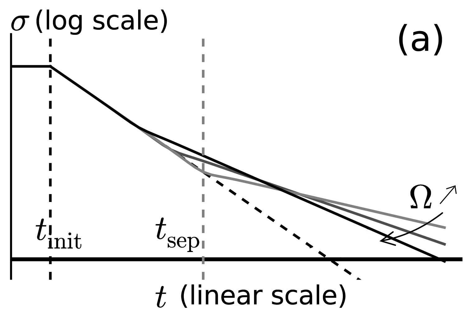
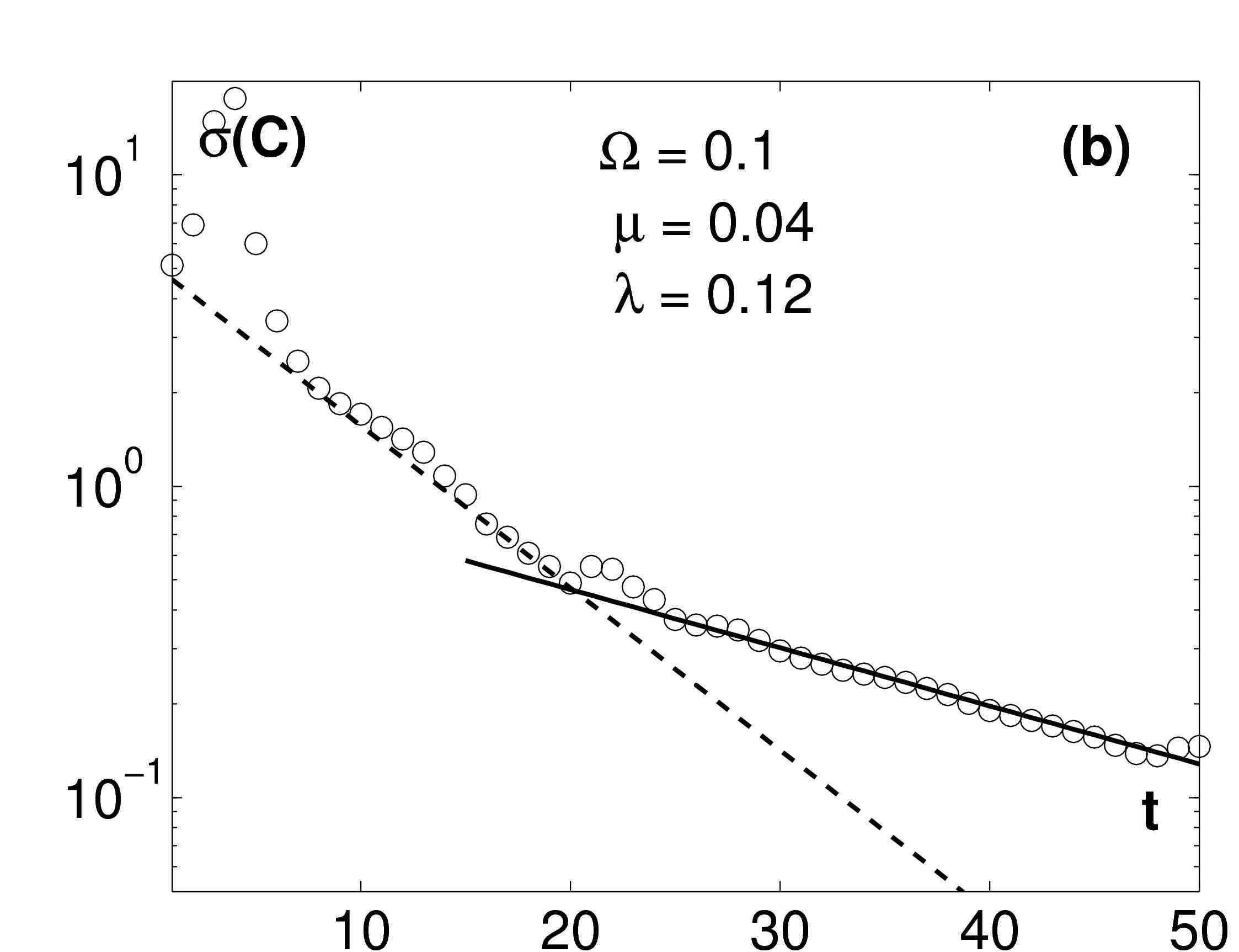
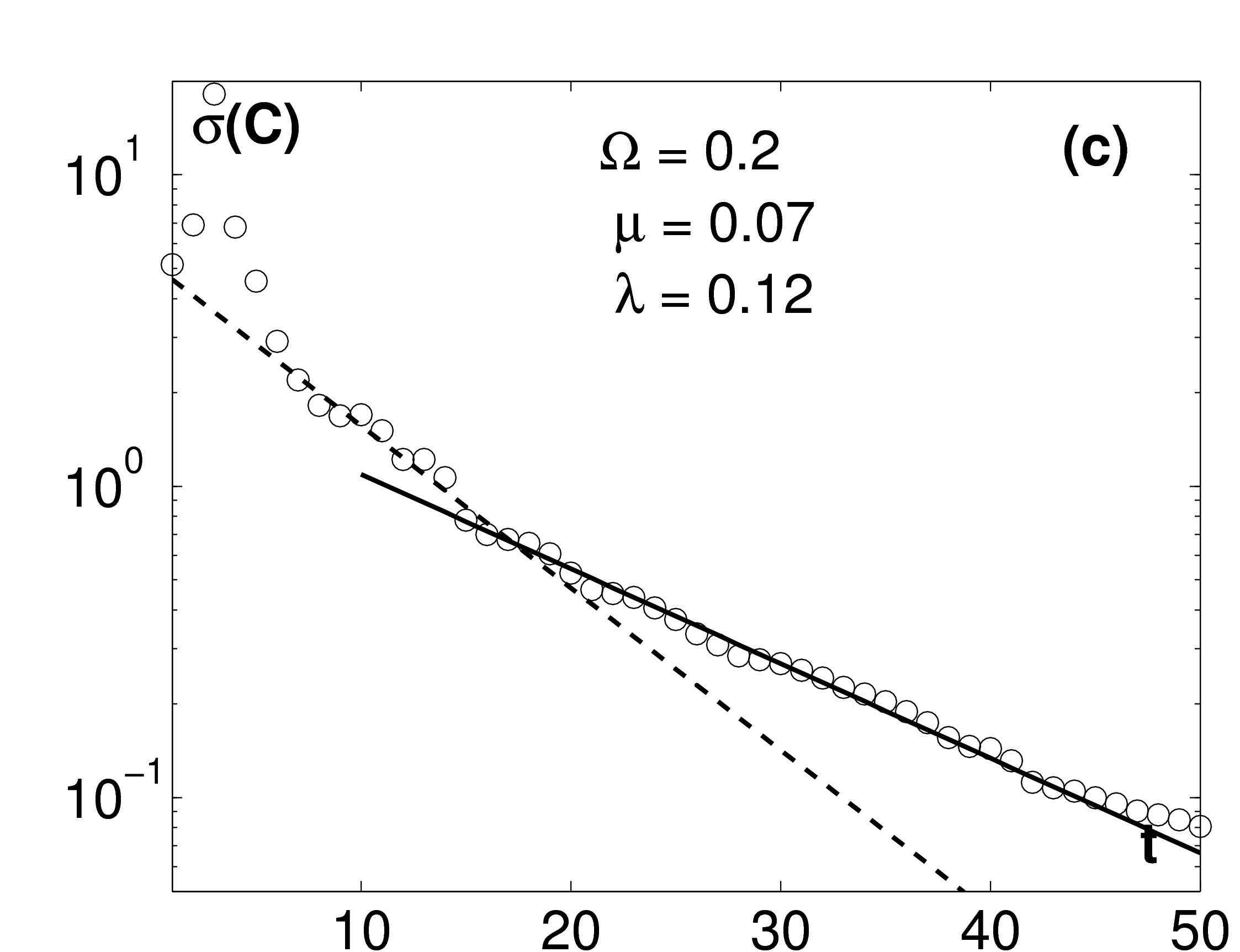
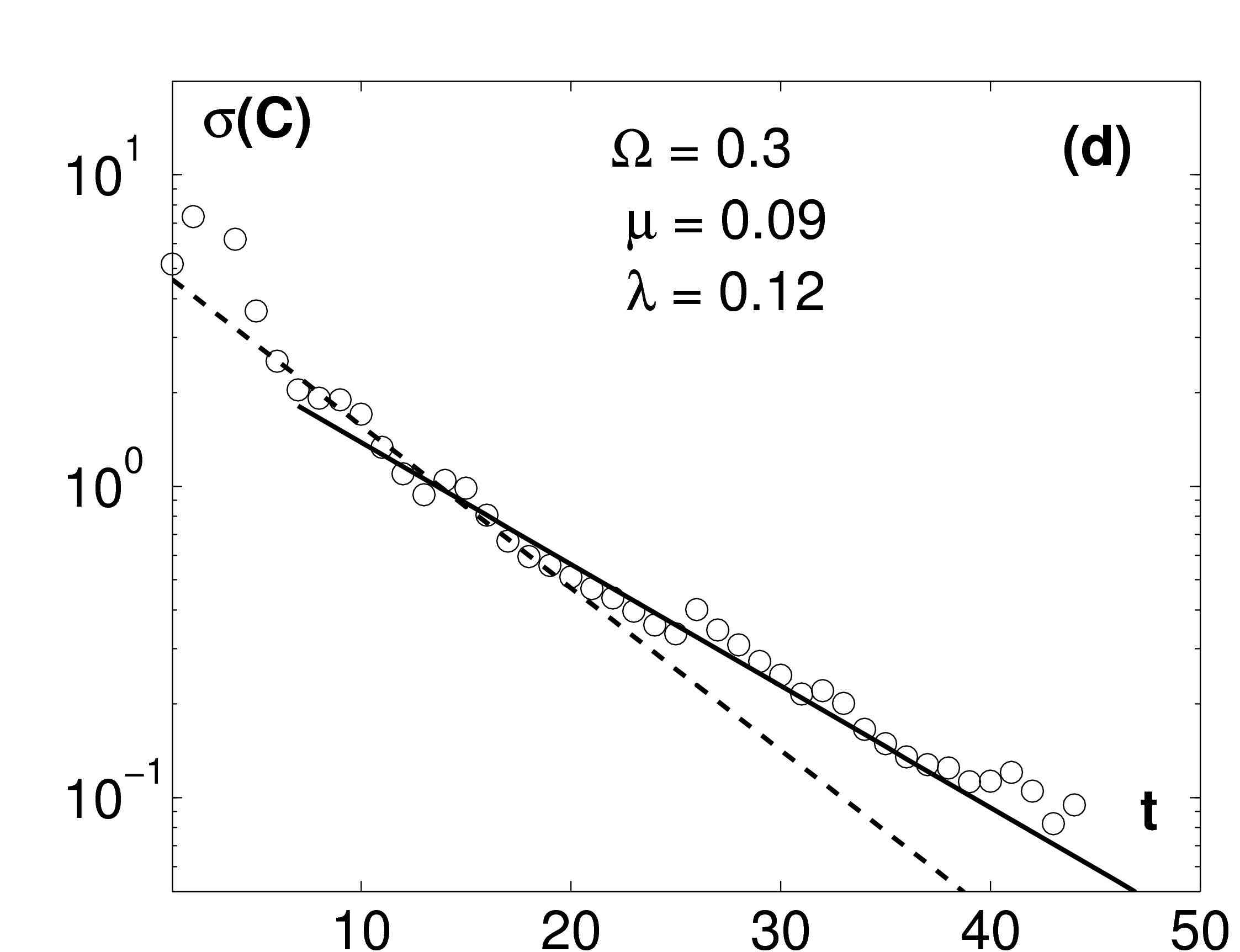
Figure 4: Evolution of the standard deviation $\sigma(C)$. (a) Sketch of the decay of $\sigma(C)$ according to the proposed scenario; (b)–(d) Actual decay measured in simulations of the figure-eight protocol, for three different wall velocities $\Omega$; the continuous (resp. dash) line shows an exponential decay with rate $\mu/2$ (resp. $\lambda/2$).

The fluctuations of the mixing pattern in Fig. 1(c) are dominated by the white strips injected most recently, as well as a few folds of strips injected previously—portions of the strips that are stretched but not folded reach $\ell$ faster. We therefore estimate that the total white area inside the bulk is the dominant contribution to the variance, and that it is proportional to $|{\dot{d\mkern 8.0mu}\mkern-8.0mu}{}(t)|\sim\exp(-\mu\,t/T)$. We observe indeed a decay of the variance at a rate close to $\mu$ for small values of $\Omega$ (Fig. 4(b–c)), consistent with a rate of mixing dominated by the rate of approach to the hyperbolic fixed point. The central mixing process is potentially more efficient ($\lambda>\mu$), but it is starved by the boundaries. When the rotation of the wall is increased so that $\mu$ becomes of the same order as $\lambda$ or greater, stretching in the bulk is as slow as that near the separatrix (or slower), so that the decay rate saturates at the same value $\lambda$ as during the initial decay phase.

In summary, we have proposed a design principle for mixing protocols that protect the chaotic mixing region from the slowdown due to no-slip walls. Creating a net rotation of the fluid in the vicinity of the wall results in a mixed phase space with a regular region that insulates the central chaotic region from the wall. In this case, we retrieve an exponential decay of scalar variance. For the case of a rotating vessel wall, rotating faster may increase the mixing efficiency. However, we have seen that the variance decay rate is always bounded by that of the bulk, and that when increasing $\Omega$ the total mixing region is smaller, so the influence of the separatrix is felt earlier. An understanging of this mechanism is a first step towards the design of efficient mixers. Depending on the application, it may for instance be appropriate to rotate the wall in such a way that $\mu(\Omega)\simeq\lambda$, to match the rate of stretching in the bulk to that near the outer hyperbolic point.

From a practical point of view, we note that for the epitrochoid protocol the rod itself generates the net rotation of the fluid elements, which qualitatively induces similar effects as above, but without the need for a rotating wall. Obviously, the biggest drawback of the design principle presented here—to insulate the chaotic region from the walls— is the presence of an unmixed region near the wall. But this may be unimportant in applications where one can selectively sample the mixture, for instance in pharmaceuticals. In any case, there is no other known practical way to avoid a wall-induced slowdown of the variance decay. Finally, from a more fundamental point of view it is intriguing that in all cases, including the epitrochoid, the decay rate inside the mixing region is always rather small, as compared for instance to that of a baker’s map. The origin of this slow mixing—the distribution of hyperbolic points, parabolic points, etc. Antonsen, Jr. et al. (1996); Balkovsky and Fouxon (1999); Thiffeault and Childress (2003); Gouillart et al. (2008)—is a key issue to investigate in the future.

The authors thank Matthew D. Finn for the use of his computer code for simulating viscous flows, as well as Cécile Gasquet and Vincent Padilla for technical assistance. J-LT was also partially supported by the Division of Mathematical Sciences of the US National Science Foundation, under grant DMS-0806821.

References

- Aref (1984) H. Aref, J. Fluid Mech. 143, 1 (1984).
- Ottino (1989) J. M. Ottino, The Kinematics of Mixing: Stretching, Chaos, and Transport (Cambridge University Press, Cambridge, U.K., 1989).
- Pikovsky and Popovych (2003) A. Pikovsky and O. Popovych, Europhys. Lett. 61, 625 (2003).
- groupedtheory (0000) M. Chertkov and V. Lebedev, Phys. Rev. Lett. 90, 034501 (2003); V. V. Lebedev and K. S. Turitsyn, Phys. Rev. E 69, 036301 (2004); H. Salman and P. H. Haynes, Phys. Fluids 19, 067101 (2007); O. Popovych, A. Pikovsky, and B. Eckhardt, Phys. Rev. E 75, 036308 (2007).
- groupednumerics (0000) S. C. Jana, G. Metcalfe, and J. M. Ottino, J. Fluid Mech. 269, 199 (1994); G. Boffetta, F. De Lillo, and A. Mazzino (2008), eprint arXiv:0811.4519; K. El Omari and Y. Le Guer, Comput. Therm. Sci. 1, 55 (2009).
- Gouillart et al. (2007) E. Gouillart, N. Kuncio, O. Dauchot, B. Dubrulle, S. Roux, and J.-L. Thiffeault, Phys. Rev. Lett. 99, 114501 (2007).
- Gouillart et al. (2008) E. Gouillart, O. Dauchot, B. Dubrulle, S. Roux, and J.-L. Thiffeault, Phys. Rev. E 78, 026211 (2008).
- Gouillart et al. (2009) E. Gouillart, O. Dauchot, J.-L. Thiffeault, and S. Roux, Phys. Fluids 21, 022603 (2009).
- Antonsen, Jr. et al. (1996) T. M. Antonsen, Jr., Z. Fan, E. Ott, and E. Garcia-Lopez, Phys. Fluids 8, 3094 (1996).
- Thiffeault and Childress (2003) J.-L. Thiffeault and S. Childress, Chaos 13, 502 (2003).
- Balkovsky and Fouxon (1999) E. Balkovsky and A. Fouxon, Phys. Rev. E 60, 4164 (1999).
- Pierrehumbert (1994) R. T. Pierrehumbert, Chaos Solitons Fractals 4, 1091 (1994).
- Fereday et al. (2002) D. R. Fereday, P. H. Haynes, A. Wonhas, and J. C. Vassilicos, Phys. Rev. E 65, 035301(R) (2002).
- Finn and Cox (2001) M. D. Finn and S. M. Cox, J. Eng. Math. 41, 75 (2001).
- Batchelor (1959) G. K. Batchelor, J. Fluid Mech. 5, 113 (1959).
- Thiffeault (2008) J.-L. Thiffeault, in Transport and Mixing in Geophysical Flows, edited by J. B. Weiss and A. Provenzale (Springer, Berlin, 2008), Lecture Notes in Physics 744, pp. 3–35, eprint arXiv:nlin/0502011.