Phenomenological model for the Drell-Yan process: Reexamined

Abstract

Drell-Yan pair production is investigated. We reexamine a model where the quark momentum fraction is defined as the ratio of the corresponding light cone components of the quark and parent nucleon in a naive parton-model approach. It is shown that results differ from the standard parton model. This is due to unphysical solutions for the momentum fractions within the naive approach which are not present in the standard parton model. In a calculation employing full quark kinematics, i.e. including primordial quark transverse momentum, these solutions also appear. A prescription is given to handle these solutions in order to avoid incorrect results. The impact of these solutions in the full kinematical approach is demonstrated and compared to the modified result.

I Introduction

The Drell-Yan (DY) process Drell:1970wh was first described in the 1970s and provides an important tool to access the distribution of partons inside the nucleon. While a lot of information can be gained from deep inelastic scattering Bjorken:1969ja , measurements of Drell-Yan events give complementary insights, especially about sea-quark distributions Alekhin:2006zm . This has sparked many studies of this process Halzen:1978rx ; Altarelli:1977kt ; Arnold:2008kf which are generally inspired by perturbative QCD (pQCD). A lot of experimental effort is being devoted to measurements of the DY process: In antiproton-proton collisions at $\overline{\textrm{P}}$ANDA (FAIR) Lutz:2009ff and PAX Barone:2005pu , in proton-proton collisions at RHIC Bunce:2000uv ; Bunce:2008aa , J-PARC Peng:2006aa ; Goto:2007aa ; Kumano:2008rt , IHEP Abramov:2005mk and JINR Sissakian:2008th and in pion-nucleon collisions at COMPASS Bradamante:1997mu ; Baum:1996yv . An overview of the experimental situation can be found in Reimer:2007iy . $\overline{\textrm{P}}$ANDA, for example, will allow measurements at hadron c.m. energies of a few GeV, where non-perturbative effects are expected to become more important. This highlights the need to model these effects in a phenomenological picture.

In addition the standard pQCD leading order (i.e. parton model) description does not fully describe the interesting observables. Invariant mass ($M$) spectra of the DY pair can only be accounted for by including an additional K-factor and transverse momentum ($p_{T}$) spectra are not accessible at all Gavin:1995ch . The latter can be partly cured by folding in a phenomenological Gaussian distribution for the transverse momentum, the width of which has to be fitted to data. However the absolute size of the cross sections is still underestimated D'Alesio:2004up . Next-to-leading-order (NLO) calculations improve the description in some aspects, but also bring about additional problems. The calculated invariant mass spectra come closer to the data and the $p_{T}$ spectra are comparable to data in the region $p_{T}\sim M$ Gavin:1995ch , but not for $p_{T}\rightarrow 0$ Halzen:1978rx . In fact the $p_{T}$-spectrum is divergent for $p_{T}\rightarrow 0$ in any fixed order of the strong coupling $\alpha_{s}$, due to large logarithmic corrections $\ln\left(M/p_{T}\right)$. These stem from soft gluon exchange and it is possible to remove these divergencies by an all-order resummation. However since $p_{T}$ is no longer a hard scale at $p_{T}\rightarrow 0$ additional non-pertubative (i.e. experimental) input is needed in these (and all other pQCD) approaches to describe the region of very small $p_{T}$ Collins:1984kg ; Davies:1984sp ; Fai:2003zc . Note here that the parton model (i.e. leading order) description is still a very useful starting point, e.g. for studying spin asymmetries in DY, since there NLO corrections appear to be rather small Shimizu:2005fp ; Barone:2005cr ; Martin:1997rz .

A phenomenological model that incorporates full transverse momentum dependent quark kinematics and which in addition allows for mass distributions of quarks was proposed to resolve these problems Linnyk:2004mt ; Linnyk:2005iw ; Linnyk:2006mv . The idea stems from the fact that in the usual collinear approach the parton momenta are confined to the beam direction, thus only one momentum component is different from zero. The other components, namely the transverse momentum and the mass of the parton, do not enter into the calculation of the partonic subprocess cross section. Since at finite energies these components might influence the cross section to some extent it is worthwhile to examine this influence in detail. However it turns out that in these works important physical constraints were not considered and thus incorrect results were obtained. In the current paper we examine these constraints in detail and present a prescription to properly account for them. Finally we compare the results of the treatment in Linnyk:2004mt ; Linnyk:2005iw ; Linnyk:2006mv with our corrected results. Since the mentioned problems already appear for the case without mass distributions for partons we restrict ourselves here to massless partons.

This paper is organized as follows: in Sec. II we compare the standard collinear parton model description for DY with an approach that defines the parton momentum fraction $x$ via light cone components. The latter approach will be a demonstration of the problems that appear in the calculation with the full kinematics. Section III contains two calculations in the full kinematical scheme, i.e. taking into account the full transverse momentum dependence of the partonic subprocess. The approach of Linnyk:2004mt ; Linnyk:2005iw ; Linnyk:2006mv is discussed in detail in Sec. III.2.1 and the technical details are given in the Appendix. Section III.2.2 then contains our calculation which respects the physical constraints laid out in Sec. II.2. The numerical results are presented in Sec. IV where we compare the two calculations of Sec. III quantitatively. Finally we present our conclusions in Sec. V.

In the following we present the conventions and notations used throughout this paper: It will turn out to be useful to write four-momenta using light-cone coordinates. We employ the following convention for general four-vectors $a$ and $b$

$$a^{+} =a_{0}+a_{z}\ ,$$ (1)

$$a^{-} =a_{0}-a_{z}\ ,$$ (2)

$$\vec{a}_{\perp} =\left(a_{x},a_{y}\right)\ ,$$ (3)

$$\Rightarrow a^{2} =a^{+}a^{-}-({\vec{a}}_{\perp})^{2}\ ,$$ (4)

$$\Rightarrow a\cdot b =\frac{1}{2}\left(a^{+}b^{-}+a^{-}b^{+}-2\,\vec{a}_{\perp}\cdot\vec{b}_{\perp}\right)\ .$$ (5)

We regard all particles as massless. We define the target nucleon to carry the four-momentum $P_{1}$ and the beam nucleon to carry the four-momentum $P_{2}$ (see fig. 1). In the hadron center-of-mass (c.m.) frame we choose the $z$-axis as the beam line and the beam (target) nucleon moves in the positive (negative) direction. Therefore the nucleon four-momenta read

$$P_{1} =\left(\frac{\sqrt{S}}{2},0,0,-\frac{\sqrt{S}}{2}\right)\ ,$$ (6)

$$P_{2} =\left(\frac{\sqrt{S}}{2},0,0,+\frac{\sqrt{S}}{2}\right)\ .$$ (7)

Note here that with a finite nucleon mass $P_{1}$ and $P_{2}$ would change. We have explicitly conducted the entire calculation with non-zero nucleon mass and convinced ourselves that it does not influence our arguments in Secs. II and III. Our results in Sec. IV would receive only a small correction, since we are looking at c.m. energies of $\sqrt{S}>27$ GeV. Thus, in this paper, we have put the nucleon mass to zero for the sake of simplicity and readability.

We denote the four-momentum of the parton in nucleon 1 (2) as $p_{1}$ ($p_{2}$). The on-shell condition in light-cone coordinates then reads

$$0=p_{i}^{2}=p_{i}^{+}p_{i}^{-}-({\vec{p}}_{i_{\perp}})^{2}\ .$$ (8)

The definition of the Feynman variable $x_{F}$ is Amsler:2008zzb

$$x_{F}=\frac{q_{z}}{(q_{z})_{\textrm{max}}}\ .$$ (9)

For the virtual photon in fig. 1 the maximal $q_{z}$ is derived by requiring the invariant mass of the undetected remnants to vanish and the photon to move collinearly to the nucleons:

$$\left(P_{1}+P_{2}-q\right)^{2} =X^{2}\overset{!}{=}0$$ (10)

$$\Rightarrow S+q^{2}-2\sqrt{S}\sqrt{q^{2}+(q_{z})_{\textrm{max}}^{2}} =0$$ (11)

$$\Rightarrow\frac{S-q^{2}}{2\sqrt{S}} =(q_{z})_{\textrm{max}}\ .$$ (12)

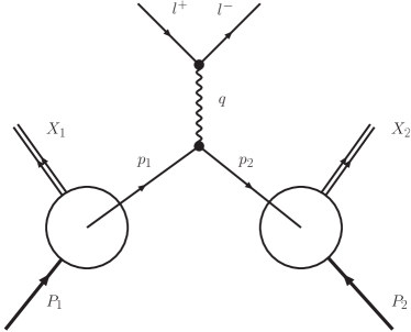
Figure 1: DY production in a nucleon-nucleon collision; $X_{1}$ and $X_{2}$ denote the nucleon remnants. See main text for details.

II Collinear approach

In this section we treat the interacting partons as collinear with their parent nucleons. We compare the standard textbook parton model with a naive approach which uses the light-cone component definition of the parton momentum fractions. It will turn out that in the latter case unphysical solutions appear that must be removed to be consistent with the standard parton model.

II.1 Standard parton model

The leading-order Drell-Yan total differential cross section in the standard parton model reads Drell:1970wh

$$\textrm{d}\sigma=\int_{0}^{1}\textrm{d}x_{1}\int_{0}^{1}\textrm{d}x_{2}\sum_{i}q_{i}^{2}\,f_{i}(x_{1},q^{2})\,f_{\bar{i}}(x_{2},q^{2})\,\textrm{d}\hat{\sigma}(x_{1},x_{2},q^{2})\ .$$ (13)

Here $x_{1}$ and $x_{2}$ are the momentum fractions carried by the annihilating partons inside the colliding nucleons:

$$p_{1} =x_{1}P_{1}\ ,$$ (14)

$$p_{2} =x_{2}P_{2}\ .$$ (15)

The sum runs over all quark flavors and antiflavors, $q_{i}$ denotes the electric charge of quark flavor $i$, the functions $f_{i}$ are parton distribution functions (PDFs) and $\textrm{d}\hat{\sigma}$ is the total differential cross section of the partonic subprocess,

$$\textrm{d}\hat{\sigma}=\frac{4\pi\alpha^{2}}{9q^{2}}\,\delta(M^{2}-q^{2})\,\delta^{(4)}(p_{1}+p_{2}-q)\,\textrm{d}^{4}q\,\textrm{d}M^{2}\ .$$ (16)

Here $q$ is the four-momentum of the virtual photon, $p_{1},p_{2}$ are the four-momenta of the partons (cf. fig. 1) and $\alpha\approx 1/137$ is the fine-structure constant.

Note that it becomes immediately clear from Eqs. (14) and (15) that the incoming partons move collinearly with the nucleons. According to Eq. (16) no transverse momentum can be generated for the virtual photon (and thus for the DY pair) in the leading-order process:

$${\vec{p}}_{1_{\perp}} ={\vec{p}}_{2_{\perp}}=0$$ (17)

$$\Rightarrow\delta^{(4)}(p_{1}+p_{2}-q) =\delta((p_{1}+p_{2})^{0}-q^{0})\,\delta^{(2)}({\vec{q}}_{\perp})$$

$$\,\times\delta((p_{1}+p_{2})^{z}-q^{z})\ .$$ (18)

The maximal information about the DY pair that can be gained from Eq. (13) is double differential. A common choice of variables is the squared invariant mass $M^{2}$ and Feynman’s $x_{F}$ of the virtual photon:

$$\frac{\textrm{d}\hat{\sigma}}{\textrm{d}M^{2}\ \textrm{d}x_{F}} =\int\textrm{d}^{4}q\frac{4\pi\alpha^{2}}{9q^{2}}\,\delta(M^{2}-q^{2})\,\delta^{(4)}(p_{1}+p_{2}-q)\,\delta\left(x_{F}-\frac{q_{z}}{(q_{z})_{\textrm{max}}}\right)=\frac{4\pi\alpha^{2}}{9M^{2}}\,\delta\left(M^{2}-(p_{1}+p_{2})^{2}\right)\,\delta\left(x_{F}-\frac{(p_{1}+p_{2})_{z}}{(q_{z})_{\textrm{max}}}\right)\ .$$ (19)

The two $\delta$-functions connect $x_{1}$ and $x_{2}$ with the chosen observables

$$M^{2} =2p_{1}p_{2}=x_{1}x_{2}S\ ,$$ (20)

$$x_{F} =+\frac{\sqrt{S}\,(x_{2}-x_{1})}{2(q_{z})_{\textrm{max}}}$$ (21)

with $(q_{z})_{\textrm{max}}=\frac{S-M^{2}}{2\sqrt{S}}$, cf. Eq. (12).

Solving for $x_{1}$ and $x_{2}$ yields

$$x_{1_{\pm}} =\frac{-(q_{z})_{\textrm{max}}\,x_{F}\pm\sqrt{\left((q_{z})_{\textrm{max}}\,x_{F}\right)^{2}+M^{2}}}{\sqrt{S}}$$

$$=\frac{-(q_{z})_{\textrm{max}}\,x_{F}\pm E_{\textrm{coll}}}{\sqrt{S}}\ ,$$ (22)

$$x_{2_{\pm}} =\frac{(q_{z})_{\textrm{max}}\,x_{F}\pm\sqrt{\left((q_{z})_{\textrm{max}}\,x_{F}\right)^{2}+M^{2}}}{\sqrt{S}}$$

$$=\frac{(q_{z})_{\textrm{max}}\,x_{F}\pm E_{\textrm{coll}}}{\sqrt{S}}\ ,$$ (23)

with the energy of the collinear DY-pair

$$E_{\textrm{coll}}=\sqrt{M^{2}+\left((q_{z})_{\textrm{max}}\,x_{F}\right)^{2}}\ .$$ (24)

However the lower solutions are always negative. Only the upper solutions are in the integration range of Eq. (13) and are physically meaningful. For the negative solutions the parton energies would be negative on account of Eqs. (14) and (15). The hadronic cross section then reads:

$$\frac{\textrm{d}\sigma}{\textrm{d}M^{2}\ \textrm{d}x_{F}} =\int_{0}^{1}\textrm{d}x_{1}\int_{0}^{1}\textrm{d}x_{2}\sum_{i}q_{i}^{2}f_{i}(x_{1},M^{2})\,f_{\bar{i}}(x_{2},M^{2})\,\frac{4\pi\alpha^{2}}{9M^{2}}\,\delta\left(M^{2}-(p_{1}+p_{2})^{2}\right)\,\delta\left(x_{F}-\frac{(p_{1}+p_{2})_{z}}{(q_{z})_{\textrm{max}}}\right)$$

$$=\int_{0}^{1}\textrm{d}x_{1}\int_{0}^{1}\textrm{d}x_{2}\sum_{i}q_{i}^{2}f_{i}(x_{1},M^{2})\,f_{\bar{i}}(x_{2},M^{2})\,\frac{4\pi\alpha^{2}}{9M^{2}}\,\frac{(q_{z})_{\textrm{max}}}{S\sqrt{(q_{z})^{2}_{\textrm{max}}x_{F}^{2}+M^{2}}}\delta(x_{1}-x_{1_{+}})\,\delta(x_{2}-x_{2_{+}})$$

$$=\sum_{i}q_{i}^{2}f_{i}(x_{1_{+}},M^{2})\,f_{\bar{i}}(x_{2_{+}},M^{2})\,\frac{4\pi\alpha^{2}}{9M^{2}}\,\frac{(q_{z})_{\textrm{max}}}{SE_{\textrm{coll}}}\ .$$ (25)

In this section we have presented the standard parton model solution for the leading-order DY cross section. The only quantities in this approach not determined by pQCD are the PDFs. These have to be obtained by fitting parametrizations to experimental data, mainly on deep inelastic scattering (DIS), but also on measurements of DY production itself Stirling:1900sj .

II.2 Naive parton model

In this section we work out the complete collinear kinematics using the definition of the parton momentum fraction as the ratio of light-cone components of the parton and the nucleon Jaffe:1985je . We show that there exist other solutions for the parton momentum fractions $x_{i}$ which are neglected in the standard parton model right from the start. These other solutions will turn out to be unphysical and are derived at this point only to provide insight into difficulties arising from a transverse-momentum dependent calculation as discussed in Sec. III.2.1.

The partons inside the nucleons carry some fraction of their parent hadron’s longitudinal momentum. Labeling the parton momentum inside nucleon $i$ with $p_{i}$ we can define these fractions as ratios of plus or minus components of the partons and the corresponding components of the nucleon momenta. In the Drell-Yan scaling limit ($S\rightarrow\infty$ and $M^{2}/S$ finite) $P_{1}^{-}=P_{2}^{+}=\sqrt{S}$ become the large components while all other components vanish. Note here that with a finite nucleon mass the large components would be modified and the small components would be nonzero. This however poses no problem for the following calculations, c.f. the discussion below Eqs. (6) and (7). We define

$$x_{1} =\frac{p_{1}^{-}}{P_{1}^{-}}=\frac{p_{1}^{-}}{\sqrt{S}}\ ,$$ (26)

$$\tilde{x}_{1} =\frac{p_{1}^{+}}{\sqrt{S}}\ ,$$ (27)

$$x_{2} =\frac{p_{2}^{+}}{P_{2}^{+}}=\frac{p_{2}^{+}}{\sqrt{S}}\ ,$$ (28)

$$\tilde{x}_{2} =\frac{p_{2}^{-}}{\sqrt{S}}\ .$$ (29)

Note that Eqs. (26) and (28) are standard definitions Jaffe:1985je . The tilde quantities in Eqs. (27) and (29) are introduced for later convenience. The kinematical constraints for these fractions are the on shell conditions

$$p_{1}^{2} =p_{1}^{+}p_{1}^{-}=0\Rightarrow x_{1}\tilde{x_{1}} =0\ ,$$ (30)

$$p_{2}^{2} =p_{2}^{+}p_{2}^{-}=0\Rightarrow x_{2}\tilde{x_{2}} =0\ ,$$ (31)

together with

$$M^{2}=(p_{1}+p_{2})^{2}=2p_{1}p_{2} =p_{1}^{+}p_{2}^{-}+p_{1}^{-}p_{2}^{+}$$

$$=\left(\tilde{x_{1}}\tilde{x_{2}}+x_{1}x_{2}\right)S$$ (32)

and

$$x_{F}=\frac{\left(p_{1}+p_{2}\right)_{z}}{(q_{z})_{\textrm{max}}} =\frac{1}{2(q_{z})_{\textrm{max}}}\left(p_{1}^{+}-p_{1}^{-}+p_{2}^{+}-p_{2}^{-}\right)$$

$$=\frac{\sqrt{S}}{2(q_{z})_{\textrm{max}}}\left(\tilde{x_{1}}-x_{1}+x_{2}-\tilde{x_{2}}\right)\ .$$ (33)

We will show now that the constraints in Eqs. (30)-(33) can be fulfilled by two different sets of momentum fractions $x_{i},\tilde{x_{i}}$. Equation (30) implies $\tilde{x_{1}}=0$ or $x_{1}=0$. If

$$\tilde{x_{1}} =0$$ (34)

$$\xRightarrow{\textrm{Eq. (\ref{invmass_cond})}}\frac{M^{2}}{S} =x_{1}x_{2}$$ (35)

$$\Rightarrow x_{1} \neq 0\neq x_{2}$$ (36)

$$\xRightarrow{\textrm{Eq. (\ref{onshell_cond2})}}\tilde{x_{2}} =0$$ (37)

$$\xRightarrow{\textrm{Eq. (\ref{feynx_cond})}}x_{F} =(x_{2}-x_{1})\frac{\sqrt{S}}{2(q_{z})_{\textrm{max}}}.$$ (38)

This is just the standard parton-model solution, Eqs. (20,21), as described in Sec. II.1. However there exists another solution, namely for $x_{1}=0$:

$$x_{1} =0$$ (39)

$$\xRightarrow{\textrm{Eq. (\ref{invmass_cond})}}\frac{M^{2}}{S} =\tilde{x_{1}}\tilde{x_{2}}$$ (40)

$$\Rightarrow\tilde{x_{1}} \neq 0\neq\tilde{x_{2}}$$ (41)

$$\xRightarrow{\textrm{Eq. (\ref{onshell_cond2})}}x_{2} =0$$ (42)

$$\xRightarrow{\textrm{Eq. (\ref{feynx_cond})}}x_{F} =(\tilde{x_{1}}-\tilde{x_{2}})\frac{\sqrt{S}}{2(q_{z})_{\textrm{max}}}\ .$$ (43)

Kinematically this second solution represents the (strange) case where each parton moves into the opposite direction of its respective parent nucleon. One can see this in the following example, where we choose $x_{F}=0$. Then we have

$$\tilde{x_{1}} =\tilde{x_{2}}=\frac{M}{\sqrt{S}}$$ (44)

$$\Rightarrow p_{1}^{z} =\frac{1}{2}\left(p_{1}^{+}-p_{1}^{-}\right)=\frac{1}{2}\sqrt{S}\tilde{x_{1}}=\frac{M}{2}$$ (45)

and analogously

$$p_{2}^{z}=-\frac{M}{2}\ .$$ (46)

Since nucleon 1 (2) moves into negative (positive) $z$-direction, cf. Eqs. (6) and (7), the partons here move exactly opposite. The parton momentum fractions $x_{i}$ (not $\tilde{x}_{i}$!) entering the PDFs in Sec. II.1 however are those of partons that move into the same direction as their parent nucleon. The second solution is thus physically not meaningful and it is discarded right away in the standard parton model approach.

The essential difference between the standard and the naive parton model is the following: In the (collinear) standard parton model all components of $p_{i}$ are fixed at once by $p_{i}=x_{i}P_{i}$. This automatically implies $\tilde{x}_{i}=0$. Such a procedure is without problems if one sticks to the collinear dynamics. In Sec. III below, however, we include primordial transverse momenta of the partons, i.e. we have to deviate from $p_{i}=x_{i}P_{i}$. The natural choice would be to define $x_{i}$ via one nucleon momentum component (the large one). This is exactly what we have done here for the collinear case. In the naive parton model $x_{i}$ and $\tilde{x}_{i}$, i.e. $p_{i}^{+}$ and $p_{i}^{-}$, are introduced as independent variables which are then constrained by the kinematical and onshell conditions (30)-(33). However in the Bjorken limit ($M,S\rightarrow\infty,M^{2}/S=\textrm{const}$) the parton momenta should behave like Arnold:2008kf

$$p_{1}^{-}=O(M),\ \ p_{1}^{+}=O(1/M),$$ (47)

$$p_{2}^{+}=O(M),\ \ p_{2}^{-}=O(1/M).$$ (48)

For $\tilde{x}_{i}\neq 0$ this power counting is not fulfilled, cf. Eqs. (27) and (29). Hence this solution corresponds to non-factorizing power suppressed corrections. Therefore in the naive parton model one falls into a trap by picking up this additional unphysical solution. The same happens for the more complicated case including primordial transverse momenta.

It is worth pointing out the connection between the two types of parton models (standard vs. naive) and QCD. There, e.g., the DY cross section formula emerges from factorisation. It turns out that in the Bjorken limit a PDF depends on one variable only Jaffe:1985je , which is encoded in $x_{i}$. In the final formula the energy-momentum relation, e.g., for the DY process takes the form $\delta(q-x_{1}P_{1}-x_{2}P_{2})$ which suggests the interpretation of $x_{i}P_{i}$ as the parton four-momentum. Thus the standard (collinear) parton model emerges from QCD and not the naive one.

Including in addition primordial transverse momenta one has to model the distributions of these momenta. However there is a constraint the chosen model has to obey: in the Bjorken limit one should come back to the standard parton model and not to the naive one since only the former emerges from QCD.

In the following we will point out how to modify the naive parton model such that one ends up with the standard parton model. This procedure will then be generalized to the case where primordial transverse momenta of the partons are included. In the naive parton model the hadronic cross section reads:

$$\frac{\textrm{d}\sigma_{\textrm{naive}}}{\textrm{d}M^{2}\ \textrm{d}x_{F}} =\int_{0}^{1}\textrm{d}x_{1}\int_{0}^{1}\textrm{d}x_{2}\sum_{i}q_{i}^{2}f_{i}(x_{1},M^{2})\,f_{\bar{i}}(x_{2},M^{2})\,\frac{4\pi\alpha^{2}}{9M^{2}}\,\delta\left(M^{2}-(p_{1}+p_{2})^{2}\right)\,\delta\left(x_{F}-\frac{(p_{1}+p_{2})_{z}}{(q_{z})_{\textrm{max}}}\right)$$

$$=\int_{0}^{1}\textrm{d}x_{1}\int_{0}^{1}\textrm{d}x_{2}\sum_{i}q_{i}^{2}f_{i}(x_{1},M^{2})\,f_{\bar{i}}(x_{2},M^{2})\,\frac{4\pi\alpha^{2}}{9M^{2}}\,\frac{2(q_{z})_{\textrm{max}}x_{1}x_{2}\left(\delta(x_{1}-x_{1_{+}})\,\delta(x_{2}-x_{2_{+}})+\delta(x_{1})\,\delta(x_{2})\right)}{S^{3/2}\left|(x_{1}x_{2}-\tilde{x}_{1}\tilde{x}_{2})(x_{1}+x_{2}+\tilde{x}_{1}+\tilde{x}_{2})\right|}$$ (49)

The unphysical second solution for the momentum fractions is represented by

$$\delta(x_{1})\,\delta(x_{2})\,x_{1}f_{i}(x_{1},M^{2})\,x_{2}f_{\bar{i}}(x_{2},M^{2})$$ (50)

in the last expression. Its contribution does not vanish since one obtains for large enough $M^{2}$ Gluck:1998xa

$$\underset{x\rightarrow 0}{\lim}\ \left(x\,f(x,M^{2})\right)>0\ .$$ (51)

We now introduce a notation which we will keep throughout this paper. Whenever we explicitly disregard unphysical solutions of the type of Eqs. (39)-(43) under an integral we denote this integral by $\fint$. Thus

$$\frac{\textrm{d}\sigma_{\textrm{naive}}}{\textrm{d}M^{2}\ \textrm{d}x_{F}} =\int_{0}^{1}\textrm{d}x_{1}\int_{0}^{1}\textrm{d}x_{2}\sum_{i}q_{i}^{2}f_{i}(x_{1},M^{2})\,f_{\bar{i}}(x_{2},M^{2})\,\frac{4\pi\alpha^{2}}{9M^{2}}\,\frac{2(q_{z})_{\textrm{max}}x_{1}x_{2}\left(\delta(x_{1}-x_{1_{+}})\,\delta(x_{2}-x_{2_{+}})+\delta(x_{1})\,\delta(x_{2})\right)}{S^{3/2}\left|(x_{1}x_{2}-\tilde{x}_{1}\tilde{x}_{2})(x_{1}+x_{2}+\tilde{x}_{1}+\tilde{x}_{2})\right|}$$ (52)

wheras

$$\frac{\textrm{d}\sigma}{\textrm{d}M^{2}\ \textrm{d}x_{F}} =\fint_{0}^{1}\textrm{d}x_{1}\fint_{0}^{1}\textrm{d}x_{2}\sum_{i}q_{i}^{2}f_{i}(x_{1},M^{2})\,f_{\bar{i}}(x_{2},M^{2})\,\frac{4\pi\alpha^{2}}{9M^{2}}\,\frac{2(q_{z})_{\textrm{max}}x_{1}x_{2}\left(\delta(x_{1}-x_{1_{+}})\,\delta(x_{2}-x_{2_{+}})+\delta(x_{1})\,\delta(x_{2})\right)}{S^{3/2}\left|(x_{1}x_{2}-\tilde{x}_{1}\tilde{x}_{2})(x_{1}+x_{2}+\tilde{x}_{1}+\tilde{x}_{2})\right|}$$

$$=\int_{0}^{1}\textrm{d}x_{1}\int_{0}^{1}\textrm{d}x_{2}\sum_{i}q_{i}^{2}f_{i}(x_{1},M^{2})\,f_{\bar{i}}(x_{2},M^{2})\,\frac{4\pi\alpha^{2}}{9M^{2}}\,\frac{2(q_{z})_{\textrm{max}}(x_{1}x_{2})\delta(x_{1}-x_{1_{+}})\,\delta(x_{2}-x_{2_{+}})}{S^{3/2}(x_{1}x_{2})(x_{1}+x_{2})}$$

$$=\sum_{i}q_{i}^{2}f_{i}(x_{1_{+}},M^{2})\,f_{\bar{i}}(x_{2_{+}},M^{2})\,\frac{4\pi\alpha^{2}}{9M^{2}}\,\frac{2(q_{z})_{\textrm{max}}}{S^{3/2}(x_{1_{+}}+x_{2_{+}})}$$

$$=\sum_{i}q_{i}^{2}f_{i}(x_{1_{+}},M^{2})\,f_{\bar{i}}(x_{2_{+}},M^{2})\,\frac{4\pi\alpha^{2}}{9M^{2}}\,\frac{(q_{z})_{\textrm{max}}}{SE_{\textrm{coll}}}\ .$$ (53)

Note that in the last expression we have recovered the standard parton-model result Eq. (25).

The main reason to present this naive approach in detail will become clear in the next section where we lift the simplification of a collinear movement of the partons with the nucleons.

III Full kinematics

The Bjorken limit and the corresponding infinite-momentum frame in which the standard parton model is well defined and derived from leading-order pQCD is an idealization of real experiments. There the nucleons will always move with some finite momentum and thus the partons inside the nucleons can have nonvanishing momentum components perpendicular to the beam line. The factorisation into hard (subprocess) and soft (PDFs) physics is proven in the collinear case at least for leading twist (expansion in $1/M$) in Collins:1989gx and in the transverse case at least for partons with low transverse momentum in Ji:2004xq .

III.1 Transverse-momentum distributions

For the calculation of the hadronic cross sections we will need transverse-momentum dependent parton distribution functions. We denote these by ${\tilde{f}}_{i}$. They are functions of the light-cone momentum fraction $x_{i}$, the transverse momentum ${\vec{p}}_{i_{\perp}}$ and the hard scale of the subprocess $q^{2}$. The general form of these functions however is unknown. Known rather well are the longitudinal PDFs. Since data of DY pair production are compatible with a Gaussian form of the $p_{T}$-spectrum up to a certain $p_{T}$ Webb:2003bj ; Webb:2003ps , we assume factorisation of the longitudinal and the transverse part of ${\tilde{f}}_{i}$ and make the following common ansatz Wang:1998ww ; Raufeisen:2002zp ; D'Alesio:2004up

$${\tilde{f}}_{i}(x_{i},{\vec{p}}_{i_{\perp}},q^{2})=f_{i}(x_{i},q^{2})\cdot f_{i_{\perp}}({\vec{p}}_{i_{\perp}})\ .$$ (54)

Here $f_{i}$ are the usual longitudinal PDFs and for $f_{i_{\perp}}$ we choose a Gaussian form,

$$f_{i_{\perp}}({\vec{p}}_{i_{\perp}})=\frac{1}{4\pi D^{2}}\exp\left(-\frac{({\vec{p}}_{i_{\perp}})^{2}}{4D^{2}}\right)\ .$$ (55)

The width parameter $D$ is connected to the average squared transverse momentum via

$$\left<({\vec{p}}_{i_{\perp}})^{2}\right>=\int\textrm{d}{\vec{p}}_{i_{\perp}}({\vec{p}}_{i_{\perp}})^{2}f_{i_{\perp}}({\vec{p}}_{i_{\perp}})=4D^{2}\$$ (56)

and it has to be fitted to the available data.

III.2 Cross section

Now we calculate the hadronic cross section $\textrm{d}\sigma$ taking into account the full kinematics. Since it is necessary to remove the unphysical solutions for the light-cone momentum fractions $x_{1}$ and $x_{2}$ which correspond to the ones found in Sec. II.2 for the collinear case, the calculation has to be conducted such that it is possible to disentangle the physical and the unphysical solution. First we will discuss in Sec. III.2.1 a straightforward calculation which however does not obey this requirement (the details of this calculation can be found in the Appendix). If one does not remove the unphysical solutions one produces unphysical results. This reveals a pitfall which the unawareness of this problem can create Linnyk:2004mt ; Linnyk:2005iw ; Linnyk:2006mv . In Sec. III.2.2 we will show how to properly remove the unphysical solutions as we did for the collinear case at the end of Sec. II.2.

In the transverse-momentum dependent approach the leading-order Drell-Yan total differential cross section reads D'Alesio:2004up

$$\textrm{d}\sigma=\int_{0}^{1}\textrm{d}x_{1}\int_{0}^{1}\textrm{d}x_{2}\int\textrm{d}{\vec{p}}_{1_{\perp}}\int\textrm{d}{\vec{p}}_{2_{\perp}}\sum_{i}q_{i}^{2}{\tilde{f}}_{i}(x_{1},{\vec{p}}_{1_{\perp}},q^{2}){\tilde{f}}_{\bar{i}}(x_{2},{\vec{p}}_{2_{\perp}},q^{2})\cdot\textrm{d}\hat{\sigma}(x_{1},{\vec{p}}_{1_{\perp}},x_{2},{\vec{p}}_{2_{\perp}},q^{2})\ .$$ (57)

In this approach the transverse momentum ($p_{T}=|{\vec{q}}_{\perp}|$) of the DY pair is accessible, since the annihilating quark and antiquark can have finite initial transverse momenta. Note that in the calculations of D'Alesio:2004up the partonic DY cross section $\textrm{d}\hat{\sigma}$ was taken in the collinear limit.

III.2.1 Naive calculation

In the naive approach the partonic triple-differential cross section reads:

$$\frac{\textrm{d}\hat{\sigma}_{\textrm{naive}}}{\textrm{d}M^{2}\ \textrm{d}x_{F}\textrm{d}p_{T}^{2}} =\int\textrm{d}^{4}q\frac{4\pi\alpha^{2}}{9q^{2}}\,\delta\left(M^{2}-q^{2}\right)\,\delta^{(4)}(p_{1}+p_{2}-q)\,\delta\left(x_{F}-\frac{q_{z}}{(q_{z})_{\textrm{max}}}\right)\delta\left(p_{T}^{2}-({\vec{q}}_{\perp})^{2}\right)$$

$$=\frac{4\pi\alpha^{2}}{9M^{2}}\,\delta\left(M^{2}-(p_{1}+p_{2})^{2}\right)\,\delta\left(x_{F}-\frac{(p_{1}+p_{2})_{z}}{(q_{z})_{\textrm{max}}}\right)\delta\left(p_{T}^{2}-({\vec{p}}_{1_{\perp}}+{\vec{p}}_{2_{\perp}})^{2}\right)\ .$$ (58)

Inserting Eq. (58) in Eq. (57) yields a multiple integral for the triple-differential cross section:

$$\frac{\textrm{d}\sigma_{\textrm{naive}}}{\textrm{d}M^{2}\ \textrm{d}x_{F}\textrm{d}p_{T}^{2}}=\int_{0}^{1}\textrm{d}x_{1}\int_{0}^{1}\textrm{d}x_{2}\int\textrm{d}{\vec{p}}_{1_{\perp}}\int\textrm{d}{\vec{p}}_{2_{\perp}} F(x_{1},{\vec{p}}_{1_{\perp}},x_{2},{\vec{p}}_{2_{\perp}},M^{2})\,$$

$$\times\ \delta\left(M^{2}-(p_{1}+p_{2})^{2}\right)\,\delta\left(x_{F}-\frac{(p_{1}+p_{2})_{z}}{(q_{z})_{\textrm{max}}}\right)\delta\left(p_{T}^{2}-({\vec{p}}_{1_{\perp}}+{\vec{p}}_{2_{\perp}})^{2}\right)\ .$$ (59)

All pieces which do not contain $\delta$-functions are collected in $F(...)$. The straightforward, but naive calculation of (59) was performed in Linnyk:2004mt ; Linnyk:2005iw ; Linnyk:2006mv . The details of this calculation can be found in the Appendix. Here we just want to point out the problems arising from this approach: the naive calculation with the full kinematics incorporates unphysical solutions for the momentum fractions $x_{i}$ which correspond to the unphysical solutions of the collinear case in Eqs. (39)-(43). However in the collinear kinematics it is quite clear that these solutions for $x_{i}$ cannot be the physically interesting ones, since they are just $x_{i}=0$ and the PDFs are divergent for small $x$ as one can conclude from (51). In the case of full kinematics the situation is similar, however due to the introduction of transverse quark momentum distributions the momentum fractions $x_{i}$ are smeared out around their collinear values. Nonetheless the unphysical solutions are still very close to zero and one picks up very large contributions of the diverging PDFs at such low $x$. This leads to a large enhancement of the cross section in the full kinematical approach and the data are now overestimated. The effect can be seen in Linnyk:2004mt ; Linnyk:2005iw ; Linnyk:2006mv and also in Sec. IV where we compare this naive approach and the correct calculation of the next section. In addition, in Sec. IV it will be shown that the $M$-dependence of the cross section is not reproduced in the naive approach.

III.2.2 Correct calculation

The analogue to Eq. (59) in the correct approach is (for the notation $\fint$ see Sec. II.2)

$$\frac{\textrm{d}\sigma}{\textrm{d}M^{2}\ \textrm{d}x_{F}\textrm{d}p_{T}^{2}}=\fint_{0}^{1}\textrm{d}x_{1}\fint_{0}^{1}\textrm{d}x_{2}\int\textrm{d}{\vec{p}}_{1_{\perp}}\int\textrm{d}{\vec{p}}_{2_{\perp}} F(x_{1},{\vec{p}}_{1_{\perp}},x_{2},{\vec{p}}_{2_{\perp}},M^{2})\,$$

$$\times\, \delta\left(M^{2}-(p_{1}+p_{2})^{2}\right)\,\delta\left(x_{F}-\frac{(p_{1}+p_{2})_{z}}{(q_{z})_{\textrm{max}}}\right)\,\delta\left(p_{T}^{2}-({\vec{p}}_{1_{\perp}}+{\vec{p}}_{2_{\perp}})^{2}\right)\ .$$ (60)

The $\delta$-functions in Eq. (60) must be worked out in a way that allows to discern physical and unphysical solutions for the momentum fractions $x_{i}$ in order to perform the $\fint$-integrations. For this aim it is useful to rewrite the parton momenta in terms of different variables:

$$q =p_{1}+p_{2}\ ,$$ (61)

$$k =\frac{1}{2}\left(p_{2}-p_{1}\right)\ .$$ (62)

Inverting the last two equations, we can use the on-shell conditions for the partons to get

$$0=p_{1}^{2}=\left(\frac{1}{2}q-k\right)^{2}=\frac{1}{4}q^{2}-k\cdot q+k^{2}$$ (63)

and

$$0=p_{2}^{2}=\left(\frac{1}{2}q+k\right)^{2}=\frac{1}{4}q^{2}+k\cdot q+k^{2}\ .$$ (64)

Adding and subtracting Eqs. (63) and (64) yields

$$k^{2} =-\frac{1}{4}M^{2}\ ,$$ (65)

$$k\cdot q =0\ .$$ (66)

Solving Eq. (65) for $k^{+}$ yields

$$k^{+}=\frac{\vec{k}_{\perp}^{2}-\frac{1}{4}M^{2}}{k^{-}}\ .$$ (67)

Inserting this result into Eq. (66) gives an equation quadratic in $k^{-}$:

$$0 =k^{+}q^{-}+k^{-}q^{+}-2\vec{k}_{\perp}\cdot\vec{q}_{\perp}$$

$$=\frac{\vec{k}_{\perp}^{2}-\frac{1}{4}M^{2}}{k^{-}}q^{-}+k^{-}q^{+}-2\vec{k}_{\perp}\cdot\vec{q}_{\perp}$$ (68)

$$\Rightarrow 0 =\left(k^{-}\right)^{2}q^{+}-2\vec{k}_{\perp}\cdot\vec{q}_{\perp}k^{-}+\left(\vec{k}_{\perp}^{2}-\frac{1}{4}M^{2}\right)q^{-}\ .$$ (69)

The solutions are

$$(k^{-})_{\pm}=\frac{\vec{k}_{\perp}\cdot\vec{q}_{\perp}}{q^{+}}\pm\sqrt{\left(\frac{\vec{k}_{\perp}\cdot\vec{q}_{\perp}}{q^{+}}\right)^{2}+\frac{q^{-}}{q^{+}}\left(\frac{1}{4}M^{2}-\vec{k}_{\perp}^{2}\right)}\ .$$ (70)

Inserting (70) into (68) gives the solutions for $k^{+}$:

$$(k^{+})_{\mp}=\frac{q^{+}}{q^{-}}\left(\frac{\vec{k}_{\perp}\cdot\vec{q}_{\perp}}{q^{+}}\mp\sqrt{\left(\frac{\vec{k}_{\perp}\cdot\vec{q}_{\perp}}{q^{+}}\right)^{2}+\frac{q^{-}}{q^{+}}\left(\frac{1}{4}M^{2}-\vec{k}_{\perp}^{2}\right)}\ \right)\ .$$ (71)

Rewriting now Eqs. (26) and (28) in terms of $q$ and $k$ we obtain the solutions for the parton momentum fractions:

$$(x_{1})_{\pm}=\frac{p_{1}^{-}}{\sqrt{S}}=\frac{1}{\sqrt{S}}\left(\frac{1}{2}q^{-}-(k^{-})_{\pm}\right)$$ (72)

and

$$(x_{2})_{\mp}=\frac{p_{2}^{+}}{\sqrt{S}}=\frac{1}{\sqrt{S}}\left(\frac{1}{2}q^{+}+(k^{+})_{\mp}\right)\ .$$ (73)

Since there are two solutions for $k^{-}$ and $k^{+}$, respectively, we also get two solutions for $x_{1}$, $x_{2}$. To determine which set of $x_{1},x_{2}$ and thus $k^{+},k^{-}$ has to be chosen we take the limit of zero parton transverse momentum. In this way one can make the connection to the collinear case (then $q^{2}\rightarrow q^{+}q^{-}=M^{2}$):

$$(k^{-})_{\pm} \rightarrow\pm\sqrt{\frac{q^{-}}{q^{+}}\frac{1}{4}M^{2}} =\pm\frac{q^{-}}{2}$$ (74)

$$(k^{+})_{\mp} \rightarrow\mp\sqrt{\frac{q^{+}}{q^{-}}\frac{1}{4}M^{2}} =\mp\frac{q^{+}}{2}$$ (75)

Inserting expressions (74) and (75) into (72) and (73) yields two solutions for the momentum fractions, just as in the collinear case in Sec. II.2:

$$(x_{1})_{\pm}\rightarrow\frac{1}{\sqrt{S}}\begin{cases}0\\ q^{-}\end{cases}$$ (76)

and

$$(x_{2})_{\mp}\rightarrow\frac{1}{\sqrt{S}}\begin{cases}0\\ q^{+}\end{cases}\ .$$ (77)

The lower solutions correspond to the standard parton model Eqs. (35), (38), since $x_{1}x_{2}=\frac{M^{2}}{S}$ and $x_{2}-x_{1}=\frac{2q_{z}}{\sqrt{S}}=x_{F}\frac{2(q_{z})_{\textrm{max}}}{\sqrt{S}}$. The upper solution then corresponds to the unphysical case $x_{1}=x_{2}=0$ and $\tilde{x}_{1}\neq 0\neq\tilde{x}_{2}$, see Eqs. (39)-(43).

This is the crucial point: to receive physically meaningful results from Eq. (60) one has to discard these upper solutions just as one does in the collinear case in Sec. II.2. This requires that the integrals in Eq. (60) are evaluated in the correct order, otherwise one cannot disentangle the two different solutions for $x_{1}$ and $x_{2}$. We will now present a calculation which respects this requirement. In Sec. IV we will show that the quantitative difference between this calculation and the calculation from Sec. III.2.1 is huge.

We begin by introducing several integrals over $\delta$-functions in Eq. (60). In this way we will transform the integration variables to the above chosen $q$ and $\vec{k}_{\perp}$:

$$\frac{\textrm{d}\sigma}{\textrm{d}M^{2}\ \textrm{d}x_{F}\textrm{d}p_{T}^{2}}= \fint_{0}^{1}\textrm{d}x_{1}\fint_{0}^{1}\textrm{d}x_{2}\int\textrm{d}{\vec{p}}_{1_{\perp}}\int\textrm{d}{\vec{p}}_{2_{\perp}}\int\textrm{d}{\vec{q}}_{\perp}\int\textrm{d}{\vec{k}}_{\perp}\int\textrm{d}q^{+}\int\textrm{d}q^{-}F(x_{1},{\vec{p}}_{1_{\perp}},x_{2},{\vec{p}}_{2_{\perp}},M^{2})$$

$$\times\delta(q^{+}-(p_{1}^{+}+p_{2}^{+}))\,\delta(q^{-}-(p_{1}^{-}+p_{2}^{-}))\,\delta^{(2)}({\vec{q}}_{\perp}-\left({\vec{p}}_{1_{\perp}}+{\vec{p}}_{2_{\perp}}\right))\,\delta^{(2)}({\vec{k}}_{\perp}-\frac{1}{2}\left({\vec{p}}_{1_{\perp}}-{\vec{p}}_{2_{\perp}}\right))$$

$$\times\delta\left(M^{2}-(p_{1}+p_{2})^{2}\right)\,\delta\left(x_{F}-\frac{(p_{1}+p_{2})_{z}}{(q_{z})_{\textrm{max}}}\right)\delta\left(p_{T}^{2}-({\vec{p}}_{1_{\perp}}+{\vec{p}}_{2_{\perp}})^{2}\right)\ .$$ (78)

First we perform

$$\int\textrm{d}{\vec{p}}_{1_{\perp}}\int\textrm{d}{\vec{p}}_{2_{\perp}}\delta^{(2)}\left({\vec{q}}_{\perp}-\left({\vec{p}}_{1_{\perp}}+{\vec{p}}_{2_{\perp}}\right)\right)\,\delta^{(2)}\left({\vec{k}}_{\perp}-\frac{1}{2}\left({\vec{p}}_{2_{\perp}}-{\vec{p}}_{1_{\perp}}\right)\right)=1\ .$$ (79)

Now we calculate the integral

$$\fint_{0}^{1}\textrm{d}x_{1}\fint_{0}^{1}\textrm{d}x_{2}\ \delta\left(q^{+}-(p_{1}^{+}+p_{2}^{+})\right)\,\delta\left(q^{-}-(p_{1}^{-}+p_{2}^{-})\right)\ .$$ (80)

According to Eqs. (70)-(73) the $\delta$-functions in the last expression have two possible solutions for each $p_{1}^{-}$ and $p_{2}^{+}$. However as explained above we now have to explicitly remove the unphysical solutions $(x_{1})_{+}$ and $(x_{2})_{-}$ , which are the ones corresponding to the upper sign in Eqs. (70) and (71):

$$\fint_{0}^{1}\textrm{d}x_{1}\fint_{0}^{1}\textrm{d}x_{2}\ \delta(q^{+}-(p_{1}^{+}+p_{2}^{+}))\,\delta(q^{-}-(p_{1}^{-}+p_{2}^{-}))$$

$$= \fint_{0}^{1}\textrm{d}x_{1}\fint_{0}^{1}\textrm{d}x_{2}\ \delta\left(q^{+}-\frac{\left(\frac{1}{2}{\vec{q}}_{\perp}-{\vec{k}}_{\perp}\right)^{2}}{x_{1}\sqrt{S}}-x_{2}\sqrt{S}\right)\,\delta\left(q^{-}-x_{1}\sqrt{S}-\frac{\left(\frac{1}{2}{\vec{q}}_{\perp}+{\vec{k}}_{\perp}\right)^{2}}{x_{2}\sqrt{S}}\right)$$

$$= \int_{0}^{1}\textrm{d}x_{1}\int_{0}^{1}\textrm{d}x_{2}\ \delta\left(q^{+}-\frac{\left(\frac{1}{2}{\vec{q}}_{\perp}-{\vec{k}}_{\perp}\right)^{2}}{(x_{1})_{-}\sqrt{S}}-(x_{2})_{+}\sqrt{S}\right)\,\delta\left(q^{-}-(x_{1})_{-}\sqrt{S}-\frac{\left(\frac{1}{2}{\vec{q}}_{\perp}+{\vec{k}}_{\perp}\right)^{2}}{(x_{2})_{+}\sqrt{S}}\right)$$

$$= \left|S-\frac{(\frac{1}{2}{\vec{q}}_{\perp}-{\vec{k}}_{\perp})^{2}(\frac{1}{2}{\vec{q}}_{\perp}+{\vec{k}}_{\perp})^{2}}{(x_{1})_{-}^{2}(x_{2})_{+}^{2}S}\right|^{-1}.$$ (81)

Using $\textrm{d}q^{+}\textrm{d}q^{-}=2\textrm{d}q_{0}\textrm{d}q_{z}$ we can evaluate some of the remaining integrals of Eq. (78) with the help of the $\delta$-functions:

$$\int\textrm{d}q^{+}\textrm{d}q^{-}\textrm{d}{\vec{q}}_{\perp}\delta\left(M^{2}-q^{2}\right)\,\delta\left(x_{F}-\frac{q_{z}}{(q_{z})_{\textrm{max}}}\right)\,\delta\left(p_{T}^{2}-({\vec{q}}_{\perp})^{2}\right)$$

$$=2 \int\textrm{d}q_{0}\textrm{d}{\vec{q}}_{\perp}\textrm{d}q_{z}\ \delta\left(M^{2}+({\vec{q}}_{\perp})^{2}+q_{z}^{2}-q_{0}^{2}\right)\,\delta\left(x_{F}-\frac{q_{z}}{(q_{z})_{\textrm{max}}}\right)\,\delta\left(p_{T}^{2}-({\vec{q}}_{\perp})^{2}\right)$$

$$=\ \ \frac{\pi\,(q_{z})_{\textrm{max}}}{E}$$ (82)

with $E=\sqrt{M^{2}+p_{T}^{2}+x_{F}^{2}(q_{z})_{\textrm{max}}^{2}}$ . Collecting the pieces, what remains of Eq. (78) is

$$\frac{\textrm{d}\sigma}{\textrm{d}M^{2}\ \textrm{d}x_{F}\textrm{d}p_{T}^{2}}=\int^{|{\vec{k}}_{\perp}|_{\textrm{max}}}\textrm{d}{\vec{k}}_{\perp}\frac{\pi\ (q_{z})_{\textrm{max}}}{E}\left|S-\frac{(\hat{\vec{p}}_{1_{\perp}})^{2}(\hat{\vec{p}}_{2_{\perp}})^{2}}{(x_{1})_{-}^{2}(x_{2})_{+}^{2}S}\right|^{-1}F((x_{1})_{-},\hat{\vec{p}}_{1_{\perp}},(x_{2})_{+},\hat{\vec{p}}_{2_{\perp}},M^{2})\ .$$ (83)

$(x_{1})_{-},\hat{\vec{p}}_{1_{\perp}},(x_{2})_{+}$ and $\hat{\vec{p}}_{2_{\perp}}$ are now fixed:

$$(x_{1})_{-} =\frac{1}{\sqrt{S}}\left(\frac{q^{-}}{2}-\frac{\vec{k}_{\perp}\cdot\vec{q}_{\perp}}{q^{+}}+\sqrt{\left(\frac{\vec{k}_{\perp}\cdot\vec{q}_{\perp}}{q^{+}}\right)^{2}+\frac{q^{-}}{q^{+}}\left(\frac{1}{4}M^{2}-\vec{k}_{\perp}^{2}\right)}\right)\ ,$$ (84)

$$(x_{2})_{+} =\frac{1}{\sqrt{S}}\left(\frac{q^{+}}{2}+\frac{\vec{k}_{\perp}\cdot\vec{q}_{\perp}}{q^{-}}+\sqrt{\left(\frac{\vec{k}_{\perp}\cdot\vec{q}_{\perp}}{q^{-}}\right)^{2}+\frac{q^{+}}{q^{-}}\left(\frac{1}{4}M^{2}-\vec{k}_{\perp}^{2}\right)}\right)\ ,$$ (85)

$$\hat{\vec{p}}_{1_{\perp}} =\frac{1}{2}{\vec{q}}_{\perp}-{\vec{k}}_{\perp}\ ,$$ (86)

$$\hat{\vec{p}}_{2_{\perp}} =\frac{1}{2}{\vec{q}}_{\perp}+{\vec{k}}_{\perp}$$ (87)

with

$$q^{+} =E+x_{F}(q_{z})_{\textrm{max}}\ ,$$ (88)

$$q^{-} =E-x_{F}(q_{z})_{\textrm{max}}\ ,$$ (89)

$$\left|{\vec{q}}_{\perp}\right| =p_{T}\ ,$$ (90)

$$\vec{k}_{\perp}\cdot\vec{q}_{\perp} =|\vec{k}_{\perp}|p_{T}\cos(\phi_{\perp})\ .$$ (91)

$|{\vec{k}}_{\perp}|_{\textrm{max}}$ is fixed by the condition that $(x_{1})_{-}$ and $(x_{2})_{+}$ must be real numbers:

$$({\vec{k}}_{\perp})^{2}<\frac{(M^{2}+p_{T}^{2})\frac{M^{2}}{4}}{M^{2}+p_{T}^{2}(1-\cos^{2}(\phi_{\perp}))}=({\vec{k}}_{\perp})^{2}_{\textrm{max}}\$$ (92)

We have convinced ourselves that this condition also guarantees that $0<(x_{1})_{-},(x_{2})_{+}<1$. Finally we arrive at the following expression:

$$\frac{\textrm{d}\sigma}{\textrm{d}M^{2}\ \textrm{d}x_{F}\textrm{d}p_{T}^{2}}=\int_{0}^{2\pi}\textrm{d}\phi_{\perp}\int_{0}^{({\vec{k}}_{\perp})^{2}_{\textrm{max}}}\frac{1}{2}\textrm{d}({\vec{k}}_{\perp})^{2}\frac{\pi\ (q_{z})_{\textrm{max}}}{E}\left|S-\frac{(\hat{\vec{p}}_{1_{\perp}})^{2}(\hat{\vec{p}}_{2_{\perp}})^{2}}{(x_{1})_{-}^{2}(x_{2})_{+}^{2}S}\right|^{-1}F((x_{1})_{-},\hat{\vec{p}}_{1_{\perp}},(x_{2})_{+},\hat{\vec{p}}_{2_{\perp}},M^{2})$$ (93)

with

$$F((x_{1})_{-},\hat{\vec{p}}_{1_{\perp}},(x_{2})_{+},\hat{\vec{p}}_{2_{\perp}},M^{2})=\sum_{i}q_{i}^{2}\,{\tilde{f}}_{i}\left((x_{1})_{-},\hat{\vec{p}}_{1_{\perp}},M^{2}\right)\,{\tilde{f}}_{\bar{i}}\left((x_{2})_{+},\hat{\vec{p}}_{2_{\perp}},M^{2}\right)\,\frac{4\pi\alpha^{2}}{9M^{2}}$$ (94)

and with ${\tilde{f}}_{i}$ defined in Eq. (54).

IV Results

In this section we present our quantitative results and compare the naive approach of Sec. III.2.1 and the correct approach of Sec. III.2.2. The data are from the NuSea Collaboration (E866) Webb:2003bj ; Webb:2003ps and from FNAL-E439 Smith:1981gv . For the collinear PDFs we used the GRV98 LO parametrization Gluck:1998xa available through CERN’s PDFLIB version 8.04 Plothow:2000aa .

IV.1 E866 – $p_{T}$-spectra

Experiment E866 measured continuum dimuon production in pp collisions at $S\approx 1500$ GeV². The triple-differential cross section as given by the E866 collaboration is

$$E\frac{\textrm{d}\sigma}{d^{3}p}\equiv\frac{2E}{\pi\sqrt{S}}\frac{\textrm{d}\sigma}{\textrm{d}x_{F}\textrm{d}p_{T}^{2}}$$ (95)

where an average over the azimuthal angle has been taken. The data are given in several bins of $M$, $x_{F}$ and $p_{T}$ and for every datapoint the average values $\left<M\right>$, $\left<x_{F}\right>$ and $\left<p_{T}\right>$ are given. Since our schemes provide Eqs. (115) and (93) we calculate the quantity of Eq. (95) for every datapoint using these averaged values and then perform a simple average in every $M^{2}$-bin:

$$\frac{2E}{\pi\sqrt{S}}\frac{\textrm{d}\sigma}{\textrm{d}x_{F}\textrm{d}p_{T}^{2}} \rightarrow\frac{2E}{\pi\sqrt{S}}\int_{M^{2}\textrm{-bin}}\frac{\textrm{d}\sigma}{\textrm{d}M^{2}\textrm{d}x_{F}\textrm{d}p_{T}^{2}}\textrm{d}M^{2}$$

$$\approx\frac{2E}{\pi\sqrt{S}}\Delta M^{2}\frac{\textrm{d}\sigma}{\textrm{d}M^{2}\textrm{d}x_{F}\textrm{d}p_{T}^{2}}\left(\left<M\right>,\left<x_{F}\right>,\left<p_{T}\right>\right)\ ,$$ (96)

where

$$E=\sqrt{\vrule height=10.0pt,width=0.0pt\left<M\right>^{2}+\left<p_{T}\right>^{2}+\left<x_{F}\right>^{2}\left<(q_{z})_{\textrm{max}}\right>^{2}}$$ (97)

and $\Delta M^{2}=M_{\textrm{max}}^{2}-M_{\textrm{min}}^{2}$ with $M_{\textrm{max}}$ ($M_{\textrm{min}}$) the upper (lower) limit of the bin.

We plot the results for the two different approaches in different $M$-bins in Fig. 2. Everywhere a value of $D=0.5$ GeV for the transverse momentum dispersion was chosen. The solid lines represent the correct approach. The shape of the spectra is described rather well which is due to the choice of the parameter $D$. However the absolute size is still underestimated and a factor $K\approx 1.75-2.0$ would be necessary to reproduce the height of the data. The naive approach is plotted with dashes. As already mentioned in Sec. III.2.1 the calculated cross section overestimates the data significantly. This can also be seen in Linnyk:2004mt ; Linnyk:2005iw ; Linnyk:2006mv . We note that the discrepancy between both approaches is about 1 order of magnitude and it becomes worse in the higher mass bin. This already indicates a wrong $M$ dependence of the naive approach.

Figure 2: $p_{T}$-spectrum obtained from the naive and the correct approach with $D=0.5$ GeV. Data are from E866 binned with
$4.2$ GeV $<M<5.2$ GeV and $7.2$ GeV $<M<8.7$ GeV,
$-0.05<x_{F}<0.15$. Only statistical errors are shown.

IV.2 E866 - $M$-spectrum

The double-differential cross section is given by the E866 collaboration as

$$M^{3}\frac{\textrm{d}\sigma}{\textrm{d}M\textrm{d}x_{F}}\ .$$ (98)

Again the data are given in several bins of $M$ and $x_{F}$ and for every datapoint the average values $\left<M\right>$ and $\left<x_{F}\right>$ are provided. Once more we start with Eqs. (115) and (93) and calculate the quantity of Eq. (98) by integrating over $p_{T}^{2}$ for every datapoint using these averaged values:

$$M^{3}\frac{\textrm{d}\sigma}{\textrm{d}M\textrm{d}x_{F}} \rightarrow\left<M\right>^{3}\int_{0}^{(p_{T})^{2}_{\textrm{max}}}\textrm{d}p_{T}^{2}\frac{\textrm{d}\sigma}{\textrm{d}M\textrm{d}x_{F}\textrm{d}p_{T}^{2}}=\left<M\right>^{3}\int_{0}^{(p_{T})^{2}_{\textrm{max}}}\textrm{d}p_{T}^{2}\ 2\left<M\right>\frac{\textrm{d}\sigma}{\textrm{d}M^{2}\textrm{d}x_{F}\textrm{d}p_{T}^{2}}\left(\left<M\right>,\left<x_{F}\right>\right)\ .$$ (99)

The maximal possible $p_{T}$ is determined by the kinematics.

$$P_{1}+P_{2} =q+X$$ (100)

$$\Rightarrow(P_{1}+P_{2}-q)^{2} =X^{2}=M_{R}^{2}$$ (101)

$$\Rightarrow S+M^{2}-M_{R}^{2} =2\ (P_{1}+P_{2})\ q$$

$$=2\sqrt{S}E$$

$$=2\sqrt{S}\sqrt{M^{2}+p_{T}^{2}+q_{z}^{2}}$$ (102)

$$\Rightarrow M^{2}+(p_{T})^{2}_{\textrm{max}}+q_{z}^{2} =E^{2}=\frac{(S+M^{2}-M_{R}^{2})^{2}}{4S}$$ (103)

$$\Rightarrow(p_{T})^{2}_{\textrm{max}} =\frac{(S+M^{2}-M_{R}^{2})^{2}}{4S}-M^{2}-q_{z}^{2}\ .$$ (104)

$M_{R}^{2}$ is the minimal invariant mass of the undetected remnants. We choose a value of $M_{R}=1.1$ GeV. Note that at c.m. energies of $\sqrt{S}\approx 27.4$ GeV (E439) and $\sqrt{S}\approx 38.8$ GeV (E866) we are not really sensitive to this value if it stays at or below a few GeV.

The results are plotted in Fig. 3. Again we use $D=0.5$ GeV. The solid line represents the correct approach, the long dashed line the naive one. For comparison the result of the standard (collinear) parton model is plotted with the short dashed line. Here the discrepancy between the naive and the correct approach is fully visible, since neither the slope nor the size of the $M$-spectrum is reproduced in the naive approach. Instead it gives almost a constant distribution. (Note here that this dataset is not shown or compared to calculations in Linnyk:2004mt ; Linnyk:2005iw ; Linnyk:2006mv .) The correct approach however describes the slope well and again a factor $K\approx 1.75-2.0$ is necessary to reach the absolute height of the data, as expected from the triple-differential results in the last section. Note that the result of the correct approach and the standard (collinear) parton model coincide.

Figure 3: $M$-spectrum obtained from naive and correct approach with $D=0.5$ and from the standard parton model. Note that the results from the latter two approaches are basically on top of each other. Data are from E866 binned with $-0.05<x_{F}<0.05$. Only statistical errors shown.

IV.3 E439 - $M$-spectrum

Experiment E439 measured dimuon production in pW collisions at $S\approx 750$ GeV². The double differential cross section

$$\frac{\textrm{d}\sigma}{\textrm{d}M\textrm{d}x_{F}^{\prime}}$$ (105)

has been given with

$$x_{F}^{\prime}=\frac{x_{F}}{1-\frac{M^{2}}{S}}$$ (106)

at a fixed $x_{F}^{\prime}=0.1$.

As before we begin with Eqs. (115) and (93) and calculate the quantity Eq. (105) by integrating over $p_{T}^{2}$ and performing a simple transformation from $x_{F}$ to $x_{F}^{\prime}$:

$$\frac{\textrm{d}\sigma}{\textrm{d}M\textrm{d}x_{F}^{\prime}} =\int_{0}^{(p_{T})^{2}_{\textrm{max}}}\textrm{d}p_{T}^{2}\frac{\textrm{d}\sigma}{\textrm{d}M\textrm{d}x_{F}^{\prime}\textrm{d}p_{T}^{2}}=\int_{0}^{(p_{T})^{2}_{\textrm{max}}}\textrm{d}p_{T}^{2}\ 2M\left(1-\frac{M^{2}}{S}\right)\frac{\textrm{d}\sigma}{\textrm{d}M^{2}\textrm{d}x_{F}\textrm{d}p_{T}^{2}}\left(M,x_{F}=x_{F}^{\prime}\left(1-\frac{M^{2}}{S}\right)\right)\ .$$ (107)

We plot the results in Fig. 4, the solid line represents the correct approach, the long dashed line the naive one. With the same parameter $D=0.5$ GeV as for the E866 case we find the same discrepancy between the two approaches. Again the correct approach reproduces the slope well and a factor $K\approx 1.6$ is required to fit the data, while the naive approach fails to describe the slope and absolute size of the cross section. Once more the result of the correct approach agrees well with the result of the standard parton model (short dashed).

Here we note the following: in Linnyk:2004mt ; Linnyk:2005iw ; Linnyk:2006mv the same data of experiment E439 are compared to calculations, however only to an approach including both initial quark transverse momentum and quark mass distributions. There it is found that the data can be described well without a K-factor. There is no comparison of E439 data with a transverse momentum dependent calculation with onshell quarks (i.e. what we call the naive approach) in Linnyk:2004mt ; Linnyk:2005iw ; Linnyk:2006mv . We acknowledge that the introduction of quark mass distributions lowers the cross section which somewhat compensates for the enhancement in the naive approach. Nonetheless we want to point out that even with additional smearing from the quark mass distributions the naive approach will always lead to the wrong $M$-dependence of the cross section. The reason is simply that the PDFs are probed in two areas: around the standard collinear parton model $x$, cf. Eq. (25), and in a region very close to $x=0$ where the PDFs behave very differently with $M$ and give much larger contributions than for the physical $x$, since the PDFs diverge rapidly for $x\rightarrow 0$. Thus we conclude that the agreement of the full calculation with the E439 data in Linnyk:2004mt ; Linnyk:2005iw ; Linnyk:2006mv must be erroneous.

Figure 4: $M$-spectrum obtained from naive and correct approach with $D=0.5$ and from the standard parton model. Note that the results from the latter two approaches are basically on top of each other. Data are from E439 with $x_{F}^{\prime}=0.1$.

V Conclusions

In this paper we reexamined a phenomenological model of Drell-Yan pair production Linnyk:2004mt ; Linnyk:2005iw ; Linnyk:2006mv . This model tried to describe the DY process in a parton model scheme which takes into account the full transverse parton kinematics in the hard subprocess. The aim was to reproduce the transverse momentum spectra of the DY pairs and in addition to reproduce the absolute size of the cross sections by introducing mass distributions of the partons.

We have shown that already in the first step of introducing full transverse kinematics important constraints were not considered. Unphysical solutions emerging in a (too) naive parton model contaminate the results. We have derived these constraints in the usual collinear approach and then made the connection to the more general case of full kinematics. It turned out that unawareness of these constraints can lead to a drastically different result of the calculations: while in Linnyk:2004mt ; Linnyk:2005iw ; Linnyk:2006mv the inclusion of the transverse kinematics in the subprocess leads to an overshoot of the cross section, our corrected approach shows no such behavior and instead nicely reproduces the standard parton model prediction for the invariant mass spectra and the low transverse momentum spectrum, however only up to a K factor. Additionally we find that the naive approach taken in Linnyk:2004mt ; Linnyk:2005iw ; Linnyk:2006mv produces a wrong $M$-dependence of the cross section. This is a crucial point since already the standard parton model reproduces the right slope of the $M$-spectrum. Therefore we conclude that the findings in Linnyk:2004mt ; Linnyk:2005iw ; Linnyk:2006mv that allow for a K factor free description of DY pair production are unwarranted.

Appendix A Naive calculation of the hadronic cross section with full kinematics

Rewriting the $\delta$-functions of Eq. (59) in terms of the integration variables yields

$$\delta\left(M^{2}-(p_{1}+p_{2})^{2}\right)\,\delta\left(x_{F}-\frac{(p_{1}+p_{2})_{z}}{(q_{z})_{\textrm{max}}}\right)\,\delta\left(p_{T}^{2}-({\vec{p}}_{1_{\perp}}+{\vec{p}}_{2_{\perp}})^{2}\right)$$

$$=\, \delta\left(M^{2}-p_{1}^{+}p_{2}^{-}-p_{1}^{-}p_{2}^{+}+2{\vec{p}}_{1_{\perp}}\cdot{\vec{p}}_{2_{\perp}}\right)\,\delta\left(x_{F}-\frac{p_{1}^{+}-p_{1}^{-}+p_{2}^{+}-p_{2}^{-}}{2(q_{z})_{\textrm{max}}}\right)\,\delta\left(p_{T}^{2}-({\vec{p}}_{1_{\perp}})^{2}-({\vec{p}}_{2_{\perp}})^{2}-2{\vec{p}}_{1_{\perp}}\cdot{\vec{p}}_{2_{\perp}}\right)$$

$$=\, \delta\left(M^{2}-\frac{({\vec{p}}_{1_{\perp}})^{2}}{p_{1}^{-}}\frac{({\vec{p}}_{2_{\perp}})^{2}}{p_{2}^{+}}-p_{1}^{-}p_{2}^{+}+p_{T}^{2}-({\vec{p}}_{1_{\perp}})^{2}-({\vec{p}}_{2_{\perp}})^{2}\right)\,\delta\left(x_{F}-\frac{\frac{({\vec{p}}_{1_{\perp}})^{2}}{p_{1}^{-}}-p_{1}^{-}+p_{2}^{+}-\frac{({\vec{p}}_{2_{\perp}})^{2}}{p_{2}^{+}}}{2(q_{z})_{\textrm{max}}}\right)$$

$$\times\delta\left(p_{T}^{2}-({\vec{p}}_{1_{\perp}})^{2}-({\vec{p}}_{2_{\perp}})^{2}-2{\vec{p}}_{1_{\perp}}\cdot{\vec{p}}_{2_{\perp}}\right)$$

$$=\, \delta\left(M^{2}-\frac{({\vec{p}}_{1_{\perp}})^{2}}{x_{1}\sqrt{S}}\frac{({\vec{p}}_{2_{\perp}})^{2}}{x_{2}\sqrt{S}}-x_{1}\sqrt{S}x_{2}\sqrt{S}+p_{T}^{2}-({\vec{p}}_{1_{\perp}})^{2}-({\vec{p}}_{2_{\perp}})^{2}\right)\,\delta\left(x_{F}-\frac{\frac{({\vec{p}}_{1_{\perp}})^{2}}{x_{1}\sqrt{S}}-x_{1}\sqrt{S}+x_{2}\sqrt{S}-\frac{({\vec{p}}_{2_{\perp}})^{2}}{x_{2}\sqrt{S}}}{2(q_{z})_{\textrm{max}}}\right)\,$$

$$\times\delta\left(p_{T}^{2}-({\vec{p}}_{1_{\perp}})^{2}-({\vec{p}}_{2_{\perp}})^{2}-2{\vec{p}}_{1_{\perp}}\cdot{\vec{p}}_{2_{\perp}}\right)\ .$$ (108)

Note here that if one puts all transverse momenta in Eq. (108) to zero the collinear relations (32,33) are recovered. Note also that the unphysical parts of Eqs. (32) and (33) are included here since

$$\tilde{x}_{1} =\frac{p_{1}^{+}}{\sqrt{S}}\rightarrow\frac{({\vec{p}}_{1_{\perp}})^{2}}{x_{1}\sqrt{S}}\ ,$$ (109)

$$\tilde{x}_{2} =\frac{p_{2}^{-}}{\sqrt{S}}\rightarrow\frac{({\vec{p}}_{2_{\perp}})^{2}}{x_{2}\sqrt{S}}\ .$$ (110)

Now using the first two $\delta$-functions of Eq. (108) we can obtain solutions for the squared transverse momenta:

$$\delta\left(M^{2}-\frac{({\vec{p}}_{1_{\perp}})^{2}}{x_{1}\sqrt{S}}\frac{({\vec{p}}_{2_{\perp}})^{2}}{x_{2}\sqrt{S}}-x_{1}\sqrt{S}x_{2}\sqrt{S}+p_{T}^{2}-({\vec{p}}_{1_{\perp}})^{2}-({\vec{p}}_{2_{\perp}})^{2}\right)\,\delta\left(x_{F}-\frac{\frac{({\vec{p}}_{1_{\perp}})^{2}}{x_{1}\sqrt{S}}-x_{1}\sqrt{S}+x_{2}\sqrt{S}-\frac{({\vec{p}}_{2_{\perp}})^{2}}{x_{2}\sqrt{S}}}{2(q_{z})_{\textrm{max}}}\right)$$

$$=\, (q_{z})_{\textrm{max}}\,\frac{x_{1}x_{2}S}{E}\,\delta\left(({\vec{p}}_{1_{\perp}})^{2}-\left(E-x_{2}\sqrt{S}+(q_{z})_{\textrm{max}}x_{F}\right)x_{1}\sqrt{S}\right)\,\delta\left(({\vec{p}}_{2_{\perp}})^{2}-\left(E-x_{1}\sqrt{S}-(q_{z})_{\textrm{max}}x_{F}\right)x_{2}\sqrt{S}\right)\ ,$$ (111)

with the energy of the virtual photon

$$E=\sqrt{M^{2}+p_{T}^{2}+(q_{z})^{2}_{\textrm{max}}x_{F}^{2}}\ .$$ (112)

We note that exactly at this point the physical and the unphysical solutions for the momentum fractions $x_{i}$ have been mixed up by rewriting the $\delta$-functions, since the unphysical solutions of Eqs. (109) and (110) have entered.

Transforming the transverse momentum integrals

$$\int\textrm{d}{\vec{p}}_{1_{\perp}}\int\textrm{d}{\vec{p}}_{2_{\perp}}=\int_{-\pi}^{\pi}\textrm{d}{\phi}_{1_{\perp}}\int_{0}^{2\pi}\textrm{d}{\phi}_{2_{\perp}}\int_{0}^{\infty}\frac{1}{2}\textrm{d}({\vec{p}}_{1_{\perp}})^{2}\int_{0}^{\infty}\frac{1}{2}\textrm{d}({\vec{p}}_{2_{\perp}})^{2}$$ (113)

we can rewrite the entire expression (59) in the following form:

$$\frac{\textrm{d}\sigma_{\textrm{naive}}}{\textrm{d}M^{2}\ \textrm{d}x_{F}\textrm{d}p_{T}^{2}}= \int_{0}^{1}\textrm{d}x_{1}\int_{0}^{1}\textrm{d}x_{2}\int_{-\pi}^{\pi}\textrm{d}{\phi}_{1_{\perp}}\int_{0}^{2\pi}\textrm{d}{\phi}_{2_{\perp}}\int_{0}^{\infty}\frac{1}{2}\textrm{d}({\vec{p}}_{1_{\perp}})^{2}\int_{0}^{\infty}\frac{1}{2}\textrm{d}({\vec{p}}_{2_{\perp}})^{2}$$

$$\times\, \frac{(q_{z})_{\textrm{max}}{x_{1}x_{2}S}}{E}\,\frac{F(x_{1},{\vec{p}}_{1_{\perp}},x_{2},{\vec{p}}_{2_{\perp}},q^{2})}{\sqrt{4({\vec{p}}_{1_{\perp}})^{2}({\vec{p}}_{2_{\perp}})^{2}-\left(p_{T}^{2}-({\vec{p}}_{1_{\perp}})^{2}-({\vec{p}}_{2_{\perp}})^{2}\right)^{2}}}$$

$$\times\, \delta\left(({\vec{p}}_{1_{\perp}})^{2}-\left(E-x_{2}\sqrt{S}+(q_{z})_{\textrm{max}}x_{F}\right)x_{1}\sqrt{S}\right)\,\delta\left(({\vec{p}}_{2_{\perp}})^{2}-\left(E-x_{1}\sqrt{S}-(q_{z})_{\textrm{max}}x_{F}\right)x_{2}\sqrt{S}\right)$$

$$\times\, \delta\left({\phi}_{1_{\perp}}-\arccos\left(\frac{p_{T}^{2}-\left({\vec{p}}_{1_{\perp}}\right)^{2}-\left({\vec{p}}_{2_{\perp}}\right)^{2}}{\sqrt{4\left({\vec{p}}_{1_{\perp}}\right)^{2}\left({\vec{p}}_{2_{\perp}}\right)^{2}}}\right)\right)\ .$$ (114)

Now all four integrations concerning the partons’ transverse momenta can be carried out, leaving a two-dimensional integral which must be calculated numerically:

$$\frac{\textrm{d}\sigma_{\textrm{naive}}}{\textrm{d}M^{2}\ \textrm{d}x_{F}\textrm{d}p_{T}^{2}}=\int\textrm{d}x_{1}\int\textrm{d}x_{2}\frac{\pi\,(q_{z})_{\textrm{max}}{x_{1}x_{2}S}}{E}\,\frac{F(x_{1},\hat{\vec{p}}_{1_{\perp}},x_{2},\hat{\vec{p}}_{2_{\perp}},q^{2})}{\sqrt{4\left(\hat{\vec{p}}_{1_{\perp}}\right)^{2}\left(\hat{\vec{p}}_{2_{\perp}}\right)^{2}-\left(p_{T}^{2}-\left(\hat{\vec{p}}_{1_{\perp}}\right)^{2}-\left(\hat{\vec{p}}_{2_{\perp}}\right)^{2}\right)^{2}}}\ .$$ (115)

$\left(\hat{\vec{p}}_{1_{\perp}}\right)^{2}$ and $\left(\hat{\vec{p}}_{2_{\perp}}\right)^{2}$ are given by the $\delta$-functions in Eq. (111) and the integration boundaries of $x_{1}$ and $x_{2}$ have to be chosen such that the requirements

$$(\hat{\vec{p}}_{1_{\perp}})^{2} >0\ ,$$ (116)

$$(\hat{\vec{p}}_{2_{\perp}})^{2} >0\ ,$$ (117)

$$4(\hat{\vec{p}}_{1_{\perp}})^{2}(\hat{\vec{p}}_{2_{\perp}})^{2}-\left(p_{T}^{2}-(\hat{\vec{p}}_{1_{\perp}})^{2}-(\hat{\vec{p}}_{2_{\perp}})^{2}\right)^{2} >0$$ (118)

are fulfilled. One finds

$$0<x_{1}<\frac{E-x_{F}(q_{z})_{\textrm{max}}}{\sqrt{S}}$$ (119)

and

$$\frac{x_{1}\sqrt{S}(M^{2}-p_{T}^{2})+p_{T}^{2}\,(E-x_{F}(q_{z})_{\textrm{max}})-2Mp_{T}\sqrt{x_{1}\sqrt{S}(E-x_{F}(q_{z})_{\textrm{max}}-x_{1}\sqrt{S})}}{\sqrt{S}(E-x_{F}(q_{z})_{\textrm{max}})^{2}}$$

$$<x_{2}<$$

$$\frac{x_{1}\sqrt{S}(M^{2}-p_{T}^{2})+p_{T}^{2}\,(E-x_{F}(q_{z})_{\textrm{max}})+2Mp_{T}\sqrt{x_{1}\sqrt{S}(E-x_{F}(q_{z})_{\textrm{max}}-x_{1}\sqrt{S})}}{\sqrt{S}(E-x_{F}(q_{z})_{\textrm{max}})^{2}}\ .$$ (120)