Transient dynamics of molecular devices under step-like pulse bias

Abstract

We report first principles investigation of time-dependent current of molecular devices under a step-like pulse. Our results show that although the switch-on time of the molecular device is comparable to the transit time, much longer time is needed to reach the steady state. In reaching the steady state the current is dominated by resonant states below Fermi level. The contribution of each resonant state to the current shows the damped oscillatory behavior with frequency equal to the bias of the step-like pulse and decay rate determined by the life time of the corresponding resonant state. We found that all the resonant states below Fermi level have to be included for accurate results. This indicates that going beyond wideband limit is essential for a quantitative analysis of transient dynamics of molecular devices.

Anticipating a variety of technological applications, molecular scale conductors and devices are the subject of increasingly more research in recently years. One of the most important issues of molecular electronics concerns the dynamic response of molecular devices to external parametersgross3 ; Zhu ; yip ; Maciejko ; diventra ; chen1 ; gross2 . For ac quantum transport in such small devices, atomic details and non-equilibrium physics must be taken into account. So, in principle, one should use the theory of non-equilibrium Green’s function (NEGF)Jauho2 coupled with the time-dependent density functional theory (TDDFT)gross1 to study the time-dependent transport of molecular devices. Practically, it is very difficult to implement it at present stage due to the huge computational cost. One possible way to overcome this problem is to use the adiabatic approximation, an approach widely used in mesoscopic physics. In this approach, one starts from a steady-state Hamiltonian and adds the time dependent electric field adiabatically. This is a reasonable approximation since most of the time the applied electric field is much smaller than the electrostatic field inside the scattering region. In addition, it has been shown numericallychen1 that dc transport properties such as I-V curve obtained from the equation of motion method coupled with TDDFT agrees with that obtained by the method of NEGF coupled with the density functional theory (DFT)mcdcal ; brand . Hence, under the adiabatic approximation, one could replace TDDFT by DFT and use the NEGF+DFT scheme to calculate ac transport properties of molecular devices.

We consider a system that consists of a scattering region coupled to two leads with the external time dependent pulse bias potential $v_{\alpha}(t)$. The time-dependent current for a step-like pulse has been derived exactly going beyond the wide-band limit by Maciejko et alMaciejko . Since the general expression for the current involves triple integrations, it is extremely difficult if not impossible to calculate the time-dependent current for real systems like molecular devices. In this regard, approximation has to be made in order to carry out time-dependent simulations of molecular devices. We note that the simplest approximation is the so called wide-band approximation where self-energies $\Sigma^{r,a}$ are assumed to be independent of energy.Jauho1 Indeed, if such an approximation is used, i.e., $\Sigma^{r}=-i\Gamma/2$, one recovers the expression of transient current first obtained by Wingreen et alJauho1 . However, there are two problems when applying this approximation to investigate the dynamics of molecular devices. First of all, one assumes implicitly that the contribution to the transient current is dominated by only one resonant level with a constant linewidth function $\Gamma$ in the system in such an approximation. As we shall show below that this is not a good assumption in first principles investigation of the dynamics of molecular devices because there could be several resonant levels that significantly contribute to the transient current in molecular devices. Secondly, in the steady state limits at $t=0$ and $=\infty$ the wide-band limit can not reproduce the correct dc I-V curve obtained from first principles. By assuming the wide-band limit one can get a very different current that depends on the choice of $\Gamma$. In this paper, we propose an approximate formula of transient current that is suitable for numerical calculation for real molecular devices. Our scheme is an approximation of the exact solution of Maciejko et alMaciejko while keeping essential physics of dynamic systems. Using this scheme, we have calculated the transient current for several molecular devices. We found that all the resonant states below Fermi level contribute to the transient current. Each resonant state gives a damped oscillatory behavior with frequency equal to the bias of pulse and decay rate equal to its life time. Because of sharp resonances, it takes much longer time for the current to relax to the equilibrium value. For instance, for a $Al-C_{4}-Al$ structure with a transit time of $L/v_{F}=1.3fs$ the relaxation time is about 50fs. For a CNT-DTB-CNT structure with a transit time of 1fs, however, the relaxation time can reach several ps due to the resonant state with long lifetime. Our results indicated that going beyond wide-band limit is crucial for accurate predictions of dynamic response of molecular devices.

From Ref.Jauho1, ; Maciejko, , the current is expressed as ($\hbar=q=1$),

$$J_{\alpha}(t)=2{\rm Re}\int\frac{d\epsilon}{2\pi}{\rm Tr}[{\cal J}_{\alpha}(t,\epsilon)]$$ (1)

where

$${\cal J}_{\alpha}(t,\epsilon)=A_{\alpha}(t,\epsilon)\Sigma^{<,0}_{\alpha}(\epsilon)+\sum_{\beta}A_{\beta}(t,\epsilon)\Sigma^{<,0}_{\beta}(\epsilon)F_{\beta\alpha}(t,\epsilon)$$ (2)

where $\Sigma^{<,0}$ and $\Sigma^{a,0}$ are equilibrium self-energies and $A_{\alpha}(t,\epsilon)$ and $F_{\beta\alpha}(t,\epsilon)$ have different definitions for upward and downward pulses (see Ref.Maciejko, for details). In the absence of ac bias, $A_{\alpha}(t,\epsilon)$ is just the Fourier transform of retarded Green’s function. As discussed in Ref.Jauho2, that the first term in Eq.(2) corresponds to the current flowing into the central scattering region from lead $\alpha$ while the second term corresponds to the current flowing out from the central region into lead $\alpha$. From Eq.(1) we see that in order to calculate the transient current for a pulse bias we need to include the states with energy from $-\infty$ to the Fermi energy. This is very different from dc case where only the states with energy in the range $v_{L}-v_{R}$ about Fermi level contribute. Physically, this can be understood as follows. For ac transport with a sinusoidal bias $\cos(\omega t)$, the photon assisted tunnelling is significant only for the first a few sidebandsJauho2 . The step-like pulse can be expanded in terms of sinusoidal bias with continuous distribution of frequencies and each sinusoidal bias generates a photon sideband that facilitates the photon assisted tunnelling. Hence we expect that all the resonant states below Fermi level should be included and carefully examined in the calculation of transient current. Note that Eq.(1) and (2) are exact expressions with $A_{\alpha}(t,\epsilon)$ and $F_{\beta\alpha}(t,\epsilon)$ given in Ref.Maciejko, . Our approximation is made on $A_{\alpha}(t,\epsilon)$ and $F_{\beta\alpha}(t,\epsilon)$. For the upward pulse, $A_{\alpha}(t,\epsilon)$ and $F_{\beta\alpha}(t,\epsilon)$ are given by the following ansatz,

$$A^{u}_{\alpha}(t,\epsilon)=A^{u}_{1\alpha}(t,\epsilon)+A^{u}_{2\alpha}(t,\epsilon)$$ (3)

with

$$A^{u}_{1\alpha}(t,\epsilon) = \int\frac{dE}{2\pi i}\frac{e^{i(\epsilon-E+v_{\alpha})t}}{E-\epsilon-i0^{+}}~{}{\bar{G}}^{r}_{0}(E,\epsilon)$$

$$A^{u}_{2\alpha}(t,\epsilon) = \int\frac{dE}{2\pi i}\frac{1-e^{i(\epsilon-E+v_{\alpha})t}}{E-\epsilon-v_{\alpha}-i0^{+}}~{}{\bar{G}}^{r}_{\alpha}(E,\epsilon)$$ (4)

and

$$[F^{u}_{\beta\alpha}(t,\epsilon)]^{\dagger}=\Sigma^{r,0}_{\alpha}(\epsilon)A^{u}_{1\beta}+\Sigma^{r,0}_{\alpha}(\epsilon-v_{\alpha}+v_{\beta})A^{u}_{2\beta}$$ (5)

where

$${\bar{G}}^{r}_{0}(E,\epsilon)=1/[E-H-U_{eq}-\Sigma^{r,0}_{~{}}(\epsilon)]$$ (6)

$${\bar{G}}^{r}_{\alpha}(E,\epsilon)=1/[E-H-U-\sum_{\beta}\Sigma^{r,0}_{\beta}(\epsilon+v_{\alpha}-v_{\beta})]$$ (7)

with $U_{eq}$ and $U$ are, respectively, the equilibrium Coulomb potential and dc Coulomb potential at bias $v_{L}-v_{R}$. As will be illustrated in the examples given below this ansatz can be easily implemented to calculate the transient current for real molecular devices. Importantly, the results obtained from the ansatz captured essential physics of molecular devices. We wish to emphasize that our ansatz goes beyond the wide-band limit. It agrees with the expression of time-dependent current obtained by Wingreen et al in the wide-band limitJauho1 and produces correct limits at $t=0$ and $t\rightarrow\infty$.

Note that ${\bar{G}}^{r}_{0}(E,\epsilon)$ and ${\bar{G}}^{r}_{\alpha}(E,\epsilon)$ are different from the usual definition of Green’s functions, they allow us to perform contour integration over energy $E$ in Eq.(4) and (5) by closing a contour with an infinite radius semicircle at lower half plane. For a constant $\epsilon$, we have the following eigen equations

$$\left(H+U_{eq}+\Sigma^{r,0}(\epsilon)\right)|\psi^{0}_{n}\rangle = \epsilon^{0}_{n}|\psi^{0}_{n}\rangle$$

$$\left(H+U_{eq}+\Sigma^{a,0}(\epsilon)\right)|\varphi^{0}_{n}\rangle = \epsilon^{0*}_{n}|\varphi^{0}_{n}\rangle.$$ (8)

Expanding ${\bar{G}}^{r}_{0}(E,\epsilon)$ in terms of its eigen functions $|\psi^{0}_{n}\rangle$ and $|\phi^{0}_{n}\rangle$, we havefoot1

$${\bar{G}}^{r}_{0}(E,\epsilon)=\sum_{n}|\psi^{0}_{n}\rangle\langle\phi^{0}_{n}|/(E-\epsilon^{0}_{n}+i0^{+}).$$ (9)

With similar expression for ${\bar{G}}^{r}_{\alpha}(E,\epsilon)$, Eq.(4) can be written asfoot10

$$A^{u}_{1\alpha} = \sum_{n}\frac{e^{i(\epsilon-\epsilon^{0}_{n}+v_{\alpha})t}}{\epsilon-\epsilon^{0}_{n}+i0^{+}}|\psi^{0}_{n}\rangle\langle\phi^{0}_{n}|$$

$$A^{u}_{2\alpha} = \sum_{n}\frac{1-e^{i(\epsilon-\epsilon_{n}+v_{\alpha})t}}{\epsilon-\epsilon_{n}+v_{\alpha}+i0^{+}}|\psi_{n}\rangle\langle\phi_{n}|.$$ (10)

Now we show that our formalism gives the correct limits. At $t=0$ we have $A^{u}_{\alpha}(t,\epsilon)=G^{r}_{0}(\epsilon)$ and $F^{u}_{\beta\alpha}(t,\epsilon)=G^{a}_{0}(\epsilon)\Sigma^{a,0}_{\alpha}(\epsilon)$ with $G^{r}_{0}(\epsilon)$ the equilibrium Green’s function. This shows that the current from Eq.(2) is zero. Since all the poles $\epsilon^{0}_{n}$ and $\epsilon_{n}$ in Eq.(10) are on the lower half plane, at $t\rightarrow\infty$ we have $A^{u}_{\alpha}=G^{r}(\epsilon+v_{\alpha})$ and $F^{u}_{\beta\alpha}=G^{a}(\epsilon+v_{\beta})\Sigma^{a,0}_{\alpha}(\epsilon+v_{\beta}-v_{\alpha})$ where $G^{r}(\epsilon)$ is the Green’s function with dc bias $v_{\alpha}$ at $t\rightarrow\infty$. Substituting expressions of $A^{u}_{\alpha}$ and $F^{u}_{\beta\alpha}$ into Eq.(1), it gives the same dc current at the bias $v_{L}-v_{R}$. So far, we have discussed the ac conduction current $J_{\alpha}(t)$ under pulse-like bias. The displacement current $J_{\alpha}^{d}$ due to the charge pileup $dQ/dt$ inside the scattering region can be included using the method of current partitionbuttiker4 ; wbg : $J^{d}_{\alpha}=-(J_{L}+J_{R})/2$, so that the the total current is given by $I_{L}=(J_{L}-J_{R})/2$.Jauho2

With the formalism established, we now proceed to calculate the dynamic response of molecular devices. We have used the first principle quantum transport package ${\rm MatDcal}$.mcdcal To calculate the transient current for step-like pulse, we need to go through the following steps: (1). calculate two potential landscapes using NEGF-DFT package: the equilibrium potential $U_{eq}$ at $t=0$ and the dc potential $U$ at $t=\infty$. (2). With $U_{eq}$ and $U$ obtained, one solves eigenvalue problem using Eq.(8) and its counterpart for $U$, then find $A^{u}_{1\alpha}$ and $A^{u}_{2\alpha}$ from Eq.(10), and finally $A^{u}_{\alpha}$ and $F^{u}_{\beta\alpha}$ can be calculated from Eq.(3) and (5).

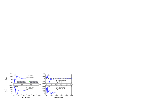
Figure 1: (color online) Transient current of $Al-C_{4}-Al$ structure at different bias $v_{L}=0.001,0.003,0.01,0.03au$. The solid line shows the transient current and the dotted line is the dc current $I_{dc}$ at bias $v_{L}-v_{R}=2v_{L}$. Inset of Fig.1a: schematic plot of the $Al-C_{4}-Al$ structure.

Inset of Fig.1a shows the structure of $Al-C_{4}-Al$ where $Al$ leads are along (100) direction. The nearest distance between $Al$ leads and the carbon chain is 3.781$au$ and the distance of C-C bond is 2.5$au$.($1au=0.529\AA$). Fig.1 shows the total transient currents $I_{L}(t)$ of the $Al-C_{4}-Al$ structure with various voltages $v_{L}(t)=-v_{R}(t)$. Following observations are in order. First of all, for all bias voltages the transient currents reached the correct limits at $t=0$ and $t=\infty$. Secondly, we see that once step-like voltage is turned on in the lead, currents oscillate rapidly with large amplitude in the first a few fs and then gradually approach to the steady-state values ($I_{dc}$ shown in the figure). In the first 10 to 30 fs, the current is much larger than that of the steady state value which agrees with the results obtained using first principle calculation with wide-band limitchen1 . For Fig.1a, the relaxation time (time to reach to steady state) is roughly 150 fs and for Fig.1b-1d the relaxation time is about 50fs. In addition, the switch-on time (the time to reach the maximum current) for the $Al-C_{4}-Al$ structure does not depend on the bias voltages. The typical switch-on time is about 2fs for applied bias voltage $v_{L}$ ranging from $0.001au$ to $0.01au$ $(1au=27.2V)$. For Al leads, the Fermi velocity is about $2\times 10^{6}$ m/s which corresponds to a transit time of 1.3 fs for the $Al-C_{4}-Al$ structure whose size is about $L=47$ $au$. Thirdly, we observe that the dc limit $I_{dc}$ at $v_{L}=0.01au$ is larger than that at $v_{L}=0.03au$. This is due to the appearance of the negative differential resistance at about $v_{L}=0.0075au$. Finally, there are several timescales characterizing the dynamic response of the molecular device. This can be seen clearly from Fig.1d that after 10 fs, the system shows a damped oscillation similar to the charging process of a classical RLC circuit. We will discuss this kind of oscillation in detail in the second example.

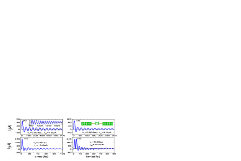
Figure 2: (color online) Transient current of CNT-DTB-CNT structure at different bias $v_{L}=0.001,0.003,0.01,0.02au$. The solid line shows the transient current and the dotted line is the dc current at bias $v_{L}-v_{R}=2v_{L}$. Inset of Fig.2b: schematic plot of the CNT-Di-thiol benzene-CNT structure.

As a second example, we study the transient current for di-thiol-benzene molecule (DTB) in contact with two (3,3) carbon nanotube (CNT) leads (see inset of Fig.2b). The structure is relaxed with the distance between the S atom and the nearest C atom equal to 2.73$au$ and the bond length of C-C being 3.61$au$. Fig.2 shows the transient current for different upward pulse biases. We see that for small bias $v_{L}=0.001au$, the current drops quickly in first 50 fs and then oscillates with much slower decay rate. It is found that the oscillatory part of the transient current is dominated by $\cos(2v_{L}t)$ which remains valid for the transient current at other biases $v_{L}$ shown in Fig.2b to Fig.2d. For instance, this gives the distance between adjacent peaks $\tau_{0}=76fs$ in Fig.2a when $v_{L}=0.001au$. With $1au=0.00242fs$, we obtain $\tau_{0}=\pi/v_{L}$. Different from the $Al-C_{4}-Al$ structure, it takes much longer time for the system to reach the equilibrium current $I_{L}(\infty)=1.5\mu A$ (after 5000fs the current is about $1.7\mu A$). From Fig.2a-2d, we conclude that the relaxation time is several ps.

Physically, this can be understood from the transmission coefficient $T(E)$. Fig.3 depicts $T(E)$ vs energy ranging from the transmission threshold to Fermi energy. We have scanned 100,000 energy points in order to resolve sharp resonant peaks labelled in Fig.3. In our calculation, 100 energy points were used for each sharp resonant peak (total 3000 energy points used) to converge the integration over $\epsilon$, i.e., $\int d\epsilon{\rm Tr}[{\cal J}_{\alpha}(t,\epsilon)]$ in Eq.(1). Since these sharp resonant peaks correspond to resonant states with large lifetimes, the incoming electron can dwell for a long time at these resonant states and hence the corresponding current decays much slower than the other states. If we focus on a particular resonant state with resonant energy $\epsilon_{0}$ (below Fermi level) and half-width $\Gamma_{0}$, then Eq.(3) gives $A^{u}_{\alpha}\sim\exp[i(\epsilon-\epsilon_{0}+v_{\alpha})t-(\Gamma_{0}/2)t]$Jauho1 . Assuming that the sharp resonant state gives major contribution to the current (the wideband approximation), we have $A^{u}_{\alpha}\sim\exp(iv_{\alpha}t-(\Gamma_{0}/2)t)$. Therefore the first term in Eq.(2) exhibits an oscillatory part $\exp(iv_{\alpha}t-(\Gamma_{0}/2)t)$ while the second term behaves like $\exp(2iv_{\alpha}t-\Gamma_{0}t)$. It is the interplay between these two terms that gives rise to the transient current. For instance, for Fig.2 the second term $\exp(2iv_{\alpha}t-\Gamma_{0}t)$ dominates while for Fig.1d the first term gives the most contribution.

Indeed, our numerical result confirms this analysis. It shows that these resonant peaks give major contributions to the transient current for $t>50fs$. In addition, we find that there is an one to one correspondence between the resonant peak at $\epsilon$ and the corresponding ${\rm Tr}[{\cal J}_{\alpha}(t,\epsilon)]$: ${\rm Tr}[{\cal J}_{\alpha}(t,\epsilon)]$ exhibits a huge peak whenever $\epsilon$ is near the resonance. This correspondence is important because it indicates that our ansatz has kept essential physics arising from the above analysis. Furthermore, our result shows that the transient current due to each resonant peak has the same characteristics frequencies $v_{L}$ or $2v_{L}$.

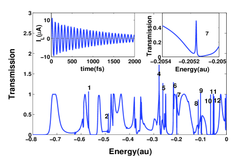
Figure 3: (color online) The transmission coefficient for the CNT-DTB-CNT structure. The insets are $T(E)$ vs energy at peak 7 and its corresponding current.

Let’s examine the contribution of each resonant state to the oscillatory part of the transient current at $v_{L}=0.001au$ (Fig.2a). Among these resonant peaks in Fig.3, the most contribution comes from the peak number 7 with half-width $\Gamma_{7}=2.7\times 10^{-5}au$ which corresponds to a decay time $\tau_{7}=1240fs$ from the expression $\exp(-\Gamma_{7}t)$. In the left inset of Fig.3, we plot the current obtained by integrating ${\rm Tr}[{\cal J}_{\alpha}(\epsilon)]$ over the neighborhood of peak 7 (see right inset of Fig.3). It shows that the decay time is indeed characterized by $\tau_{7}$. Comparing Fig.2 and Fig.3, we see that the contribution from the peak 7 to the total current is about $15\%$ for $t<50fs$ while for $t>50fs$ the contribution is $50\%$. The next dominant contribution is due to the peaks numbered 5, 10, and 12 whose contributions are one order of magnitude smaller. This indicates that one has to include all the resonant peaks for accurate results. Since different resonant peak corresponds to a different half-width $\Gamma$, one can not choose just one $\Gamma$ to characterize the system. We have also calculated the transient current for the structure of $Al-C_{60}-Al$ and our results show that the long time behavior is dominated by two resonant peaks with different $\Gamma$ and shows beat pattern with relaxation time about 800fs.

In summary, we have carried out first principles investigation of time response of molecular devices. We found that the resonant states below Fermi level are crucial for time-dependent quantitative analysis. Our results indicated that the long time behavior of transient current is dominated by resonant states and the individual resonant state gives the damped oscillatory behavior with frequency equal to the bias of pulse and decay rate equal to the life time of the corresponding resonant state. Our results indicated that one has to go beyond the wide-band limit for quantitative calculations of dynamic response of molecular devices.

Acknowledgments: This work was supported by a RGC grant (HKU 704308P) from the government of HKSAR.

References

- (1) : corresponding author.
- (2) S. Kurth et al, Phys. Rev. B 72, 035308 (2005).
- (3) Y. Zhu et al, Phys. Rev. B 71, 075317 (2005).
- (4) X.F. Qian et al, Phys. Rev. B 73, 035408 (2006).
- (5) J. Maciejko et al, Phys. Rev. B 74, 085324 (2006).
- (6) N. Sai et al, Phys. Rev. B 75, 115410 (2007).
- (7) X. Zheng et al, Phys. Rev. B 75, 195127 (2007).
- (8) G. Stefanucci et al, Phys. Rev. B 77, 075339 (2008).
- (9) A.-P. Jauho et al, Phys. Rev. B 50, 5528 (1994).
- (10) E. Runge and E.K.U. Gross, Phys. Rev. Lett. 52, 997 (1984).
- (11) J. Taylor et al, Phys. Rev. B 63 245407 (2001); ibid, 63 121104 (2001).
- (12) M. Brandbyge et al, Phys. Rev. B 65, 165401 (2002).
- (13) N.S. Wingreen et al, Phys. Rev. B 48, 8487 (1993).
- (14) In ab initio calculation, if atomic orbits are chosen, their overlap matrice have to be included in all Green’s functions by replacing with . In this case Eq.(9) has to be divided by a factor .
- (15) In order to use this formalism (Eq.(10)) correctly, one must be careful in the self-energy calculation. In the numerical calculation of self-energy, one usually adds a small imaginary part to the real energy in order to resolve the retarded or advanced self-energies. Unfortunately, this parameter will introduce many spurious poles in the lower half plane with imarginary part of the poles less than . This has no effect on ac current if it is calculated directly. However, if the theorem of residue is used such as Eq.(10) the transient behavior will be dominated by the spurious poles. To eliminate this effect, one has to calculate the self-energy by setting .
- (16) M. Buttiker et al, Phys. Rev. Lett. 70, 4114 (1993).
- (17) B.G. Wang et al, Phys. Rev. Lett. 82, 398 (1999).