A Model of Fermion Masses and Mixings Triggered by Family Problem in Warped Extra Dimensions

Abstract:

We suggest a model which addresses both the fermion mass hierarchy problem and the family problem in two-layer warped extra dimensions. In this model, 3 family fermions in 4 dimensions (4D) generate from 1 family in two-layer warped 6D by two step Kluza-Klein decompositions. The mass hierarchies are produced by the exponential behavior of 4D fermion zero mode profiles. The mixings and masses of fermions are closely related to the family problem. By adjusting parameters in this model, the numerical results can be very close to the experimental data both in the quark sector and in the lepton sector. In the lepton sector, we suppose neutrinos to be Dirac ones. The neutrino masses of sub-$\mathrm{eV}$ scale are obtained, and also CP violation emerges in the lepton sector.

1 Introduction

The Standard Model (SM) is very successful and has been tested by experiments with high precision. However, there still exist puzzles in SM from theoretical perspectives. Two famous ones of them are the family problem and the flavor hierarchy problem. In SM, 3 families of quarks and leptons have similar gauge interactions and it seems that two heavier generations replicate characters of the lightest generation; while the masses of quarks and charged leptons have the obvious hierarchical structure. The hierarchical structure also exists in the Cabibbo-Kobayashi-Maskawa (CKM) mixing matrix. SM accommodates 3 family fermions and their phenomenologies by adjusting the Yukawa couplings. It does not supply an interpretation for the origin of 3 families and the hierarchy structure of flavor parameters.

There have been several different approaches to address these two problems. A natural and popular way is family symmetry. Froggatt and Nielsen [1] suggested a horizontal $U(1)$ symmetry to understand the hierarchical fermion mass structure; while continuous non-Abelian family symmetry, like $SU(3)$, can also lead to very promising results both in the quark sector and in the lepton sector [2]. Recently, triggered by the data from neutrino experiments, discrete non-Abelian family symmetries have attracted many attentions. It is found that the $A_{4}$ family symmetry [3] can produce the famous tri-bimaximal lepton mixing matrix [4], which is a good approximation to the best fit value of the neutrino experimental data [5].

Different from the family symmetry approach, the family and flavor problems are addressed from new approaches in extra dimensional framework. Due to the exponential behavior of fermion profiles in extra dimensions [7, 8], the mass hierarchy of fermions can be produced by parameters of the same order naturally. While family problem also gets new interpretations in extra dimensions. Several groups of authors show that 3 families of SM in 4D can originate from 1 family in 6D [10, 11] by making an appropriate gauge background or choosing a metric of special structure. Although there have been many progresses in these directions, there is still no a well celebrated model to address the family and flavor problems in the community.

In this paper, we focus on the warped extra dimension approach to address the family problem and the flavor problem. In the Randall-Sundrum warped 5D spacetime [12], let fermions to propagate in the bulk. The profiles of fermion zero modes can be of the exponential behavior, which depend on the 5D bulk mass parameters. Due to this character, the fermion mass hierarchy can be reproduced by the 5D bulk mass parameters of the same order. This approach supplies a beautiful geometrical interpretation to the flavor hierarchy problem. In the paper [13], we attempted to understand the origin of the same order 5D bulk mass parameters. The origin of the 5D bulk mass parameters has close relation to the family problem, because one mass parameter can stand for one family. We suggested a two-layer warped 6D spacetime, and begin with 1 family fermion in the 6D bulk. We reduce the spacetime from 6D to 5D at the first step. As a result, the 5D mass parameters emerge as eigenvalues of a 1D Schrödinger-like equation (or Kluza-Klein (KK) modes in 5D). The spacetime metric can be chosen such that only 3 eigenvalues are permitted. So in this setup, 3 families in 5D can originate from 1 family in 6D. When we further reduce the 5D spacetime to the physical 4D at the second step, the zero modes of 3 family fermions in 5D produce 3 family fermions in 4D. By coupling with Higgs field in 4D, these zero modes get masses and produce the 3 family fermions in SM. According to these considerations, we can imagine that both the family problem and the flavor hierarchy problem can be addressed in such an approach. 1 family fermion in 6D produces 3 families in 5D. The 5D mass parameters are of the same order. The same order 5D mass parameters further produce hierarchical structure of fermions in 4D due to the exponential behavior of zero mode profiles. In the following part of this paper, we construct a specific model along the above ideas. We find that the numerical results of this model can be very close to the experimental data by adjusting parameters in this model. The mass hierarchies of quarks and charged leptons are produced. Supposing the neutrinos to be the Dirac ones, the small neutrino masses are obtained. The quark mixing matrix and the lepton mixing matrix are also very close to the realistic CKM matrix and Petrov-Maki-Nakagawa-Sakata (PMNS) matrix respectively.

This paper is organized as follows. In section 2, we simply introduce the model suggested in [13], and develop it to be a more realistic one. We notice several treatments which are different from that in our previous paper [13] in section 2. In section 3, we construct a model along the considerations in the introduction, and adjust the parameters of this model to show that the numerical results can be very close to the experimental data both in the quark sector and in the lepton sector. In section 4, we give some analytical treatments about our model. By these analytical treatments, we show that there are some common concise structures shared by quarks and leptons. We also make some further discussions about this model in section 4. We make summaries in section 5. Several appendices are added for a clear understanding of the paper.

2 Preliminaries for model building

In this section, we introduce some necessary tools for the future model building in section 3. In subsection 2.1, following the discussions in our previous paper [13], we introduce the basic setup to show that how several fermion families in 5D can originate from 1 family in 6D by KK decomposition in two-layer warped extra dimensions. The critical point is how we can get finite KK modes while there are infinite KK modes in the usual KK decomposition. In subsection 2.2, we introduce an example in the popular quantum mechanics textbook to show that finite bound KK modes can be obtained. This simple example helps us to understand the problem more clearly. In subsection 2.3, we make more discussions about the characters of massive KK modes, and analyze an example which will be used in the model building in section 3. In subsection 2.4, we reduce the 5D action to the 4D one, and display the necessary results for model building. In subsection 2.5, we discuss a problem which makes the basic setup in subsection 2.1 to be not realistic. We further suggest a new setup to bypass the problem. This new setup will be used in the model building of section 3, instead of the basic setup in subsection 2.1. In addition, we notice several treatments about the setup which differ from that in our previous paper [13]. We also notice these different treatments in several footnotes. The model building in section 3 largely depends on the discussions in this section.

2.1 Introduction to the basic setup

Following the discussions in [13], we consider a 6D spacetime metric with the special two-layer warped structure,

$$ds^{2}=B(z)^{2}\left[A(y)^{2}\left(\eta_{\mu\nu}dx^{\mu}dx^{\nu}+dy^{2}\right)+dz^{2}\right].$$ (1)

We choose $\eta_{\mu\nu}=\mathrm{diag}(-1,1,1,1)$, and suppose that the two extra dimensions are both intervals.

A massive Dirac fermion in this spacetime has the action

$$S=\int d^{4}xdydz\sqrt{-g}\left\{\frac{i}{2}\left[\bar{\Psi}e_{a}^{M}\Gamma^{a}\nabla_{M}\Psi-\nabla_{M}\bar{\Psi}e_{a}^{M}\Gamma^{a}\Psi\right]-i~{}m\bar{\Psi}\Psi\right\},$$ (2)

where $e_{a}^{M}$ is the sechsbien, and $\nabla_{M}=\partial_{M}+\frac{1}{2}\omega^{ab}_{M}\Gamma_{ab},\Gamma_{ab}=\frac{1}{4}[\Gamma_{a},\Gamma_{b}]$ is the covariant derivative of spinor in curved spacetime. $a$ and $M=0,1,2,3,5,6$ stand for the flat indices and the curved indices in the tetrads respectively. $m$ is a real number to ensure that the action Eq. (2) is hermitian. The gamma matrix representations are as follows,

$$\Gamma^{\mu} = \left(\begin{array}[]{cc}0&\gamma^{\mu}\\ \gamma^{\mu}&0\end{array}\right),~{}\Gamma^{5}=\left(\begin{array}[]{cc}0&\gamma^{5}\\ \gamma^{5}&0\end{array}\right),~{}\Gamma^{6}=\left(\begin{array}[]{cc}\mathbf{1}_{4}&0\\ 0&-\mathbf{1}_{4}\end{array}\right),~{}\Gamma^{7}=\left(\begin{array}[]{cc}0&-i\mathbf{1}_{4}\\ i\mathbf{1}_{4}&0\end{array}\right),$$ (11)

$$\gamma^{0} = \left(\begin{array}[]{cc}0&-\mathbf{1}_{2}\\ \mathbf{1}_{2}&0\end{array}\right),~{}\gamma^{j}=\left(\begin{array}[]{cc}0&\sigma^{j}\\ \sigma^{j}&0\end{array}\right),~{}\gamma^{5}=\left(\begin{array}[]{cc}\mathbf{1}_{2}&0\\ 0&-\mathbf{1}_{2}\end{array}\right),~{}~{}j=1,2,3,$$ (18)

where $\mu=0,1,2,3$ and $\sigma^{j}$ are the Pauli matrices.

As a first step, we reduce the 6D action Eq. (2) to the 5D one by KK decompositions. Rewrite the 6D 8-component spinor with two 4-component spinors and expand these 4-component spinors with 5D fields as follows,

$$\Psi=\left(\begin{array}[]{c}\chi_{1}\\ \chi_{2}\end{array}\right),~{}~{}\chi_{1}(x^{\mu},y,z)=\sum_{n}\widehat{F}_{n}(z)\,\psi_{n}(x^{\mu},y),~{}\chi_{2}(x^{\mu},y,z)=\sum_{n}\widehat{G}_{n}(z)\,\psi_{n}(x^{\mu},y).$$ (21)

Suppose that $\widehat{F}_{n}(z)$ and $\widehat{G}_{n}(z)$ subjugated to the conditions,

$$\left(\frac{d}{dz}+\frac{5}{2}B^{-1}B_{z}\right)\widehat{F}_{n}(z)-mB\widehat{F}_{n}(z)+\lambda_{n}\widehat{G}_{n}(z)=0,$$ (22)

$$\left(\frac{d}{dz}+\frac{5}{2}B^{-1}B_{z}\right)\widehat{G}_{n}(z)+mB\widehat{G}_{n}(z)-\lambda_{n}\widehat{F}_{n}(z)=0,$$ (23)

where $B_{z}=\frac{dB(z)}{dz}$. With the above conditions, the 6D action Eq. (2) is reduced to

$$S = \int d^{4}xdy~{}K_{mn}\left\{\frac{i}{2}A^{4}\left[\bar{\psi}_{m}\gamma^{5}\partial_{5}\psi_{n}-\partial_{5}\bar{\psi}_{m}\gamma^{5}\psi_{n}+\bar{\psi}_{m}\gamma^{\mu}\partial_{\mu}\psi_{n}-\partial_{\mu}\bar{\psi}_{m}\gamma^{\mu}\psi_{n}\right]\right\}$$ (24)

$$- \int d^{4}xdy~{}M_{mn}A^{5}i\bar{\psi}_{m}{\psi}_{n},$$

$$K_{mn} = \int dzB^{5}\left(\widehat{F}_{m}^{\ast}\widehat{F}_{n}+\widehat{G}_{m}^{\ast}\widehat{G}_{n}\right)=\int dz\left({F}_{m}^{\ast}{F}_{n}+{G}_{m}^{\ast}{G}_{n}\right),$$ (25)

$$M_{mn} = \int dzB^{5}\left[\left(\widehat{F}_{m}^{\ast}\widehat{F}_{n}+\widehat{G}_{m}^{\ast}\widehat{G}_{n}\right)\frac{\lambda_{m}^{\ast}+\lambda_{n}}{2}\right]=\int dz\left[\left({F}_{m}^{\ast}{F}_{n}+{G}_{m}^{\ast}{G}_{n}\right)\frac{\lambda_{m}^{\ast}+\lambda_{n}}{2}\right],$$ (26)

where we have defined the transformations

$$\widehat{F}_{n}(z)=B(z)^{-5/2}F_{n}(z),~{}\widehat{G}_{n}(z)=B(z)^{-5/2}G_{n}(z).$$ (27)

The above equations are satisfied for all KK modes, including zero mode and massive modes. By the transformations Eq. (27), equations (22) and (23) can be simplified to

$$\left(\frac{d}{dz}-mB\right)F_{n}(z)+\lambda_{n}G_{n}(z)=0,$$ (28)

$$\left(\frac{d}{dz}+mB\right)G_{n}(z)-\lambda_{n}F_{n}(z)=0.$$ (29)

Our purpose is to obtain the conventional effective 5D action

$$S_{5eff} = \sum_{n}\int d^{4}xdy\left\{\frac{i}{2}A^{4}\left[\bar{\psi}_{n}\gamma^{5}\partial_{5}\psi_{n}-\partial_{5}\bar{\psi}_{n}\gamma^{5}\psi_{n}+\bar{\psi}_{n}\gamma^{\mu}\partial_{\mu}\psi_{n}-\partial_{\mu}\bar{\psi}_{n}\gamma^{\mu}\psi_{n}\right]\right\}$$ (30)

$$- \sum_{n}\int d^{4}xdyA^{5}i\lambda_{n}\bar{\psi}_{n}{\psi}_{n}.$$

We consider two cases:

Case (I): The different KK modes are orthogonal, that is, the normalization conditions

$$K_{mn}=\int dz\left({F}_{m}^{\ast}{F}_{n}+{G}_{m}^{\ast}{G}_{n}\right)=\delta_{mn}$$ (31)

are satisfied. In these conditions, the 6D action Eq. (24) reduce to be the 5D action Eq. (30) naturally.

Case (II): The second case is that the normalization conditions Eq. (31) are not satisfied. In this case, $K$ and $M$ are both matrices. It seems that we can not obtain the conventional effective 5-dimensional action Eq. (30) at first sight. However, if the number of KK modes is finite and the matrix $K$ is positive-definite, we can redefine the fermion fields to obtain an action, which has the same form with that of Eq. (30). The difference is that the eigenvalues $\lambda_{n}$ are modified to different values. The redefinition process can be done in two steps.

Step (1): Decompose the hermitian matrix $K$ as follows,

$$K = V^{\dagger}\Lambda V=H^{\dagger}H,~{}~{}H=\sqrt{\Lambda}V,$$ (32)

$$\Lambda = \mathrm{diag}\left(\Lambda_{1},\Lambda_{2},\cdots,\Lambda_{n}\right),$$

$$\sqrt{\Lambda} = \mathrm{diag}(\sqrt{\Lambda_{1}},\sqrt{\Lambda_{2}},\cdots,\sqrt{\Lambda_{n}}).$$

In the above expressions, $\Lambda_{i}>0,~{}i=1,2,\cdots,n$, as we have supposed that $K$ is positive-definite. Redefine $\psi_{n}$ as

$$\widetilde{\psi}_{m}=H_{mn}\psi_{n},$$ (33)

then in the new basis $\widetilde{\psi}_{n}$, $M$ becomes

$$\widetilde{M}=(H^{-1})^{\dagger}MH^{-1}.$$ (34)

After this step, the kinetic term of Eq. (24) becomes the conventional form as that in Eq. (30);

Step (2): Obviously $\widetilde{M}$ is a hermitian matrix. We can diagonalize this new matrix as

$$\widetilde{M} = U^{\dagger}\Delta U,$$ (35)

$$\Delta = \mathrm{diag}(\widehat{\lambda}_{1},\widehat{\lambda}_{2},\cdots,\widehat{\lambda}_{n}).$$

Redefine also the new basis $\widehat{\psi}_{n}$,

$$\widehat{\psi}_{m}=U_{mn}\widetilde{\psi}_{n}.$$ (36)

We can obtain the action

$$\widehat{S}_{5eff} = \sum_{n}\int d^{4}xdy\left\{\frac{i}{2}A^{4}\left[\bar{\widehat{\psi}}_{n}\gamma^{5}\partial_{5}\widehat{\psi}_{n}-\partial_{5}\bar{\widehat{\psi}}_{n}\gamma^{5}\widehat{\psi}_{n}+\bar{\widehat{\psi}}_{n}\gamma^{\mu}\partial_{\mu}\widehat{\psi}_{n}-\partial_{\mu}\bar{\widehat{\psi}}_{n}\gamma^{\mu}\widehat{\psi}_{n}\right]\right\}$$ (37)

$$- \sum_{n}\int d^{4}xdyA^{5}i\widehat{\lambda}_{n}\bar{\widehat{\psi}}_{n}{\widehat{\psi}}_{n},$$

which has the same form with the action Eq. (30). The total operations on the fermion fields equal to

$$\widehat{\psi} = U\widetilde{\psi}=UH\psi,$$ (38)

$$\mathrm{or}~{}~{}\psi = H^{-1}\widetilde{\psi}=H^{-1}U^{\dagger}\widehat{\psi},$$ (39)

where we have omitted the subscripts.

In the above, beginning with the 6D action Eq. (2), we obtain the 5D action Eq. (30) by KK decompositions. We can interpret this process as follows: the action Eq. (2) stands for 1 fermion family in 6D; while the action Eq. (30) or Eq. (37) can stand for several fermion families in 5D if we can restrict the number of the KK modes to be finite. The masses of these KK modes are determined by the equations (28) and (29). Moreover, it is not necessary to require that these masses have the hierarchical structure. These 5D bulk masses of the same order are enough to produce the hierarchical structure of 4D fermions according to the works in [8]. Therefore, the key point is how we can get finite KK modes. This issue is the theme of the following subsection.

2.2 An example for finite bound KK states from 1D quantum mechanics

Now we analyze the solutions of equations (28) and (29). For a zero mode ($\lambda=0)$, these equations decouple and are easy to be solved. The solutions are given by

$$F_{0}(z)=\frac{1}{\sqrt{lN_{0}}}\mathrm{exp}\left(\int_{z_{0}}^{z}mB(\zeta)d\zeta\right)~{}\mathrm{or}~{}0,G_{0}(z)=\frac{1}{\sqrt{l\widetilde{N}_{0}}}\mathrm{exp}\left(-\int_{z_{0}}^{z}mB(\zeta)d\zeta\right)~{}\mathrm{or}~{}0.~{}$$ (40)

We introduce $l$ of the length dimension in order to make the normalization constants to be dimensionless. For massive modes, we can combine the first order differential equations to obtain second order equations

$$\frac{d^{2}}{dz^{2}}F_{n}(z)+\left[-mB_{z}-m^{2}B^{2}\right]F_{n}(z)+\lambda_{n}^{2}F_{n}(z)=0,$$ (41)

$$\frac{d^{2}}{dz^{2}}G_{n}(z)+\left[mB_{z}-m^{2}B^{2}\right]G_{n}(z)+\lambda_{n}^{2}G_{n}(z)=0.$$ (42)

Rewriting them in another form, we see that they are similar to the 1D Schrödinger equations

$$-\frac{d^{2}}{dz^{2}}F_{n}(z)+V(z)F_{n}(z) = \lambda_{n}^{2}F_{n}(z),$$ (43)

$$-\frac{d^{2}}{dz^{2}}G_{n}(z)+\widetilde{V}(z)G_{n}(z) = \lambda_{n}^{2}G_{n}(z),$$ (44)

with potentials

$$V(z)=mB_{z}+m^{2}B^{2},~{}\widetilde{V}(z)=-mB_{z}+m^{2}B^{2},$$ (45)

where $B_{z}=\frac{dB(z)}{dz}$. In order to obtain the effective 5D action Eq. (30), we should require that the integrands in Eq. (25) and Eq. (26) are finite. These requirements can be satisfied if the KK modes are the bound states of Schrödinger equations (43) and (44). So the problem how we can get finite KK modes transforms to the problem how we can get finite bound states of the 1D Schrödinger equations (43) and (44).

There is a simple example [14] in 1D quantum mechanics which has finite bound states. It is the square potential well of finite depth and width. The potential $V(z)$ is given by

$$V(z)=\begin{cases}0,~{}~{}~{}&\mid z\mid<\frac{a}{2},\\ V,~{}~{}~{}&\mid z\mid>\frac{a}{2},\end{cases}$$ (46)

where $V>0$. The Schrödinger equation is

$$-\frac{{\hbar}^{2}}{2m}\frac{d^{2}}{dz^{2}}u(z)+V(z)u(z)=Eu(z).$$ (47)

The existence of bound states requires that $E<V$. We first consider the case $E>0$. The solutions of Eq. (47) can be classified by parity.

The solution of odd parity is given by

$$u(z)=\begin{cases}-C\exp(\beta z),~{}~{}~{}&z<-\frac{a}{2},\\ B\sin(\alpha z),~{}~{}~{}&\mid z\mid<\frac{a}{2},\\ C\exp(-\beta z),~{}~{}~{}&z>\frac{a}{2},\end{cases}$$ (48)

where $\alpha=\sqrt{\frac{2mE}{{\hbar}^{2}}},~{}\beta=\sqrt{\frac{2m(V-E)}{{\hbar}^{2}}}$. The continuity of $u(z)$ and $\frac{du(z)}{dz}$ at $z=\pm\frac{a}{2}$ requires that

$$-\xi\cot\xi = \eta,$$ (49)

$$\xi^{2}+\eta^{2} = \frac{mV}{2{\hbar}^{2}}a^{2},$$ (50)

where $\xi=\alpha\frac{a}{2},~{}\eta=\beta\frac{a}{2}$.

For the solution of even parity, we obtain

$$u(z)=\begin{cases}C\exp(\beta z),~{}~{}~{}&z<-\frac{a}{2},\\ B\cos(\alpha z),~{}~{}~{}&\mid z\mid<\frac{a}{2},\\ C\exp(-\beta z),~{}~{}~{}&z>\frac{a}{2}.\end{cases}$$ (51)

The continuity conditions require that

$$\xi\tan\xi = \eta,$$ (52)

$$\xi^{2}+\eta^{2} = \frac{mV}{2{\hbar}^{2}}a^{2}.$$ (53)

The eigenvalues are determined by equations (49), (50), (52) and (53). Their number is finite, and the condition that there exist the very $n$ eigenvalues is that

$$\left(\frac{(n-1)\pi}{2}\right)^{2}<\frac{mV}{2\hbar^{2}}a^{2}<\left(\frac{n\pi}{2}\right)^{2}.$$ (54)

From Eq. (54), we know that the number of eigenvalues is restricted by the depth and the width of the square potential well.

In the above, we have discussed the situation $E>0$. However, in the process of KK decomposition, it is not necessary to require that $E>0$. We should also discuss the situation $E<0$. We can obtain solutions of $E<0$ by replacing $\alpha$ and $\xi$ with $i\tilde{\alpha}$ and $i\tilde{\xi}$ in the solutions of $E>0$. We display only the conditions that determine the eigenvalues here. For the odd parity solution, we have

$$-\tilde{\xi}\coth\tilde{\xi} = \eta,$$ (55)

$$-{\tilde{\xi}}^{2}+\eta^{2} = \frac{mV}{2{\hbar}^{2}}a^{2},$$ (56)

and for the even parity solution, we have

$$-\tilde{\xi}\tanh\tilde{\xi} = \eta,$$ (57)

$$-{\tilde{\xi}}^{2}+\eta^{2} = \frac{mV}{2{\hbar}^{2}}a^{2},$$ (58)

where $\tilde{\alpha}=\sqrt{\frac{-2mE}{{\hbar}^{2}}},~{}\tilde{\xi}=\tilde{\alpha}\frac{a}{2}$; while $\beta$ and $\eta$ keep invariant. It is obvious there are no solutions that satisfy the above equations.

In summary, there are finite bound states in the square potential well. This is a simple example to show that it is possible to obtain finite bound states by choosing the potential properly. We are also interested in what kind of metric $B(z)$ can make the square potential well. Replacing $V(z)$ with the square potential well in Eq. (45), we obtain

$$V(z)=mB_{z}+m^{2}B^{2}=\begin{cases}0,~{}~{}~{}&\mid z\mid<\frac{a}{2},\\ V,~{}~{}~{}&\mid z\mid>\frac{a}{2}.\end{cases}$$ (59)

Solving it for $B(z)$, we obtain

$$B(z)=\begin{cases}\frac{1}{mz+C},~{}~{}~{}&\mid z\mid<\frac{a}{2},\\ \frac{\sqrt{V}}{m}\tanh(\sqrt{V}z+\tilde{C}),~{}~{}~{}&\mid z\mid>\frac{a}{2},\end{cases}$$ (60)

where $C$ and $\tilde{C}$ are constants. They can be determined by boundary conditions and continuity conditions. This metric is very similar to that in the papers [15], where the authors opened up the extra dimension at infinity to address the cosmological acceleration problem. For another example for finite bound solutions in different background, see [16].

2.3 General characters of massive modes and an example for model building

In the above subsection, we give an example in 1D quantum mechanics to show that it is possible to obtain finite bound modes. In this subsection, we give another example which also has finite bound modes. This example will be used in the model building of section 3. Before doing that, we analyze some general characters of equations (28) and (29).

The zero mode solution of equations (28) and (29) has been given in Eq. (40). The massive mode solutions are determined by the second order equations (43) and (44). From equations (43) and (44), we see that eigenvalues $\lambda_{n}$ emerge with the form $\lambda_{n}^{2}$; so for $\pm\lambda_{n}$, equations (43) and (44) are both satisfied. In fact, we can infer from equations (28) and (29) that if the pair $(F_{n},G_{n})$ is a solution of equations (28) and (29) corresponding to the eigenvalue $\lambda_{n}$, then another pair $(F_{n},-G_{n})$ is also a solution of equations (28) and (29) corresponding to the eigenvalue $-\lambda_{n}$. Therefore, the massive solutions always emerge in pairs. We denote these pair solutions explicitly as follows,

$$\lambda_{n}\longrightarrow\begin{cases}F_{n}\\ G_{n}\end{cases},~{}~{}~{}~{}~{}-\lambda_{n}\longrightarrow\begin{cases}F_{n}\\ -G_{n}\end{cases}.$$ (61)

Therefore, if these massive modes are discrete, we obtain $(2n+1)$ modes in all, where $n=0,1,2,3,\cdots$, including the zero mode and massive modes. Supposing that there only exist a pair of massive modes, we can write the spectrum of equations (28) and (29) according to above discussions as

$$\mathrm{spectrum~{}of}~{}\lambda\longrightarrow\begin{cases}\lambda_{1}\\ 0\\ -\lambda_{1}\\ \end{cases}.$$ (62)

Now we analyze an example which will be used in the model building of section 3. As in our previous paper [13], we choose the metric $B(z)$ to be

$$B(z)=s\frac{e^{\omega z}+a}{e^{\omega z}+b},~{}~{}s,a,b,\omega>0.$$ (63)

We choose the extent of $z$ to be the semi-infinite interval $[R,~{}\infty)$. This metric is similar to that we obtained in Eq. (60). We implicitly suppose $m>0$ in following discussions, unless we announce it explicitly.

For this metric, the normalizable zero mode solution is given by

$$F_{0}(z)=0,~{}G_{0}(z)=\frac{\sqrt{\omega}}{\sqrt{N_{0}}}\left(\frac{e^{\omega z}}{b}\right)^{-\frac{m}{\omega}s\frac{a}{b}}\left(\frac{e^{\omega z}}{b}+1\right)^{\frac{m}{\omega}s(\frac{a}{b}-1)}.$$ (64)

For massive modes, Eq. (43) can be solved by hypergeometrical functions,

$$F(z) = C_{1}e^{-\mu\omega z}(e^{\omega z}+b)^{\mu-\nu}\mathrm{hypergeom}\left(\rho-\mu+\nu,1-\rho-\mu+\nu;1-2\mu,\frac{e^{\omega z}}{e^{\omega z}+b}\right)$$ (65)

$$+ C_{2}e^{\mu\omega z}(e^{\omega z}+b)^{-\mu-\nu}\mathrm{hypergeom}\left(\rho+\mu+\nu,1-\rho+\mu+\nu;1+2\mu,\frac{e^{\omega z}}{e^{\omega z}+b}\right),~{}~{}$$

where $\rho=\frac{m}{\omega}s(1-\frac{a}{b})$, $\mu=\sqrt{\left(\frac{m}{\omega}s\right)^{2}\left(\frac{a}{b}\right)^{2}-\left(\frac{\lambda}{\omega}\right)^{2}}$, and $\nu=\sqrt{\left(\frac{m}{\omega}s\right)^{2}-\left(\frac{\lambda}{\omega}\right)^{2}}$. $C_{1}$ and $C_{2}$ are constants. We have omitted the subscript $n$ explicitly. We only give the solution for $F(z)$ here. The solution for $G(z)$ can be determined by $F(z)$ through Eq. (28) or by Eq. (44) directly. As discussed in [13], in order to make the solution to be finite when $z\rightarrow\infty$, the hypergeometrical series must be cut off to be a polynomial. This cut off can be completed by four different kinds of choices. We can cut off the series after the coefficient $C_{1}$ by conditions,

$$\rho-\mu+\nu = -n,$$ (66)

$$\mathrm{or}~{}~{}~{}1-\rho-\mu+\nu = -n,$$ (67)

in which $n=0,1,2,3,\cdots$. Otherwise we can cut off the series after the coefficient $C_{2}$ by conditions,

$$\rho+\mu+\nu = -n,$$ (68)

$$\mathrm{or}~{}~{}~{}1-\rho+\mu+\nu = -n.$$ (69)

The four equations (66), (67), (68) and (69) are not necessary to be satisfied at the same time. Anyone of them is enough to cut off the series. So we can obtain four kinds of solutions corresponding to these four different cut off ways generally. The next important task is to analyze whether the number of eigenvalues determined by these equations are finite. We discuss this problem in appendix A. In this subsection, we only display the results.

In this paper, we are interested in the situation $\frac{a}{b}>1$. According to discussions in appendix A, we can have two different ways (66) and (67) to cut off the series. We might obtain two kinds of solutions corresponding to these two cut off ways. While equations (68) and (69) have no solutions, so the corresponding cut off ways do not work. As we analyzed in appendix A, $n$ must be finite in equations (66) and (67). The extents of $n$ are given by equations (374) and (375). For convenience of reading, we copy equations (374) and (375) with new sequence numbers here.

$$\frac{m}{\omega}s\left(\frac{a}{b}-1\right)< n \leq\frac{m}{\omega}s\left[\sqrt{\left(\frac{a}{b}\right)^{2}-1}+\left(\frac{a}{b}-1\right)\right]~{}~{}~{}~{}\mathrm{for~{}~{}(\ref{cut1-a})},$$ (70)

$$-\frac{m}{\omega}s\left(\frac{a}{b}-1\right)< n+1 \leq\frac{m}{\omega}s\left[\sqrt{\left(\frac{a}{b}\right)^{2}-1}-\left(\frac{a}{b}-1\right)\right]~{}~{}~{}~{}\mathrm{for~{}~{}(\ref{cut1-b})}.$$ (71)

From (70) and (71), we know that the number of eigenvalues is determined by a pair of parameters $(\frac{a}{b},~{}\frac{m}{\omega}s)$. We can choose the values of this pair of parameters to make the very two massive modes left. Note that conditions (70) and (71) are not necessary to be satisfied at the same time. They are different restrictions for two kinds of cut off ways respectively.

The values of $(\frac{a}{b},~{}\frac{m}{\omega}s)$ construct a 2D plane. A point set in this 2D plane restricts $n$ to be a specific value. We give a point set of $(\frac{a}{b},~{}\frac{m}{\omega}s)$ determined by following equations

$$\frac{m}{\omega}s\left(\frac{a}{b}-1\right)<1,$$ (72)

$$1<\frac{m}{\omega}s\left[\sqrt{\left(\frac{a}{b}\right)^{2}-1}+\left(\frac{a}{b}-1\right)\right]<2,$$ (73)

$$\frac{m}{\omega}s\left[\sqrt{\left(\frac{a}{b}\right)^{2}-1}-\left(\frac{a}{b}-1\right)\right]<1.$$ (74)

Conditions (72) and (73) imply that only $n=1$ is permitted in Eq. (70); so there is one solution corresponding to this kind of cut off. The condition (74) implies that Eq. (71) is impossible; so there is no solutions corresponding to this kind of cut off. As discussed in the above, the massive modes always emerge in pair. So this parameter set is enough to make a pair massive modes. Together with the zero mode, we obtain the very 3 modes in all. For the future model building, we give solutions for these modes explicitly in appendix B.

The point set determined by equations (72), (73) and (74) forms a specific area in 2D plane. This area can be visualized in Figure. 1.

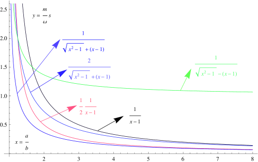
Figure 1: The parameter set for 3 families.

For $\frac{a}{b}>\frac{5}{4}$, this area is given by the area between the curve $y=\frac{1}{\sqrt{x^{2}-1}+(x-1)}$ and the curve $y=\frac{2}{\sqrt{x^{2}-1}+(x-1)}$; while for $\frac{a}{b}<\frac{5}{4}$, this area is given by the area between the curve $y=\frac{1}{\sqrt{x^{2}-1}+(x-1)}$ and the curve $y=\frac{1}{\sqrt{x^{2}-1}-(x-1)}$. However, the points at the curve $y=\frac{1}{2}\frac{1}{x-1}$ must be excluded. As we discussed in appendix A, in this curve, the equation

$$1=2\frac{m}{\omega}s\left(\frac{a}{b}-1\right)$$ (75)

is satisfied. According to Eq. (382), when Eq. (75) is satisfied, $\lambda=0$ for Eq. (66). So in this situation, $n=1$ gives a massless solution but not a massive solution. It is not a new solution and it coincides with the zero mode solution given by Eq. (64). We should exclude the points at this curve in order to ensure that we obtain massive solutions.

2.4 Reducing spacetime from 5D to 4D

We have reduced the spacetime form 6D to 5D in subsection 2.1. In this subsection, we further reduce the spacetime form 5D to 4D. We begin with the effective 5D action (37). Note that masses $\widehat{\lambda}_{n}$ are real irrespective of values of $\lambda_{n}$ in equations (28) and (29), because the induced matrix $\widetilde{M}$ in (34) is hermitian. As in the interval approach of RS model, we choose the extent of $y$ to be a finite interval $[L,~{}L^{\prime}]$.

We make KK decompositions by expanding the 5D field $\widehat{\psi}$ with the 4D chiral fields as

$$\widehat{\psi}=\sum_{j}A(y)^{-2}[f_{L}^{(j)}(y)\psi_{L}^{(j)}+f_{R}^{(j)}(y)\psi_{R}^{(j)}],$$ (76)

where $\psi_{L}=-\gamma^{5}\psi_{L},~{}\psi_{R}=\gamma^{5}\psi_{R}$. In the above expanding, we have omitted the subscript for $\widehat{\psi}$. It is understood that we do the similar operation for each $\widehat{\psi}_{n}$ in the action Eq. (37). The KK modes satisfy following equations

$$\left(\frac{d}{dy}+\hat{\lambda}A\right)f_{L}^{(j)}(y)-\mathbbm{m}^{(j)}f_{R}^{(j)}(y)=0,$$ (77)

$$\left(\frac{d}{dy}-\hat{\lambda}A\right)f_{R}^{(j)}(y)+\mathbbm{m}^{(j)}f_{L}^{(j)}(y)=0,$$ (78)

where $\mathbbm{m}^{(j)}$ are eigenvalues.

In this paper, following a popularly adopted approach in papers [8, 9], we employ the zero mode approximation (ZMA) approach, that is, we solve for the fermion bulk profiles without the brane interaction terms at first and then we treat the brane interaction terms as a perturbation. In this ZMA approach, we can choose two groups of consistent boundary conditions for equations (77) and (78) as follows,

$$\mathrm{Group~{}(I):}~{}~{}\left(\frac{d}{dy}+\hat{\lambda}A\right)f_{L}^{(j)}(y)=0,~{}~{}f_{R}^{(j)}(y)=0,~{}~{}\mathrm{at}~{}~{}y=L~{}~{}\mathrm{and}~{}~{}L^{\prime},$$ (79)

$$\mathrm{Group~{}(II):}~{}~{}\left(\frac{d}{dy}-\hat{\lambda}A\right)f_{R}^{(j)}(y)=0,~{}~{}f_{L}^{(j)}(y)=0,~{}~{}\mathrm{at}~{}~{}y=L~{}~{}\mathrm{and}~{}~{}L^{\prime}.$$ (80)

The boundary conditions (79) save the left-handed zero mode and kill the right-handed one; while the boundary conditions (80) do the opposite.

In the model building in section 3, we will choose the metric factor $A(y)$ to be

$$A(y)=\frac{L}{y},$$ (81)

that is, the RS spacetime. By solving the bulk equations for this metric, we obtain the normalized left-handed zero mode profile and the right-handed one as

$$f_{L}^{(0)}(y) = \frac{1}{\sqrt{L}}\sqrt{\frac{2c-1}{1-\epsilon^{2c-1}}}\left(\frac{y}{L}\right)^{-c},$$ (82)

$$f_{R}^{(0)}(y) = \frac{1}{\sqrt{L}}\sqrt{\frac{-2c-1}{1-\epsilon^{-2c-1}}}\left(\frac{y}{L}\right)^{c},$$ (83)

where $c=\hat{\lambda}L,~{}~{}\epsilon=\frac{L}{L^{\prime}}$, and we suppose that $\epsilon\ll 1$. In this paper, we will also use the canonical normalized zero mode profiles and their values at $y=L^{\prime}$. Their values at $y=L^{\prime}$ are given by

$$\hat{f}_{L}^{(0)} = \sqrt{\frac{2c-1}{1-\epsilon^{2c-1}}}\epsilon^{c-\frac{1}{2}},$$ (84)

$$\hat{f}_{R}^{(0)} = \sqrt{\frac{-2c-1}{1-\epsilon^{-2c-1}}}\epsilon^{-c-\frac{1}{2}},$$ (85)

where $\hat{f}_{L,R}^{(0)}(y)=y^{\frac{1}{2}}f_{L,R}^{(0)}(y)$. For discussions in the next subsection, it is useful to find the asymptotic behavior of these profiles,

$$\hat{f}_{L}^{(0)}\thicksim\begin{cases}\sqrt{1-2c},&\mathrm{for}~{}~{}c<\frac{1}{2},\\ \sqrt{\frac{1}{-\ln{\epsilon}}},~{}&\mathrm{for}~{}~{}c\rightarrow\frac{1}{2},\\ \sqrt{2c-1}~{}\epsilon^{c-\frac{1}{2}},~{}&\mathrm{for}~{}~{}c>\frac{1}{2}.\end{cases}~{}~{}~{}\hat{f}_{R}^{(0)}\thicksim\begin{cases}\sqrt{1+2c},&\mathrm{for}~{}-c<\frac{1}{2},\\ \sqrt{\frac{1}{-\ln{\epsilon}}},~{}&\mathrm{for}~{}-c\rightarrow\frac{1}{2},\\ \sqrt{-1-2c}~{}\epsilon^{-c-\frac{1}{2}},~{}&\mathrm{for}~{}-c>\frac{1}{2}.\end{cases}$$ (86)

We have supposed that $\epsilon\ll 1$ in above expressions.

In the above, we discuss characters of zero modes. In the following we discuss massive modes. For massive modes, equations (77) and (78) can be combined to be the second order equations

$$\frac{d^{2}}{dy^{2}}f_{L}^{(j)}(y)+[\hat{\lambda}A_{y}-\hat{\lambda}^{2}A^{2}]f_{L}^{(j)}(y)+\mathbbm{m}^{(j)2}f_{L}^{(j)}(y)=0,$$ (87)

$$\frac{d^{2}}{dy^{2}}f_{R}^{(j)}(y)+[-\hat{\lambda}A_{y}-\hat{\lambda}^{2}A^{2}]f_{R}^{(j)}(y)+\mathbbm{m}^{(j)2}f_{R}^{(j)}(y)=0,$$ (88)

where $A_{y}=\frac{dA(y)}{dy}$. For the metric (81), equations (87) and (88) can be solved by Bessel functions. Following the standard procedure of analyzing Sturm-Liouville equations, we can obtain from equations (87) and (88) that

$$\left[\mathbbm{m}^{(j)2}-(\mathbbm{m}^{(i)2})^{\ast}\right]\int_{L}^{L^{\prime}}dy\left(f_{L}^{(i)\ast}f_{L}^{(j)}\right) = \left[\left(f_{L}^{(j)}\frac{d}{dy}f_{L}^{(i)\ast}-f_{L}^{(i)\ast}\frac{d}{dy}f_{L}^{(j)}\right)\right]\bigg{|}_{L}^{L^{\prime}},$$ (89)

$$\left[\mathbbm{m}^{(j)2}-(\mathbbm{m}^{(i)2})^{\ast}\right]\int_{L}^{L^{\prime}}dy\left(f_{R}^{(i)\ast}f_{R}^{(j)}\right) = \left[\left(f_{R}^{(j)}\frac{d}{dy}f_{R}^{(i)\ast}-f_{R}^{(i)\ast}\frac{d}{dy}f_{R}^{(j)}\right)\right]\bigg{|}_{L}^{L^{\prime}}.$$ (90)

The above equations are derived from equations (87) and (88) for massive modes, but it also applies for zero modes. The boundary condition (79) ensures that left-handed and right-handed KK modes satisfy orthogonal conditions

$$\int_{L}^{L^{\prime}}dy\left(f_{L}^{(i)\ast}f_{L}^{(j)}\right)=\delta^{ij},~{}~{}\int_{L}^{L^{\prime}}dy\left(f_{R}^{(i)\ast}f_{R}^{(j)}\right)=\delta^{ij}.$$ (91)

While the boundary condition (80) also makes orthogonal conditions (91) satisfied.

2.5 A more realistic setup for model building

According to discussions in subsection 2.3 subsection 2.4, we find a problem which prevents us to construct a realistic model. This problem arises from the following contradiction. On one side, from the asymptotic expressions of the zero mode profiles (86) in subsection 2.4, we know that in order to produce fermion mass hierarchies, the zero mode profiles should be of exponential behavior. According to Eq. (86), because $\epsilon\ll 1$, we need positive parameters $c>\frac{1}{2}$ for left-handed zero mode profile, and negative parameters $-c>\frac{1}{2}$ for right-handed zero mode profile. On the other side, the parameter $c$ comes from the 5D mass $\hat{\lambda}$. We have found in subsection 2.3 that the spectrum of $\hat{\lambda}$ consists of one zero mode and two massive modes $\pm\hat{\lambda}$ in pairs. For left-handed zero modes, $\hat{\lambda}=0$ and $-\hat{\lambda}$ prevent the profiles to have exponential behavior; while for right-handed zero modes, $\hat{\lambda}=0$ and $\hat{\lambda}$ prevent them to have exponential behavior. This contradiction constructs an obstacle to produce the fermion mass hierarchies. In this subsection, we construct a new setup to bypass this problem.

Instead of the action (2), we suggest a new bulk action as follows,

$$S=\int d^{4}xdydz\sqrt{-g}\left\{\frac{i}{2}\left[\bar{\Psi}e_{a}^{N}\Gamma^{a}\nabla_{N}\Psi-\nabla_{N}\bar{\Psi}e_{a}^{N}\Gamma^{a}\Psi\right]-i~{}m\bar{\Psi}\Psi-\mathcal{M}\bar{\Psi}\Gamma^{7}e^{6}_{a}\Gamma^{a}\Psi\right\},$$ (92)

where $\Gamma^{7}$ is defined by Eq. (11). Our metric Ansatz (1) keeps invariant. $\mathcal{M}$ is real to ensure that this new action is hermitian. Comparing it with the action (2), we add a new term. This new term has a strange form, as it breaks the 6D local lorentz invariance obviously. Here we regard this new action as an effective one to bypass the problem discussed above. We will discuss the possible origin of this new action in section 4.

Making the KK decompositions as in subsection 2.1, equations (28) and (29) are modified to be

$$\left(\frac{d}{dz}-mB\right)F_{n}(z)+(\lambda_{n}-\mathcal{M})G_{n}(z)=0,$$ (93)

$$\left(\frac{d}{dz}+mB\right)G_{n}(z)-(\lambda_{n}-\mathcal{M})F_{n}(z)=0.$$ (94)

The induced 5D action is the same with that in equations (24), (25) and (26). The differences are that the KK modes and the eigenvalues $\lambda_{n}$ determined by the new equations (93) and (94) instead of equations (28) and (29). By defining new variables

$$\triangle\lambda_{n}=\lambda_{n}-\mathcal{M},$$ (95)

we obtain

$$\left(\frac{d}{dz}-mB\right)F_{n}(z)+\triangle\lambda_{n}G_{n}(z)=0,$$ (96)

$$\left(\frac{d}{dz}+mB\right)G_{n}(z)-\triangle\lambda_{n}F_{n}(z)=0.$$ (97)

These new equations have the same form with equations (28) and (29). So if we replace $\lambda_{n}$ with $\triangle\lambda_{n}$ in equations (28) and (29), the results that we obtain in subsections 2.2-2.3, appendix A and appendix B apply here. Of course, we should notice that $\lambda_{n}$ in Eq. (95) emerge in actions (24), (25) and (26) but not the new variables $\triangle\lambda_{n}$. We will give more details in section 4. There is a zero mode solution corresponding to $\triangle\lambda=0$, and the massive mode solutions also emerge in pairs. A pair of massive modes for $\triangle\lambda_{n}$ are given by

$$\triangle\lambda_{n}\longrightarrow\begin{cases}F_{n}\\ G_{n}\end{cases},~{}~{}~{}~{}~{}-\triangle\lambda_{n}\longrightarrow\begin{cases}F_{n}\\ -G_{n}\end{cases}.$$ (98)

The spectrum of $\triangle\lambda$ will be the same with that of $\lambda$ given by Eq. (62). While by Eq. (95), the spectrum formula (62) of $\lambda_{n}$ now changes to be

$$\mathrm{spectrum~{}of}~{}\triangle\lambda\longrightarrow\begin{cases}\triangle\lambda_{1}\\ 0\\ -\triangle\lambda_{1}\\ \end{cases}~{}\underrightarrow{\lambda_{n}=\triangle\lambda_{n}+\mathcal{M}}~{}\mathrm{spectrum~{}of}~{}\lambda\longrightarrow\begin{cases}\triangle\lambda_{1}+\mathcal{M}\\ \mathcal{M}\\ -\triangle\lambda_{1}+\mathcal{M}\\ \end{cases}.~{}~{}$$ (99)

By the new spectrum Eq. (99), we can bypass the problem discussed at the onset of this subsection. From equations (96) and (97), we know that $\triangle\lambda_{n}$ depends on the mass parameter $m$ and the metric $B(z)$. So just like we discussed in subsection 2.3, the number and the spectrum of $\triangle\lambda_{n}$ are completely determined by $m$ and parameters in $B(z)$. The number and the spectrum of $\triangle\lambda$ are irrelevant to the new parameter $\mathcal{M}$. We can adjust $\mathcal{M}$ to change the spectrum of the final eigenvalues $\lambda$. If the value of $\mathcal{M}$ is a large positive number, then the spectrum of $\lambda$ can be all positive by Eq. (99), which are expected for left-handed zero modes. We can also make the spectrum of $\lambda$ to be all negative by choosing small negative value of $\mathcal{M}$, which are expected for right-handed zero modes. As we will discuss in subsection 4.1, the new spectrum Eq. (99) for $\lambda$ also applies to $\hat{\lambda}$. The above discussions for $\lambda$ also apply to $\hat{\lambda}$. These features bypass the problem at the beginning of this subsection.

In the model building of section 3, we will adopt this new setup in this subsection. Compared with the setup in subsection 2.1, it is not more difficult to analyze this new setup. We only define the new variable by Eq. (95). All other analysis in subsection 2.2, subsection 2.3, appendix A and appendix B apply here.

3 A model of fermion mass and mixing

In subsection 2.1, we discuss how several families in 5D can generate from 1 family in 6D. In subsection 2.5, we suggest a new setup. By this new setup, we saw that the fermion mass hierarchies in 4D can be produced when we further reduce the spacetime from 5D to 4D. Therefore, we hope that fermion mass hierarchy problem and family problem can be both addressed in such an approach. In such an approach, the mass hierarchy problem will closely relate to the family problem. In this section, we construct a specific model along these discussions. In subsection 3.1, we introduce the model in the 6D bulk spacetime. In order to construct a realistic scenario, we make two assumptions in the model building. In subsection 3.2, in order to obtain a 4D effective theories, we employ two step KK decompositions to reduce the spacetime from 6D to 4D. At the first step, we reduce the spacetime from 6D to 5D, then we further reduce the spacetime from 5D to 4D. After deriving the 4D effective theories, we further give numerical results in subsection 3.3. In subsection 3.3.1, we give numerical results in quark sector. In subsection 3.3.2, supposing neutrinos to be Dirac ones, we apply this model to the lepton sector. In both sectors, the numerical results can be very close to the experimental data. We also give brief comments about the numerical results in subsection 3.3.3.

3.1 Model building

We begin with 6D spacetime with the two-layer warped metric

$$ds^{2}=g_{MN}dx^{M}dx^{N}=B(z)^{2}\left[A(y)^{2}\left(\eta_{\mu\nu}dx^{\mu}dx^{\nu}+dy^{2}\right)+dz^{2}\right].$$ (100)

We also choose the metric factors to be

$$B(z)=s\frac{e^{\omega z}+a}{e^{\omega z}+b},~{}~{}~{}A(y)=\frac{L}{y}.$$ (101)

The parameters in this metric will be designated when we give numerical results in subsection 3.3. As discussed in section 2, we choose the two extra dimensions are both intervals. The extent of $z$ is a semi-infinite interval $[R,~{}\infty]$; while the extent of $y$ is a finite interval $[L,~{}L^{\prime}]$. By these choices, the spacetime is sandwiched by 3 co-dimension 1 4-branes sited at $z=R$, $y=L$ and $y=L^{\prime}$. We also introduce two co-dimension 2 3-branes sited at the brane intersections $(z=R,~{}y=L)$ and $(z=R,~{}y=L^{\prime})$. They can be dubbed UV-brane and IR-brane respectively. We will only designate the field contents on IR-brane sited at $(z=R,~{}y=L^{\prime})$, while the field contents on UV-brane are omitted in the following discussions. The metric on these 3-branes are given by the induced metric

$$g^{\mathrm{hid}}_{\mu\nu}(x)=g_{\mu\nu}(x,R,L),$$ (102)

$$g^{\mathrm{vis}}_{\mu\nu}(x)=g_{\mu\nu}(x,R,L^{\prime}).$$ (103)

We discuss the quark sector at first. We introduce the quark field contents as

$$\mathbb{Q}=\left(\begin{array}[]{c}\mathbb{U}\\ \mathbb{D}\end{array}\right),~{}~{}~{}~{}\mathcal{U},~{}~{}~{}~{}\mathcal{D}.$$ (106)

They transform under the gauge group $\mathrm{SU}(3)_{c}\times\mathrm{SU}(2)_{L}\times\mathrm{U}(1)_{Y}$ as $\mathbb{Q}=(3,2)_{+1/6},~{}\mathcal{U}=(3,1)_{+2/3},~{}\mathcal{D}=(3,1)_{-1/3}$. These fields are 6D fields. Note that there are no family indices for them, that is, we introduce only 1 family in the 6D bulk. Their actions are given by

$$S_{\mathbb{Q}} = \int d^{4}xdydz\sqrt{-g}\bigg{\{}\frac{i}{2}\bigg{[}\bar{\mathbb{Q}}e_{a}^{M}\Gamma^{a}\nabla_{M}\mathbb{Q}-\nabla_{M}\bar{\mathbb{Q}}e_{a}^{M}\Gamma^{a}\mathbb{Q}\bigg{]}-im_{\mathbb{Q}}\bar{\mathbb{Q}}\mathbb{Q}\bigg{\}}$$ (107)

$$- \int d^{4}xdydz\sqrt{-g}\mathcal{M}_{\mathbb{Q}}\bar{\mathbb{Q}}\Gamma^{7}e^{6}_{a}\Gamma^{a}\mathbb{Q},$$

$$S_{\mathcal{U}} = \int d^{4}xdydz\sqrt{-g}\bigg{\{}\frac{i}{2}\bigg{[}\bar{\mathcal{U}}e_{a}^{M}\Gamma^{a}\nabla_{M}\mathcal{U}-\nabla_{M}\bar{\mathcal{U}}e_{a}^{M}\Gamma^{a}\mathcal{U}\bigg{]}-im_{\mathcal{U}}\bar{\mathcal{U}}\mathcal{U}\bigg{\}}$$ (108)

$$- \int d^{4}xdydz\sqrt{-g}\mathcal{M}_{\mathcal{U}}\bar{\mathcal{U}}\Gamma^{7}e^{6}_{a}\Gamma^{a}\mathcal{U},$$

$$S_{\mathcal{D}} = \int d^{4}xdydz\sqrt{-g}\bigg{\{}\frac{i}{2}\bigg{[}\bar{\mathcal{D}}e_{a}^{M}\Gamma^{a}\nabla_{M}\mathcal{D}-\nabla_{M}\bar{\mathcal{D}}e_{a}^{M}\Gamma^{a}\mathcal{D}\bigg{]}-im_{\mathcal{D}}\bar{\mathcal{D}}\mathcal{D}\bigg{\}}$$ (109)

$$- \int d^{4}xdydz\sqrt{-g}\mathcal{M}_{\mathcal{D}}\bar{\mathcal{D}}\Gamma^{7}e^{6}_{a}\Gamma^{a}\mathcal{D}.$$

As in the usual field theory, we introduce the interactions between fermion field and gauge filed by requiring that actions (107), (108) and (109) are invariant under the 6D local gauge transformation

$$\mathbb{Q} \longrightarrow e^{-i[\hat{g}\hat{\theta}_{j}(x,y,z)\frac{\sigma^{j}}{2}+g^{\prime}\tilde{\theta}(x,y,z)]}\mathbb{Q},$$ (110)

$$\mathcal{U} \longrightarrow e^{-ig^{\prime}\tilde{\theta}(x,y,z)}\mathcal{U},~{}~{}\mathcal{D}\longrightarrow e^{-ig^{\prime}\tilde{\theta}(x,y,z)}\mathcal{D},$$

where $\frac{\sigma^{j}}{2}$ are the generators of the gauge group $\mathrm{SU}(2)_{L}$. However, we do not employ this 6D local gauge transformation (110) in this paper. Instead of it, we assume that the fermion actions are only invariant under the 4D local gauge transformation

$$\mathbb{Q} \longrightarrow e^{-i[\hat{g}\hat{\theta}_{j}(x)\frac{\sigma^{j}}{2}+g^{\prime}\tilde{\theta}(x)]}\mathbb{Q},$$ (111)

$$\mathcal{U} \longrightarrow e^{-ig^{\prime}\tilde{\theta}(x)}\mathcal{U},~{}~{}\mathcal{D}\longrightarrow e^{-ig^{\prime}\tilde{\theta}(x)}\mathcal{D}.$$

Here the gauge parameters only depend on the 4D coordinates. Requiring the invariance under transformations Eq. (111), we obtain the interaction terms

$$S_{\mathbb{Q}\mathrm{int}} = -\int d^{4}xdydz\sqrt{-g}\left\{\bar{\mathbb{Q}}e_{a}^{\mu}\Gamma^{a}\bigg{[}\hat{g}W^{j}_{\mu}(x)\frac{\sigma^{j}}{2}+g^{\prime}B_{\mu}(x)\bigg{]}\mathbb{Q}\right\},$$ (112)

$$S_{\mathcal{U}\mathrm{int}} = -\int d^{4}xdydz\sqrt{-g}\left\{\bar{\mathcal{U}}e_{a}^{\mu}\Gamma^{a}[g^{\prime}B_{\mu}(x)]\mathcal{U}\right\},$$ (113)

$$S_{\mathcal{D}\mathrm{int}} = -\int d^{4}xdydz\sqrt{-g}\left\{\bar{\mathcal{D}}e_{a}^{\mu}\Gamma^{a}[g^{\prime}B_{\mu}(x)]\mathcal{D}\right\},$$ (114)

where $\mu=0,1,2,3$. Because we suppose only the 4D local gauge invariance, the gauge field components $W_{5},~{}W_{6}$ and $B_{5},~{}B_{6}$ relevant to extra dimensions are not necessary to be introduced here. These gauge fields only depend on the 4D coordinates. We designate their actions to be the brane actions on the IR-brane

$$S_{\mathrm{gauge}}=\int d^{4}xdydz\sqrt{-g_{\mathrm{vis}}}\left\{-g_{\mathrm{vis}}^{\mu\alpha}g_{\mathrm{vis}}^{\nu\beta}\bigg{[}\frac{1}{4}\hat{F}^{a}_{\mu\nu}\hat{F}^{a}_{\alpha\beta}+\frac{1}{4}\tilde{F}_{\mu\nu}\tilde{F}_{\alpha\beta}\bigg{]}\delta(y-L^{\prime})\delta(z-R)\right\},$$ (115)

where $g_{\mathrm{vis}}^{\mu\alpha}$ is given by Eq. (103).

Note that interaction terms (112), (113) and (114) are different from conventional brane interaction terms

$$S_{\mathbb{Q}\mathrm{int}} = \int d^{4}xdydz\sqrt{-g_{\mathrm{vis}}}\left\{\bar{\mathcal{U}}e_{\mathrm{vis}}^{a\mu}\Gamma_{a}[g^{\prime}B_{\mu}(x)]\mathcal{U}\delta(y-L^{\prime})\delta(z-R)\right\},$$ (116)

where $e_{\mathrm{vis}}^{a\mu},~{}a,\mu=0,1,2,3$ are the tetrad determined by the IR-brane metric $g_{\mathrm{vis}}^{\mu\alpha}$. Interaction terms (112), (113) and (114) are introduced as above to ensure that we can obtain an unitary mixing matrix in the ZMA approach; while the brane interaction terms like Eq. (116) break the unitarity of mixing matrix remarkably in our present model. Interaction terms (112), (113) and (114) are our important assumptions in this paper. We can also introduce gauge fields in the 5D bulk as in the papers [17]. The unitarity of mixing matrix in the ZMA approach is also kept. However, in this paper, we employ the more simple approach as introduced in the above.

Now we introduce the Yukawa interactions between fermion fields and the Higgs fields. We designate them as

$$S_{\mathcal{D}\mathrm{Yukawa}} = \int d^{4}xdydz\sqrt{-g}\left\{\frac{f_{\mathcal{D}}}{\Lambda}[\bar{\mathbb{Q}}\mathcal{D}+\beta_{\mathcal{D}}\bar{\mathbb{Q}}\Gamma^{7}\mathcal{D}]\Phi(x)\frac{L^{\prime}}{L}\delta(y-L^{\prime})+\mathrm{H.C.}\right\},$$ (117)

$$S_{\mathcal{U}\mathrm{Yukawa}} = \int d^{4}xdydz\sqrt{-g}\left\{\frac{f_{\mathcal{U}}}{\Lambda}[\bar{\mathbb{Q}}\mathcal{U}+\beta_{\mathcal{U}}\bar{\mathbb{Q}}\Gamma^{7}\mathcal{U}]\tilde{\Phi}(x)\frac{L^{\prime}}{L}\delta(y-L^{\prime})+\mathrm{H.C.}\right\},$$ (118)

$$\Phi(x) = \frac{1}{\sqrt{2}}\left(\begin{array}[]{c}\phi_{1}(x)+i\phi_{2}(x)\\ \phi_{3}(x)+i\phi_{4}(x)\end{array}\right),~{}\tilde{\Phi}(x)=i\tau^{2}\Phi^{\ast}(x)=\frac{1}{\sqrt{2}}\left(\begin{array}[]{c}\phi_{3}(x)-i\phi_{4}(x)\\ -\phi_{1}(x)+i\phi_{2}(x)\end{array}\right),~{}$$ (123)

where $\Phi(x)$ is a doublet of $\mathrm{SU}(2)_{L}$. $\Lambda$ is a constant with mass dimension. The factor $\frac{L^{\prime}}{L}$ emerges because our metric Ansatz Eq. (100) has the conformal form. If we employ the Gauss normal coordinates for the sub 5D metric, the factor $\frac{L^{\prime}}{L}$ is superfluous. The parameters $f_{\mathcal{U}}$ and $f_{\mathcal{D}}$ are real numbers and dimensionless; while $\beta_{\mathcal{U}}$ and $\beta_{\mathcal{D}}$ can be complex numbers generally. We also introduce the terms after $\beta_{\mathcal{U}}$ and $\beta_{\mathcal{D}}$, which break the parity symmetry of the action. As we will discuss in following subsections, these terms are the origin of CP violation. If we drop these terms, the effective 4D actions will be CP invariant measured by the Jarlskog invariant measure.

Note that the Yukawa interactions are different from the conventional brane Yukawa interactions

$$S_{\mathcal{D}\mathrm{Brane}} = \int d^{4}xdydz\sqrt{-g_{\mathrm{vis}}}\left\{\frac{f_{\mathcal{D}}}{\Lambda}[\bar{\mathbb{Q}}\mathcal{D}+\beta_{\mathcal{D}}\bar{\mathbb{Q}}\Gamma^{7}\mathcal{D}]\Phi(x)\frac{L^{\prime}}{L}\delta(y-L^{\prime})\delta(z-R)\right\}$$ (124)

$$+ \mathrm{H.C.},$$

$$S_{\mathcal{U}\mathrm{Brane}} = \int d^{4}xdydz\sqrt{-g_{\mathrm{vis}}}\left\{\frac{f_{\mathcal{U}}}{\Lambda}[\bar{\mathbb{Q}}\mathcal{U}+\beta_{\mathcal{U}}\bar{\mathbb{Q}}\Gamma^{7}\mathcal{U}]\tilde{\Phi}(x)\frac{L^{\prime}}{L}\delta(y-L^{\prime})\delta(z-R)\right\}$$ (125)

$$+ \mathrm{H.C.}.$$

We adopt interactions (117) and (118) instead of the brane interactions (124) and (125). The reasons are as follows. By the numerical method in section 3.3, we found that interactions (124) and (125) lead to a massless fermion in the ZMA approach in the 4D effective theories. While interactions (117) and (118) can lead to a small but non-zero mass fermion. So we regard interactions (117) and (118) as more plausible choices.

The Higgs field is confined on the 3-brane. Its action is given by the brane action

$$S_{\mathrm{Higgs}}=\int d^{4}x\sqrt{-g_{\mathrm{vis}}}\left\{g_{\mathrm{vis}}^{\mu\nu}D_{\mu}\Phi^{\dagger}D_{\nu}\Phi-\mu_{0}(\Phi^{\dagger}\Phi-v_{0}^{2})^{2}\right\},$$ (126)

where $D_{\mu}=\partial_{\mu}+i\hat{g}W^{j}_{\mu}(x)\frac{\sigma^{j}}{2}+ig^{\prime}B_{\mu}(x)$ is the gauge covariant derivative.

Now we have completed the model building in the 6D bulk. From the above, we know that the gauge field and Higgs field contents are the same with that in SM. The gauge-fixing terms and the ghost fields can be introduced as in SM. We omit them in this paper.

3.2 4D effective theories from the 6D bulk model

We constructed the 6D bulk model in the last subsection. In this subsection, we plan to derive 4D effective theories from the 6D bulk model in subsection 3.1 by KK decompositions. In that 6D bulk model, the gauge fields and the Higgs fields are confined on the brane; while the fermion fields propagate in the bulk. So we only need to reduce the fermion fields from 6D to 4D. The process of reducing fermion fields and relative problems have been discussed in details in section 2. In this subsection, we derive 4D effective theories following discussions in section 2. In subsection 3.2.1, we give general results when we reduce the fermion actions from 6D to 5D by KK decompositions. In subsection 3.2.2, we discuss the special metric Eq. (101). In this example, as we analyzed in subsection 2.3, we can obtain 3 families fermions in 5D by adjusting parameters in the metric. In subsection 3.2.3, we further reduce the actions from 5D to 4D. By this step, we can obtain zero modes in 4D. These zero modes produce the 3 family fermions in SM by coupling with the Higgs fields on the brane.

3.2.1 General discussions about KK decompositions from 6D to 5D

In this subsection, we follow discussions in subsection 2.1. According to Eq. (21), we expand the 6D fields $\mathbb{U}$, $\mathbb{D}$, $\mathcal{U}$ and $\mathcal{D}$ with 5D fields as

$$\mathbb{U} = \left(\begin{array}[]{c}\chi_{\mathbb{U}}^{1}\\ \chi_{\mathbb{U}}^{2}\end{array}\right),\chi_{\mathbb{U}}^{1}(x^{\mu},y,z)=\sum_{n}\widehat{F}^{\mathbb{Q}}_{n}(z)U_{n}(x^{\mu},y),\chi_{\mathbb{U}}^{2}(x^{\mu},y,z)=\sum_{n}\widehat{G}^{\mathbb{Q}}_{n}(z)U_{n}(x^{\mu},y),$$ (129)

$$\mathbb{D} = \left(\begin{array}[]{c}\chi_{\mathbb{D}}^{1}\\ \chi_{\mathbb{D}}^{2}\end{array}\right),\chi_{\mathbb{D}}^{1}(x^{\mu},y,z)=\sum_{n}\widehat{F}^{\mathbb{Q}}_{n}(z)D_{n}(x^{\mu},y),\chi_{\mathbb{D}}^{2}(x^{\mu},y,z)=\sum_{n}\widehat{G}^{\mathbb{Q}}_{n}(z)D_{n}(x^{\mu},y),$$ (132)

$$\mathcal{U} = \left(\begin{array}[]{c}\chi_{\mathcal{U}}^{1}\\ \chi_{\mathcal{U}}^{2}\end{array}\right),\chi_{\mathcal{U}}^{1}(x^{\mu},y,z)=\sum_{n}\widehat{F}^{\mathcal{U}}_{n}(z)\mathscr{U}_{n}(x^{\mu},y),\chi_{\mathcal{U}}^{2}(x^{\mu},y,z)=\sum_{n}\widehat{G}^{\mathcal{U}}_{n}(z)\mathscr{U}_{n}(x^{\mu},y),$$ (135)

$$\mathcal{D} = \left(\begin{array}[]{c}\chi_{\mathcal{D}}^{1}\\ \chi_{\mathcal{D}}^{2}\end{array}\right),\chi_{\mathcal{D}}^{1}(x^{\mu},y,z)=\sum_{n}\widehat{F}^{\mathcal{D}}_{n}(z)\mathscr{D}_{n}(x^{\mu},y),\chi_{\mathcal{D}}^{2}(x^{\mu},y,z)=\sum_{n}\widehat{G}^{\mathcal{D}}_{n}(z)\mathscr{D}_{n}(x^{\mu},y).~{}~{}$$ (138)

Note that we expand $\mathbb{U}$ and $\mathbb{D}$ with the same functions $\widehat{F}^{\mathbb{Q}}_{n}(z)$ and $\widehat{G}^{\mathbb{Q}}_{n}(z)$. Because they are in the same doublet $\mathbb{Q}$ of $\mathrm{SU}(2)_{L}$, they have the same bulk mass parameters by Eq. (107). So they have the same expanding functions. These expanding modes are determined by equations

$$\left(\frac{d}{dz}-m_{\Psi}B\right)F^{\Psi}_{n}(z)+(\lambda^{\Psi}_{n}-\mathcal{M}_{\Psi})G^{\Psi}_{n}(z)=0,$$ (139)

$$\left(\frac{d}{dz}+m_{\Psi}B\right)G^{\Psi}_{n}(z)-(\lambda^{\Psi}_{n}-\mathcal{M}_{\Psi})F^{\Psi}_{n}(z)=0,$$ (140)

where $\Psi$ can stand for $\mathbb{Q}$, $\mathcal{U}$ or $\mathcal{D}$, and we have employed the definitions

$$\widehat{F}^{\Psi}_{n}(z)=B(z)^{-5/2}F^{\Psi}_{n}(z),~{}\widehat{G}^{\Psi}_{n}(z)=B(z)^{-5/2}G^{\Psi}_{n}(z).$$ (141)

By these expanding, the 6D action (107) for $\mathbb{Q}$ is reduced to be

$$S_{\mathbb{Q}} = \int d^{4}xdy~{}K^{\mathbb{Q}}_{mn}\left\{\frac{i}{2}A^{4}\left[\bar{Q}_{m}\gamma^{5}\partial_{5}Q_{n}-\partial_{5}\bar{Q}_{m}\gamma^{5}Q_{n}+\bar{Q}_{m}\gamma^{\mu}\partial_{\mu}Q_{n}-\partial_{\mu}\bar{Q}_{m}\gamma^{\mu}Q_{n}\right]\right\}$$ (144)

$$- \int d^{4}xdy~{}M^{\mathbb{Q}}_{mn}A^{5}i\bar{Q}_{m}{Q}_{n},~{}~{}~{}{Q}_{n}=\left(\begin{array}[]{c}{U}_{n}\\ {D}_{n}\end{array}\right),$$

$$K^{\mathbb{Q}}_{mn} = \int dz\left({F}^{\mathbb{Q}\ast}_{m}{F}^{\mathbb{Q}}_{n}+{G}^{\mathbb{Q}\ast}_{m}{G}^{\mathbb{Q}}_{n}\right),~{}~{}M^{\mathbb{Q}}_{mn}=\int dz\left[\left({F}_{m}^{\mathbb{Q}\ast}{F}^{\mathbb{Q}}_{n}+{G}_{m}^{\mathbb{Q}\ast}{G}^{\mathbb{Q}}_{n}\right)\frac{\lambda_{m}^{\mathbb{Q}\ast}+\lambda^{\mathbb{Q}}_{n}}{2}\right],$$ (145)

where we have combined $U_{n}$ and $D_{n}$ into a doublet $Q_{n}$, because they have the same expanding functions. The action (108) for $\mathcal{U}$ is reduced to be

$$S_{\mathcal{U}} = \int d^{4}xdy~{}K^{\mathcal{U}}_{mn}\left\{\frac{i}{2}A^{4}\left[\bar{\mathscr{U}}_{m}\gamma^{5}\partial_{5}\mathscr{U}_{n}-\partial_{5}\bar{\mathscr{U}}_{m}\gamma^{5}\mathscr{U}_{n}+\bar{\mathscr{U}}_{m}\gamma^{\mu}\partial_{\mu}\mathscr{U}_{n}-\partial_{\mu}\bar{\mathscr{U}}_{m}\gamma^{\mu}\mathscr{U}_{n}\right]\right\}$$ (146)

$$- \int d^{4}xdy~{}M^{\mathcal{U}}_{mn}A^{5}i\bar{\mathscr{U}}_{m}{\mathscr{U}}_{n},$$

$$K^{\mathcal{U}}_{mn} = \int dz\left({F}^{\mathcal{U}\ast}_{m}{F}^{\mathcal{U}}_{n}+{G}^{\mathcal{U}\ast}_{m}{G}^{\mathcal{U}}_{n}\right),~{}~{}M^{\mathcal{U}}_{mn}=\int dz\left[\left({F}_{m}^{\mathcal{U}\ast}{F}^{\mathcal{U}}_{n}+{G}_{m}^{\mathcal{U}\ast}{G}^{\mathcal{U}}_{n}\right)\frac{\lambda_{m}^{\mathcal{U}\ast}+\lambda^{\mathcal{U}}_{n}}{2}\right].$$ (147)

The action (109) for $\mathcal{D}$ is reduced to be

$$S_{\mathcal{D}} = \int d^{4}xdy~{}K^{\mathcal{D}}_{mn}\left\{\frac{i}{2}A^{4}\left[\bar{\mathscr{D}}_{m}\gamma^{5}\partial_{5}\mathscr{D}_{n}-\partial_{5}\bar{\mathscr{D}}_{m}\gamma^{5}\mathscr{D}_{n}+\bar{\mathscr{D}}_{m}\gamma^{\mu}\partial_{\mu}\mathscr{D}_{n}-\partial_{\mu}\bar{\mathscr{D}}_{m}\gamma^{\mu}\mathscr{D}_{n}\right]\right\}$$ (148)

$$- \int d^{4}xdy~{}M^{\mathcal{D}}_{mn}A^{5}i\bar{\mathscr{D}}_{m}{\mathscr{D}}_{n},$$

$$K^{\mathcal{D}}_{mn} = \int dz\left({F}^{\mathcal{D}\ast}_{m}{F}^{\mathcal{D}}_{n}+{G}^{\mathcal{D}\ast}_{m}{G}^{\mathcal{D}}_{n}\right),~{}~{}M^{\mathcal{D}}_{mn}=\int dz\left[\left({F}_{m}^{\mathcal{D}\ast}{F}^{\mathcal{D}}_{n}+{G}_{m}^{\mathcal{D}\ast}{G}^{\mathcal{D}}_{n}\right)\frac{\lambda_{m}^{\mathcal{D}\ast}+\lambda^{\mathcal{D}}_{n}}{2}\right].$$ (149)

Now we consider the interaction sectors under the KK decompositions. For the gauge interaction sector (112), (113) and (114), by the expanding in equations (129)-(138), we obtain

$$S_{\mathbb{Q}\mathrm{int}} = -\int d^{4}xdyA(y)^{4}K^{\mathbb{Q}}_{mn}\left\{\bar{Q}_{m}\gamma^{\mu}\bigg{[}\hat{g}W^{j}_{\mu}(x)\frac{\sigma^{j}}{2}+g^{\prime}B_{\mu}(x)\bigg{]}Q_{n}\right\},$$ (150)

$$S_{\mathcal{U}\mathrm{int}} = -\int d^{4}xdyA(y)^{4}K^{\mathcal{U}}_{mn}\left\{\bar{\mathscr{U}}_{m}\gamma^{\mu}[g^{\prime}B_{\mu}(x)]\mathscr{U}_{n}\right\},$$ (151)

$$S_{\mathcal{D}\mathrm{int}} = -\int d^{4}xdyA(y)^{4}K^{\mathcal{D}}_{mn}\left\{\bar{\mathscr{D}}_{m}\gamma^{\mu}[g^{\prime}B_{\mu}(x)]\mathscr{D}_{n}\right\},$$ (152)

where matrices $K^{\mathbb{Q}}$, $K^{\mathcal{U}}$ and $K^{\mathcal{D}}$ have been defined by equations (145), (147) and (149) respectively. For the the Yukawa interaction sector (117) and (118), after the KK decompositions, we obtain

$$S_{\mathcal{D}\mathrm{Yukawa}} = \int d^{4}xdyA(y)^{5}\left\{\frac{f_{\mathcal{D}}}{\Lambda}[{\mathcal{Y}}^{D}_{mn}+i\beta_{\mathcal{D}}Y^{D}_{mn}]\bar{Q}_{m}\mathscr{D}_{n}\Phi(x)\frac{L^{\prime}}{L}\delta(y-L^{\prime})+\mathrm{H.C.}\right\},$$ (153)

$${\mathcal{Y}}^{D}_{mn} = \int dzB(z)\left({F}^{\mathbb{Q}\ast}_{m}{G}^{\mathcal{D}}_{n}+{G}^{\mathbb{Q}\ast}_{m}{F}^{\mathcal{D}}_{n}\right),Y^{D}_{mn}=\int dzB(z)\left({F}^{\mathbb{Q}\ast}_{m}{F}^{\mathcal{D}}_{n}-{G}^{\mathbb{Q}\ast}_{m}{G}^{\mathcal{D}}_{n}\right),$$ (154)

$$S_{\mathcal{U}\mathrm{Yukawa}} = \int d^{4}xdyA(y)^{5}\left\{\frac{f_{\mathcal{U}}}{\Lambda}[{\mathcal{Y}}^{U}_{mn}+i\beta_{\mathcal{U}}Y^{U}_{mn}]\bar{Q}_{m}\mathscr{U}_{n}\tilde{\Phi}(x)\frac{L^{\prime}}{L}\delta(y-L^{\prime})+\mathrm{H.C.}\right\},$$ (155)

$${\mathcal{Y}}^{U}_{mn} = \int dzB(z)\left({F}^{\mathbb{Q}\ast}_{m}{G}^{\mathcal{U}}_{n}+{G}^{\mathbb{Q}\ast}_{m}{F}^{\mathcal{U}}_{n}\right),Y^{U}_{mn}=\int dzB(z)\left({F}^{\mathbb{Q}\ast}_{m}{F}^{\mathcal{U}}_{n}-{G}^{\mathbb{Q}\ast}_{m}{G}^{\mathcal{U}}_{n}\right).~{}~{}$$ (156)

In the above, we obtain 5D effective actions by KK decompositions. We have not consider the concrete form of the metric $B(z)$. In next subsection, we choose the metric $B(z)$ to be that in Eq. (101), and discuss the further simplifications of the above 5D effective actions.

3.2.2 Deriving 5D effective theories for finite families

In subsection 3.2.1, we obtain the 5D effective actions for a general metric $B(z)$. In this subsection, we plan to obtain 5D effective actions which include only finite KK modes. As we analyzed in section 2, one can obtain finite KK modes by choose a special form of the metric $B(z)$. In this paper, we choose the metric $B(z)$ to be that in Eq. (101). This metric has been analyzed in subsection 2.3 and in our previous paper [13]. The results are that we can cut off the hypergeometrical series by requiring that it is finite when $z\rightarrow\infty$. This requirement determines the solutions uniquely up to the normalization constants. So we do not have freedom to imposing boundary conditions at the other boundary $z=R$. This implies that the normalization conditions Eq. (31) are not be satisfied, and we must change to the case (II) in subsection 2.1. In this case, we should redefine the fermion fields to obtain the conventional 5D effective actions like that in Eq. (37). As in subsection 2.1, we can make these redefinitions in two steps.

Step (I): At this step, we analyze the kinetic terms of fermion actions. As the step (1) in subsection 2.1, we make the Cholesky decompositions for matrices $K$ in the kinetic terms as follows,

$$K^{\mathbb{Q}}=H^{\mathbb{Q}\dagger}H^{\mathbb{Q}},~{}~{}K^{\mathcal{U}}=H^{\mathcal{U}\dagger}H^{\mathcal{U}},~{}~{}K^{\mathcal{D}}=H^{\mathcal{D}\dagger}H^{\mathcal{D}}.$$ (157)

One can make Cholesky decomposition for matrix $K$ only when $K$ is a positive-definite hermitian matrix. In the numerical examples in subsection 3.3.1 and subsection 3.3.2, this condition is satisfied. Redefine the fermion fields as

$$\widetilde{Q}_{m}=H^{\mathbb{Q}}_{mn}Q_{n},~{}~{}\widetilde{\mathscr{U}}_{m}=H^{\mathcal{U}}_{mn}\mathscr{U}_{n},~{}~{}\widetilde{\mathscr{D}}_{m}=H^{\mathcal{D}}_{mn}\mathscr{D}_{n}.$$ (158)

In these new basis, the kinetic terms become the conventional ones similar to that of Eq. (37); while the mass terms are modified to be

$$\widetilde{M}^{\mathbb{Q}}=(H^{\mathbb{Q}-1})^{\dagger}MH^{\mathbb{Q}-1},~{}~{}\widetilde{M}^{\mathcal{U}}=(H^{\mathcal{U}-1})^{\dagger}MH^{\mathcal{U}-1},~{}~{}\widetilde{M}^{\mathcal{D}}=(H^{\mathcal{D}-1})^{\dagger}MH^{\mathcal{D}-1}.$$ (159)

The fermions actions in the new basis are given by

$$S_{\mathcal{Q}} = \int d^{4}xdy~{}\left\{\frac{i}{2}A^{4}\delta_{mn}\left[\bar{\widetilde{\Psi}}_{m}\gamma^{5}\partial_{5}\widetilde{\Psi}_{n}-\partial_{5}\bar{\widetilde{\Psi}}_{m}\gamma^{5}\widetilde{\Psi}_{n}+\bar{\widetilde{\Psi}}_{m}\gamma^{\mu}\partial_{\mu}\widetilde{\Psi}_{n}-\partial_{\mu}\bar{\widetilde{\Psi}}_{m}\gamma^{\mu}\widetilde{\Psi}_{n}\right]\right\}$$ (160)

$$- \int d^{4}xdy~{}\widetilde{M}^{\mathcal{Q}}_{mn}A^{5}i\bar{\widetilde{\Psi}}_{m}{\widetilde{\Psi}}_{n},$$

where $\mathcal{Q}$ can be $\mathbb{Q}$, $\mathcal{U}$ or $\mathcal{D}$; while the corresponding $\Psi$ can stand for $Q$, $\mathscr{U}$ or $\mathscr{D}$ respectively.

For the gauge interaction sector (150), (151) and (152), by the definitions (158), we obtain

$$S_{\mathbb{Q}\mathrm{int}} = -\int d^{4}xdyA(y)^{4}\left\{\bar{\widetilde{Q}}_{n}\gamma^{\mu}\bigg{[}\hat{g}W^{j}_{\mu}(x)\frac{\sigma^{j}}{2}+g^{\prime}B_{\mu}(x)\bigg{]}\widetilde{Q}_{n}\right\},$$ (161)

$$S_{\mathcal{U}\mathrm{int}} = -\int d^{4}xdyA(y)^{4}\left\{\bar{\widetilde{\mathscr{U}}}_{n}\gamma^{\mu}[g^{\prime}B_{\mu}(x)]\widetilde{\mathscr{U}}_{n}\right\},$$ (162)

$$S_{\mathcal{D}\mathrm{int}} = -\int d^{4}xdyA(y)^{4}\left\{\bar{\widetilde{\mathscr{D}}}_{n}\gamma^{\mu}[g^{\prime}B_{\mu}(x)]\widetilde{\mathscr{D}}_{n}\right\},$$ (163)

where the index $n$ is summed. Like matrices in the kinetic terms, the matrices in this sector become identities by the field redefinitions in Eq. (158).

For the Yukawa interaction sector, after redefinitions (158), we obtain

$$S_{\mathcal{D}\mathrm{Yukawa}} = \int d^{4}xdyA(y)^{5}\left\{\frac{f_{\mathcal{D}}}{\Lambda}[\widetilde{{\mathcal{Y}}}^{D}_{mn}+i\beta_{\mathcal{D}}\widetilde{Y}^{D}_{mn}]\bar{\widetilde{Q}}_{m}\widetilde{\mathscr{D}}_{n}\Phi(x)\frac{L^{\prime}}{L}\delta(y-L^{\prime})+\mathrm{H.C.}\right\},$$ (164)

$$\widetilde{{\mathcal{Y}}}^{D} = (H^{\mathbb{Q}-1})^{\dagger}{\mathcal{Y}}^{D}H^{\mathcal{D}-1},~{}~{}\widetilde{Y}^{D}=(H^{\mathbb{Q}-1})^{\dagger}Y^{D}H^{\mathcal{D}-1},$$ (165)

$$S_{\mathcal{U}\mathrm{Yukawa}} = \int d^{4}xdyA(y)^{5}\left\{\frac{f_{\mathcal{U}}}{\Lambda}[\widetilde{{\mathcal{Y}}}^{U}_{mn}+i\beta_{\mathcal{U}}\widetilde{Y}^{U}_{mn}]\bar{\widetilde{Q}}_{m}\widetilde{\mathscr{U}}_{n}\tilde{\Phi}(x)\frac{L^{\prime}}{L}\delta(y-L^{\prime})+\mathrm{H.C.}\right\},$$ (166)

$$\widetilde{{\mathcal{Y}}}^{U} = (H^{\mathbb{Q}-1})^{\dagger}{\mathcal{Y}}^{U}H^{\mathcal{U}-1},~{}~{}\widetilde{Y}^{U}=(H^{\mathbb{Q}-1})^{\dagger}Y^{U}H^{\mathcal{U}-1}.$$ (167)

The Yukawa interaction matrices are modified by the field redefinitions Eq. (158).

In the above, we have completed the first step. This step is to make the kinetic terms of fermion actions to be the conventional ones. The mass matrices and the interaction sectors are modified accordingly. Especially, the gauge interaction sector becomes the flavor universal one, which is important to ensure the unitarity of the mixing matrix in the ZMA approach.

Step (II): At the second step, we diagonalize the mass marix in the action (160). These matrices are hermitian, as they are defined in Eq. (159). They are diagonalized as

$$\widetilde{M}^{\mathbb{Q}} = U^{\mathbb{Q}\dagger}\Delta_{\mathbb{Q}}U^{\mathbb{Q}},~{}~{}\Delta_{\mathbb{Q}}=\mathrm{diag}(\hat{\lambda}^{\mathbb{Q}}_{1},\hat{\lambda}^{\mathbb{Q}}_{2},\cdots,\hat{\lambda}^{\mathbb{Q}}_{n}),$$ (168)

$$\widetilde{M}^{\mathcal{U}} = U^{\mathcal{U}\dagger}\Delta_{\mathcal{U}}U^{\mathcal{U}},~{}~{}\Delta_{\mathcal{U}}=\mathrm{diag}(\hat{\lambda}^{\mathcal{U}}_{1},\hat{\lambda}^{\mathcal{U}}_{2},\cdots,\hat{\lambda}^{\mathcal{U}}_{n}),$$ (169)

$$\widetilde{M}^{\mathcal{D}} = U^{\mathcal{D}\dagger}\Delta_{\mathcal{D}}U^{\mathcal{D}},~{}~{}\Delta_{\mathcal{D}}=\mathrm{diag}(\hat{\lambda}^{\mathcal{D}}_{1},\hat{\lambda}^{\mathcal{D}}_{2},\cdots,\hat{\lambda}^{\mathcal{D}}_{n}).$$ (170)

Redefining the fields in Eq. (160) as

$$\widehat{Q}_{m}=U^{\mathbb{Q}}_{mn}\widetilde{Q}_{n},~{}~{}\widehat{\mathscr{U}}_{m}=U^{\mathcal{U}}_{mn}\widetilde{\mathscr{U}}_{n},~{}~{}\widehat{\mathscr{D}}_{m}=U^{\mathcal{D}}_{mn}\widetilde{\mathscr{D}}_{n}.$$ (171)

These transformations are unitary. So the kinetic terms keep invariant; while the mass terms become the diagonal ones. By these transformations, the action (160) becomes the conventional one

$$S_{\mathcal{Q}} = \sum_{n}\int d^{4}xdy~{}\left\{\frac{i}{2}A^{4}\left[\bar{\widehat{\Psi}}_{n}\gamma^{5}\partial_{5}\widehat{\Psi}_{n}-\partial_{5}\bar{\widehat{\Psi}}_{n}\gamma^{5}\widehat{\Psi}_{n}+\bar{\widehat{\Psi}}_{n}\gamma^{\mu}\partial_{\mu}\widehat{\Psi}_{n}-\partial_{\mu}\bar{\widehat{\Psi}}_{n}\gamma^{\mu}\widehat{\Psi}_{n}\right]\right\}$$ (172)

$$- \sum_{n}\int d^{4}xdy~{}\hat{\lambda}^{\mathcal{Q}}_{n}A^{5}i\bar{\widehat{\Psi}}_{n}{\widehat{\Psi}}_{n}.$$

For the gauge interaction sector, by the unitary transformations (171), we obtain

$$S_{\mathbb{Q}\mathrm{int}} = -\int d^{4}xdyA(y)^{4}\left\{\bar{\widehat{Q}}_{n}\gamma^{\mu}\bigg{[}\hat{g}W^{j}_{\mu}(x)\frac{\sigma^{j}}{2}+g^{\prime}B_{\mu}(x)\bigg{]}\widehat{Q}_{n}\right\},$$ (173)

$$S_{\mathcal{U}\mathrm{int}} = -\int d^{4}xdyA(y)^{4}\left\{\bar{\widehat{\mathscr{U}}}_{n}\gamma^{\mu}[g^{\prime}B_{\mu}(x)]\widehat{\mathscr{U}}_{n}\right\},$$ (174)

$$S_{\mathcal{D}\mathrm{int}} = -\int d^{4}xdyA(y)^{4}\left\{\bar{\widehat{\mathscr{D}}}_{n}\gamma^{\mu}[g^{\prime}B_{\mu}(x)]\widehat{\mathscr{D}}_{n}\right\}.$$ (175)

Because the transformations in Eq. (171) are unitary. They keep universal for the flavors still.

For the Yukawa interaction sector, after redefinitions Eq. (171), we obtain

$$S_{\mathcal{D}\mathrm{Yukawa}} = \int d^{4}xdyA(y)^{5}\left\{\frac{f_{\mathcal{D}}}{\Lambda}[\widehat{{\mathcal{Y}}}^{D}_{mn}+i\beta_{\mathcal{D}}\widehat{Y}^{D}_{mn}]\bar{\widehat{Q}}_{m}\widehat{\mathscr{D}}_{n}\Phi(x)\frac{L^{\prime}}{L}\delta(y-L^{\prime})+\mathrm{H.C.}\right\},$$ (176)

$$\widehat{{\mathcal{Y}}}^{D} = U^{\mathbb{Q}}(H^{\mathbb{Q}-1})^{\dagger}{\mathcal{Y}}^{D}H^{\mathcal{D}-1}U^{\mathcal{D}\dagger},~{}~{}\widehat{Y}^{D}=U^{\mathbb{Q}}(H^{\mathbb{Q}-1})^{\dagger}Y^{D}H^{\mathcal{D}-1}U^{\mathcal{D}\dagger},$$ (177)

$$S_{\mathcal{U}\mathrm{Yukawa}} = \int d^{4}xdyA(y)^{5}\left\{\frac{f_{\mathcal{U}}}{\Lambda}[\widehat{{\mathcal{Y}}}^{U}_{mn}+i\beta_{\mathcal{U}}\widehat{Y}^{U}_{mn}]\bar{\widehat{Q}}_{m}\widehat{\mathscr{U}}_{n}\tilde{\Phi}(x)\frac{L^{\prime}}{L}\delta(y-L^{\prime})+\mathrm{H.C.}\right\},$$ (178)

$$\widehat{{\mathcal{Y}}}^{U} = U^{\mathbb{Q}}(H^{\mathbb{Q}-1})^{\dagger}{\mathcal{Y}}^{U}H^{\mathcal{U}-1}U^{\mathcal{U}\dagger},~{}~{}\widehat{Y}^{U}=U^{\mathbb{Q}}(H^{\mathbb{Q}-1})^{\dagger}Y^{U}H^{\mathcal{U}-1}U^{\mathcal{U}\dagger}.$$ (179)

The interaction matrices are modified by the unitary transformations (171).

Now we complete the second step. This step makes the fermion mass terms to be diagonal ones. After this second step, we obtain the conventional 5D effective fermion action (172). The interaction sectors are modified by unitary transformations (171) accordingly. The gauge interaction sector are still universal for flavors after this step.

We make some summaries about this subsection. By choosing the parameters in the metric, we can obtain finite KK modes. Because of this requirement, we must consider the normalization conditions case (II) in subsection 2.1. However, through twice redefinitions of fermion fields, we can also obtain the conventional 5D effective fermion actions. Having obtained the 4D effective actions for finite KK modes, we can derive 4D effective actions from these 5D actions in the next subsection.

3.2.3 4D effective theories from 5D effective theories

In this subsection, we further reduce the actions from 5D to 4D by KK decompositions.

We begin with the 5D effective actions obtained in last subsection. As that in subsection 2.4, we expand the 5D fields with the 4D fields as follows

$$\widehat{U}_{n}(x,y) = \sum_{j}A^{-2}(y)\left[f^{Q(j)}_{n,L}(y)u^{(j)}_{n,L}(x)+f^{Q(j)}_{n,R}(y)u^{(j)}_{n,R}(x)\right],$$ (180)

$$\widehat{D}_{n}(x,y) = \sum_{j}A^{-2}(y)\left[f^{Q(j)}_{n,L}(y)d^{(j)}_{n,L}(x)+f^{Q(j)}_{n,R}(y)d^{(j)}_{n,R}(x)\right],$$ (181)

$$\widehat{\mathscr{U}}_{n}(x,y) = \sum_{j}A^{-2}(y)\left[f^{\mathscr{U}(j)}_{n,L}(y)u^{(j)}_{n,L}(x)+f^{\mathscr{U}(j)}_{n,R}(y)u^{(j)}_{n,R}(x)\right],$$ (182)

$$\widehat{\mathscr{D}}_{n}(x,y) = \sum_{j}A^{-2}(y)\left[f^{\mathscr{D}(j)}_{n,L}(y)d^{(j)}_{n,L}(x)+f^{\mathscr{D}(j)}_{n,R}(y)d^{(j)}_{n,R}(x)\right].$$ (183)

We give some interpretations about these expanding here. In the above expanding, the superscript $j$ stands for different KK modes, while the subscript $n$ can be interpreted as the family index. Note that they are not summed. We have expanded $\widehat{U}_{n}(x,y)$ and $\widehat{D}_{n}(x,y)$ with the same functions $f^{Q(j)}_{n,L}(y)$ and $f^{Q(j)}_{n,R}(y)$, because they have the same bulk mass parameters as shown in last subsection. As in subsection 2.4, we require that these expanding functions satisfy equations

$$\left(\frac{d}{dy}+\hat{\lambda}^{\mathcal{Q}}_{n}A\right)f_{n,L}^{\Psi(j)}(y)-\mathbbm{m}_{n}^{\Psi(j)}f_{n,R}^{\Psi(j)}(y)=0,$$ (184)

$$\left(\frac{d}{dy}-\hat{\lambda}^{\mathcal{Q}}_{n}A\right)f_{n,R}^{\Psi(j)}(y)+\mathbbm{m}_{n}^{\Psi(j)}f_{n,L}^{\Psi(j)}(y)=0,$$ (185)

where $\mathcal{Q}$ can be $\mathbb{Q}$, $\mathcal{U}$ or $\mathcal{D}$ as in last subsection; while $\Psi$ stands for $Q$, $\mathscr{U}$ or $\mathscr{D}$ accordingly. Note that $n$ can be regarded as the family index here and is not summed. For functions $f^{Q(j)}_{n,L}(y)$ and $f^{Q(j)}_{n,R}(y)$, we designate the boundary conditions as in Eq. (79)

$$\left(\frac{d}{dy}+\hat{\lambda}^{\mathbb{Q}}_{n}A\right)f_{n,L}^{Q(j)}(y)=0,~{}~{}f_{n,R}^{Q(j)}(y)=0,~{}~{}\mathrm{at}~{}~{}y=L~{}~{}\mathrm{and}~{}~{}L^{\prime}.$$ (186)

These boundary conditions save left-handed zero modes while kill right-handed ones. These left-handed zero modes make the doublet of $\mathrm{SU}(2)_{L}$. For functions $f^{\mathscr{U}(j)}_{n,L(R)}(y)$ and $f^{\mathscr{D}(j)}_{n,L(R)}(y)$, we designate the boundary conditions as in Eq. (80)

$$\left(\frac{d}{dy}-\hat{\lambda}^{\mathcal{U}}_{n}A\right)f_{n,R}^{\mathscr{U}(j)}(y)=0,~{}~{}f_{n,L}^{\mathscr{U}(j)}(y)=0,~{}~{}\mathrm{at}~{}~{}y=L~{}~{}\mathrm{and}~{}~{}L^{\prime},$$ (187)

$$\left(\frac{d}{dy}-\hat{\lambda}^{\mathcal{D}}_{n}A\right)f_{n,R}^{\mathscr{D}(j)}(y)=0,~{}~{}f_{n,L}^{\mathscr{D}(j)}(y)=0,~{}~{}\mathrm{at}~{}~{}y=L~{}~{}\mathrm{and}~{}~{}L^{\prime}.$$ (188)

These boundary conditions save right-handed zero modes while kill left-handed ones. These right-handed zero modes make the singlets of $\mathrm{SU}(2)_{L}$. As we discussed in subsection 2.4, these boundary conditions ensure that the expanding functions satisfy following normalization conditions

$$\int_{L}^{L^{\prime}}dy\left(f_{n,L}^{\Psi(i)\ast}f_{n,L}^{\Psi(j)}\right)=\delta^{ij},~{}~{}\int_{L}^{L^{\prime}}dy\left(f_{n,R}^{\Psi(i)\ast}f_{n,R}^{\Psi(j)}\right)=\delta^{ij},$$ (189)

where $\Psi$ stands for $Q$, $\mathscr{U}$ or $\mathscr{D}$. Note that $n$ is the family index and is not summed.

By the above expanding (180)-(183) and the normalization conditions (189), the fermion action (172) becomes

$$S_{\psi} = \sum_{n,j}\int d^{4}x~{}\left\{\frac{i}{2}\left[\bar{\psi}_{n}^{(j)}\gamma^{\mu}\partial_{\mu}\psi_{n}^{(j)}-\partial_{\mu}\bar{\psi}_{n}^{(j)}\gamma^{\mu}\psi_{n}^{(j)}\right]-i\mathbbm{m}_{n}^{\psi(j)}\bar{\psi}_{n}^{(j)}{\psi}_{n}^{(j)}\right\},$$ (190)

where $\psi$ can be $u$ or $d$. This action includes zero modes and massive modes. The modes $u_{n}^{(0)}$ and $d_{n}^{(0)}$ are massless here. They obtain mass by coupling with Higgs field as in actions (176) and (178).

For the gauge interaction sector, after the above expanding, we obtain

$$S_{\mathbb{Q}\mathrm{int}} = \int d^{4}x\left\{\bar{Q}_{n,L}^{(0)}\gamma^{\mu}\bigg{[}\hat{g}W^{i}_{\mu}(x)\frac{\sigma^{i}}{2}+g^{\prime}B_{\mu}(x)\bigg{]}{Q}_{n,L}^{(0)}\right\}$$ (193)

$$+ \sum_{j}\int d^{4}x\left\{\bar{Q}_{n}^{(j)}\gamma^{\mu}\bigg{[}\hat{g}W^{i}_{\mu}(x)\frac{\sigma^{i}}{2}+g^{\prime}B_{\mu}(x)\bigg{]}{Q}_{n}^{(j)}\right\},~{}{Q}_{n,L}=\left(\begin{array}[]{c}{u}_{n,L}\\ {d}_{n,L}\end{array}\right),$$

$$S_{\mathcal{U}\mathrm{int}} = \int d^{4}x\left\{\bar{u}_{n,R}^{(0)}\gamma^{\mu}[g^{\prime}B_{\mu}(x)]u_{n,R}^{(0)}\right\}+\sum_{j}\int d^{4}x\left\{\bar{u}_{n}^{(j)}\gamma^{\mu}[g^{\prime}B_{\mu}(x)]u_{n}^{(j)}\right\},$$ (194)

$$S_{\mathcal{D}\mathrm{int}} = \int d^{4}x\left\{\bar{d}_{n,R}^{(0)}\gamma^{\mu}[g^{\prime}B_{\mu}(x)]d_{n,R}^{(0)}\right\}+\sum_{j}\int d^{4}x\left\{\bar{d}_{n}^{(j)}\gamma^{\mu}[g^{\prime}B_{\mu}(x)]d_{n}^{(j)}\right\},$$ (195)

where $n$ can be regarded as the family index and is summed. In the above, we have employed the normalization conditions (189). We have omitted three total minus signs in the above equations. We also isolate zero modes from massive modes obviously. The gauge interactions of zero modes are chiral because of the boundary conditions (186), (187) and (188); while the gauge interactions of massive modes are vector-like. We also see that the gauge interactions are universal for zero modes.

For the Yukawa interaction sector, by the above expanding, we obtain

$$S_{\mathcal{D}\mathrm{Yukawa}} = \int d^{4}xdyA\frac{f_{\mathcal{D}}}{\Lambda}[\widehat{{\mathcal{Y}}}^{D}_{mn}+i\beta_{\mathcal{D}}\widehat{Y}^{D}_{mn}]\sum_{i,j}\left\{f_{m,L}^{Q(i)\ast}f_{n,R}^{\mathscr{D}(j)}\bar{Q}_{m,L}^{(i)}d_{n,R}^{(j)}+f_{m,R}^{Q(i)\ast}f_{n,L}^{\mathscr{D}(j)}\bar{Q}_{m,R}^{(i)}d_{n,L}^{(j)}\right\}$$ (196)

$$\times \Phi(x)\frac{L^{\prime}}{L}\delta(y-L^{\prime})+\mathrm{H.C.},$$

$$S_{\mathcal{U}\mathrm{Yukawa}} = \int d^{4}xdyA\frac{f_{\mathcal{U}}}{\Lambda}[\widehat{{\mathcal{Y}}}^{U}_{mn}+i\beta_{\mathcal{U}}\widehat{Y}^{U}_{mn}]\sum_{i,j}\left\{f_{m,L}^{Q(i)\ast}f_{n,R}^{\mathscr{U}(j)}\bar{Q}_{m,L}^{(i)}u_{n,R}^{(j)}+f_{m,R}^{Q(i)\ast}f_{n,L}^{\mathscr{U}(j)}\bar{Q}_{m,R}^{(i)}u_{n,L}^{(j)}\right\}$$ (197)

$$\times \tilde{\Phi}(x)\frac{L^{\prime}}{L}\delta(y-L^{\prime})+\mathrm{H.C.},$$

where $\widehat{{\mathcal{Y}}}^{D(U)}$ and $\widehat{Y}^{D(U)}$ are defined as in equations (177) and (179). Here $m$ and $n$ are the family indices. They are summed implicitly. These interaction terms include zero modes and massive modes.

3.2.4 Mass matrices and mixing matrix

In the last subsection, we have derived the 4D effective actions from the 5D ones in subsection 3.2.2. In this subsection, we derive the mass matrix for 4D zero modes and their mixing matrix. Before doing that, we convert the gauge field action and the Higgs field action to the canonical forms.

For the gauge field, use the metric (103), the action (115) becomes to be

$$S_{gauge}=\int d^{4}x\left\{-{\eta}^{\mu\alpha}{\eta}^{\nu\beta}\bigg{[}\frac{1}{4}\hat{F}^{a}_{\mu\nu}\hat{F}^{a}_{\alpha\beta}+\frac{1}{4}\tilde{F}_{\mu\nu}\tilde{F}_{\alpha\beta}\bigg{]}\right\},$$ (198)

where ${\eta}^{\mu\alpha}=\mathrm{diag}(-1,1,1,1)$ is the 4D Lorentz metric. Note that we do not need to redefine the gauge fields. So the gauge interaction actions (193), (194) and (195) keep invariant and still apply in this subsection.

In order to convert the Higgs field action to the canonical form, we redefine the Higgs field as

$$\varphi(x)=\left(\tilde{s}\frac{L}{L^{\prime}}\right)\Phi(x),~{}~{}\tilde{s}=s\frac{e^{\omega R}+a}{e^{\omega R}+b}.$$ (199)

By this redefinition and the metric (103), the Higgs action (126) changes to

$$S_{\mathrm{Higgs}}=\int d^{4}x\left\{{\eta}^{\mu\nu}D_{\mu}\varphi^{\dagger}D_{\nu}\varphi-\mu_{0}(\varphi^{\dagger}\varphi-v^{2})^{2}\right\},$$ (200)

where $v=\tilde{s}\frac{L}{L^{\prime}}v_{0}$. For $\tilde{s}\frac{L}{L^{\prime}}\ll 1$, it supplies a beautiful geometrical solution for gauge hierarchy problem suggested by Randall and Sundrum in [12]. Because the gauge fields do not need to be redefined, the gauge covariance derivative keeps with the same form as that in (126).

After the redefinition (199) for Higgs filed, the Yukawa interaction terms (196) and (197) change to be

$$S_{\mathcal{D}\mathrm{Yukawa}} = \int d^{4}xdyA\frac{f_{\mathcal{D}}}{\tilde{s}\Lambda}[\widehat{{\mathcal{Y}}}^{D}_{mn}+i\beta_{\mathcal{D}}\widehat{Y}^{D}_{mn}]\sum_{i,j}\left\{f_{m,L}^{Q(i)\ast}f_{n,R}^{\mathscr{D}(j)}\bar{Q}_{m,L}^{(i)}d_{n,R}^{(j)}+f_{m,R}^{Q(i)\ast}f_{n,L}^{\mathscr{D}(j)}\bar{Q}_{m,R}^{(i)}d_{n,L}^{(j)}\right\}$$ (201)

$$\times \varphi(x)\left(\frac{L^{\prime}}{L}\right)^{2}\delta(y-L^{\prime})+\mathrm{H.C.},$$

$$S_{\mathcal{U}\mathrm{Yukawa}} = \int d^{4}xdyA\frac{f_{\mathcal{U}}}{\tilde{s}\Lambda}[\widehat{{\mathcal{Y}}}^{U}_{mn}+i\beta_{\mathcal{U}}\widehat{Y}^{U}_{mn}]\sum_{i,j}\left\{f_{m,L}^{Q(i)\ast}f_{n,R}^{\mathscr{U}(j)}\bar{Q}_{m,L}^{(i)}u_{n,R}^{(j)}+f_{m,R}^{Q(i)\ast}f_{n,L}^{\mathscr{U}(j)}\bar{Q}_{m,R}^{(i)}u_{n,L}^{(j)}\right\}$$ (202)

$$\times \tilde{\varphi}(x)\left(\frac{L^{\prime}}{L}\right)^{2}\delta(y-L^{\prime})+\mathrm{H.C.}.$$

Following the ZMA approach, we isolate the zero mode terms from above expressions as follows,

$$S_{\mathcal{D}\mathrm{Yukawa}} = \int d^{4}xdyA\frac{f_{\mathcal{D}}}{\tilde{s}\Lambda}[\widehat{{\mathcal{Y}}}^{D}_{mn}+i\beta_{\mathcal{D}}\widehat{Y}^{D}_{mn}]\left\{f_{m,L}^{Q(0)\ast}f_{n,R}^{\mathscr{D}(0)}\bar{Q}_{m,L}^{(0)}d_{n,R}^{(0)}\right\}\varphi(x)\left(\frac{L^{\prime}}{L}\right)^{2}\delta(y-L^{\prime})$$ (203)

$$+ \mathrm{H.C.},$$

$$S_{\mathcal{U}\mathrm{Yukawa}} = \int d^{4}xdyA\frac{f_{\mathcal{U}}}{\tilde{s}\Lambda}[\widehat{{\mathcal{Y}}}^{U}_{mn}+i\beta_{\mathcal{U}}\widehat{Y}^{U}_{mn}]\left\{f_{m,L}^{Q(0)\ast}f_{n,R}^{\mathscr{U}(0)}\bar{Q}_{m,L}^{(0)}u_{n,R}^{(0)}\right\}\tilde{\varphi}(x)\left(\frac{L^{\prime}}{L}\right)^{2}\delta(y-L^{\prime})$$ (204)

$$+ \mathrm{H.C.}.$$

As in SM, after that the Higgs filed develops a vacuum expectation value, the electroweak symmetry breaks. These Yukawa interactions produce mass terms for fermions. From the above, we see that the mass terms are related to the fermion zero mode profiles. We have worked out these profiles in subsection 2.4 and give their approximation behavior there. By these profiles, we obtain the mass matrices for quarks as follows

$$M^{d}_{mn} = \frac{vf_{\mathcal{D}}}{\tilde{s}\Lambda L}[\widehat{\mathcal{Y}}^{D}_{mn}+i\beta_{\mathcal{D}}\widehat{Y}^{D}_{mn}]\hat{f}_{m,L}^{Q(0)\ast}\hat{f}_{n,R}^{\mathscr{D}(0)},$$ (205)

$$M^{u}_{mn} = \frac{vf_{\mathcal{U}}}{\tilde{s}\Lambda L}[\widehat{\mathcal{Y}}^{U}_{mn}+i\beta_{\mathcal{U}}\widehat{Y}^{U}_{mn}]\hat{f}_{m,L}^{Q(0)\ast}\hat{f}_{n,R}^{\mathscr{U}(0)},$$ (206)

where the indices $m$ and $n$ are not summed. The term $Y_{mn}f_{m}f_{n}$ stands for the product of three quantities $Y_{mn}$, $f_{m}$ and $f_{n}$. $v$ is the Higgs vacuum expectation value as in Eq. (200). $\hat{f}_{n,L}^{Q(0)}$, $\hat{f}_{n,R}^{\mathscr{U}(0)}$ and $\hat{f}_{n,R}^{\mathscr{D}(0)}$ are the values of the canonical zero mode profiles as we defined in equations (84) and (85) in subsection 2.4. They are given by

$$\hat{f}_{m,L}^{Q(0)} = \sqrt{\frac{2c^{Q}_{m}-1}{1-\epsilon^{2c^{Q}_{m}-1}}}\epsilon^{c^{Q}_{m}-\frac{1}{2}},~{}~{}c^{Q}_{m}={\hat{\lambda}}^{\mathbb{Q}}_{m}L,$$ (207)

$$\hat{f}_{n,R}^{\mathscr{D}(0)} = \sqrt{\frac{-2c^{\mathscr{D}}_{n}-1}{1-\epsilon^{-2c^{\mathscr{D}}_{n}-1}}}\epsilon^{-c^{\mathscr{D}}_{n}-\frac{1}{2}},~{}~{}c^{\mathscr{D}}_{n}={\hat{\lambda}}^{\mathcal{D}}_{n}L,$$ (208)

$$\hat{f}_{n,R}^{\mathscr{U}(0)} = \sqrt{\frac{-2c^{\mathscr{U}}_{n}-1}{1-\epsilon^{-2c^{\mathscr{U}}_{n}-1}}}\epsilon^{-c^{\mathscr{U}}_{n}-\frac{1}{2}},~{}~{}c^{\mathscr{U}}_{n}={\hat{\lambda}}^{\mathcal{U}}_{n}L,$$ (209)

where ${\hat{\lambda}}^{\mathbb{Q}}_{m}$, ${\hat{\lambda}}^{\mathcal{D}}_{n}$ and ${\hat{\lambda}}^{\mathcal{U}}_{n}$ are determined by equations (168), (169) and (170). We can rewrite above equations with the matrix form as

$$M^{d} = \frac{vf_{\mathcal{D}}}{\tilde{s}\Lambda L}P^{Q}_{L}[\widehat{\mathcal{Y}}^{D}+i\beta_{\mathcal{D}}\widehat{Y}^{D}]P^{\mathscr{D}}_{R},$$ (210)

$$P^{Q}_{L} = \mathrm{diag}(\hat{f}_{1,L}^{Q(0)},\cdots,\hat{f}_{m,L}^{Q(0)}),~{}~{}P^{\mathscr{D}}_{R}=\mathrm{diag}(\hat{f}_{1,R}^{\mathscr{D}(0)},\cdots,\hat{f}_{m,R}^{\mathscr{D}(0)}),$$ (211)

$$M^{u} = \frac{vf_{\mathcal{U}}}{\tilde{s}\Lambda L}P^{Q}_{L}[\widehat{\mathcal{Y}}^{U}+i\beta_{\mathcal{U}}\widehat{Y}^{U}]P^{\mathscr{U}}_{R},$$ (212)

$$P^{Q}_{L} = \mathrm{diag}(\hat{f}_{1,L}^{Q(0)},\cdots,\hat{f}_{m,L}^{Q(0)}),~{}~{}P^{\mathscr{U}}_{R}=\mathrm{diag}(\hat{f}_{1,R}^{\mathscr{U}(0)},\cdots,\hat{f}_{m,R}^{\mathscr{U}(0)}).$$ (213)

These mass matrices are general complex matrices, and are not hermitian matrices. We can make the single-value decompositions for them to derive the mass eigenstates as follows

$$M^{d} = V_{dL}^{\dagger}\mathcal{M}_{d}V_{dR},~{}~{}\mathcal{M}_{d}=\mathrm{diag}(m_{d_{1}},m_{d_{2}},\cdots,m_{d_{n}}),$$ (214)

$$M^{u} = V_{uL}^{\dagger}\mathcal{M}_{u}V_{uR},~{}~{}\mathcal{M}_{u}=\mathrm{diag}(m_{u_{1}},m_{u_{2}},\cdots,m_{u_{n}}),$$ (215)

where $m_{d_{i}(u_{i})}>0$ for $i=1,2,\cdots,n$ according to the definition of single-value decomposition.

As we discussed above, the gauge interaction terms keep the same form with that of equations (193), (194) and (195). The zero modes interact with gauge fields just like that in SM. So we can define the mixing matrix for quarks like that in SM as

$$V_{\mathrm{CKM}} = V_{uL}V_{dL}^{\dagger}.$$ (216)

3.3 Numerical results

In subsection 3.1, we construct our model in 6D bulk. In subsection 3.2, we derive 4D effective actions from the 6D ones by two step KK decompositions. In this subsection, we give numerical examples to show that the results of our model can be very close to the experimental data.

From the model in subsection 3.1, we know that there are many parameters in this model. These parameters are not determined by the model. We need to input these parameters by hand to obtain the numerical results. These parameters can be classified to two groups: the parameters in the metric and the parameters closely related to the fermion mass matrices. Before giving the numerical results, we give some discussions about the permissible extent of the parameters.

We discuss the parameters in the metric at first. For the extent of the extra dimension $y$, we let

$$\epsilon=\frac{L}{L^{\prime}}=10^{-16},~{}\frac{1}{L}=10^{19}~{}\mathrm{GeV},~{}\frac{1}{L^{\prime}}=\mathrm{TeV},$$ (217)

which is necessary to interpret the gauge hierarchy as suggested in [12]. From Eq. (199), we know that $v_{0}$ relates to $v$ by the factor $\tilde{s}\frac{L}{L^{\prime}}$. The choice of Eq. (217) implies that $\tilde{s}\approx 1$ in order to interpret the gauge hierarchy. The value of $\epsilon$ coincides with that in the paper [18]. We designate the boundary value of the dimension $z$ by the equation

$$\frac{e^{\omega R}}{b}=40.$$ (218)

We also designate the value of the parameter $\omega$ in the metric $B(z)$ by the equation

$$\omega L=0.15.$$ (219)

$\omega$ can be regarded as the intrinsic sale of the the dimension $z$. Eq. (219) implies that $\omega$ is about 10 percents of the Planck scale. We designate $a$ in the metric $B(z)$ by the equation

$$\frac{a}{b}=6.$$ (220)

The other parameters like $s$ and $b$ are not necessary designated in the numerical examples as they always emerge in combinations with other parameters.

In the above, we have designated the necessary parameters in the metric. We notice that the values of these parameters are not determined by our model. We expect that they can be determined by some underlying theories, which are not discussed by the present paper. We choose them to the above values by hand in this paper, because we find that these values can make the results of our model to be very close to the experimental data.

3.3.1 Numerical results in quark sector

In this subsection, we give numerical results in the quark sector. The parameters in the metric have been given above. To obtain the numerical results, we need to further designate the parameters related to quark mass matrices. At first, we need to designate the parameters $m$ and $\mathcal{M}$ in actions (107), (108) and (109). From the analysis in subsection 2.3, we know that the number of family is determined by the pair $(\frac{a}{b},\frac{m}{\omega}s)$. So the parameter $\frac{m}{\omega}s$ is closely related to the number of family. In subsection 2.3, we have given a parameter set which permits the very 3 families. As we analyzed in subsection 2.5, these conclusions also apply to the new setup in subsection 2.5. This parameter set is given by equations (72), (73) and (74). We have designated the value of $\frac{a}{b}$ by Eq. (220), so the possible extent for $\frac{m}{\omega}s$ is given by

$$\frac{m}{\omega}s\in(\frac{1}{\sqrt{35}+5},~{}\frac{2}{\sqrt{35}+5})~{}~{}\mathrm{and}~{}~{}\frac{m}{\omega}s\neq\frac{1}{10}.$$ (221)

We exclude the point $\frac{m}{\omega}s=\frac{1}{10}$, because when $\frac{m}{\omega}s=\frac{1}{10}$, we obtain a massless solution, which coincides with the zero mode solution as we discussed in subsection 2.3. The parameters $m$ in actions (107), (108) and (109) should take values in the intervals Eq. (221) to ensure that there are the very 3 families in our model. While $\mathcal{M}$ is irrelevant to the family number. Instead it is closely relevant to the values of quark masses, as it can be seen from the following numerical example. For $m$ in the intervals Eq. (221), the explicit expressions for 3 family KK modes can be determined as we discussed in subsection 2.5. According to those discussions, the solutions are very similar to that given in appendix B. The differences are that we should replace $\lambda$ with $\triangle\lambda$ in the expressions in appendix B. By the normalization conditions Eq. (407), these solutions can be determined completely. The values of $m$ and $\mathcal{M}$ for different fields are different generally. We adjust them by hand to fit the experimental data. We give the values for them in Table. 3.3.1. Note that the negative real numbers $m$ also emerge in Table. 3.3.1. The solutions for this case are also discussed in appendix B.

The Yukawa couplings $f$ and $\beta$ in equations (117) and (118) also need to be input by hand. We give their values in Table. 3.3.1. In Table. 3.3.1, we have defined that

$$\tilde{f}_{\mathcal{U}}=\frac{vf_{\mathcal{U}}}{\Lambda L}\frac{e^{\omega R}+b}{e^{\omega R}+a},~{}~{}~{}\tilde{f}_{\mathcal{D}}=\frac{vf_{\mathcal{D}}}{\Lambda L}\frac{e^{\omega R}+b}{e^{\omega R}+a}.$$ (222)

Table. 3.3.1   Parameters in quark sector
Field	$\frac{m}{\omega}s$	$\frac{\mathcal{M}}{\omega}s$
$\mathbb{Q}$	$0.152$	4.25
$\mathcal{U}$	$-0.173$	$-4.0$
$\mathcal{D}$	$-0.093$	$-4.2$
$\tilde{f}_{\mathcal{U}}$=15.5 TeV	$\beta_{\mathcal{U}}=0.55-0.43i$
$\tilde{f}_{\mathcal{D}}$=12.7 TeV	$\beta_{\mathcal{D}}=-1.2-0.5i$

Having designated these parameters, we can obtain the numerical expressions of kinds of quantities in our model, like the matrices $K$ and mass matrices $M$ in the fermion actions (144), (146) and (148), the eigenvalues $\hat{\lambda}_{n}$ in equation (172) after two step redefinitions of fermion fields and so on. In this paper, we omit these intermediate numerical expressions. We only give the final mass matrices in equations (210) and (212). However, some analytical expressions for these intermediate quantities can be found in subsection 4.1.

By the parameter values given above, we obtain the numerical expressions for mass matrices (210) and (212) as follows.

$$M^{u} = \left(\begin{array}[]{ccc}(6.44+0.552i)\cdot 10^{-4}&(0.922+1.49i)\cdot 10^{-2}&-0.123-0.158i\\ (-1.53-3.25i)\cdot 10^{-3}&0.573&-5.44-4.98i\\ (1.29+1.64i)\cdot 10^{-2}&2.23+2.36i&135.58-13.4i\end{array}\right)~{}\mathrm{GeV},$$ (226)

$$M^{d} = \left(\begin{array}[]{ccc}(0.72+2.78i)\cdot 10^{-3}&(1.1-0.58i)\cdot 10^{-2}&(3.9-7.85i)\cdot 10^{-3}\\ (-6.57+1.8i)\cdot 10^{-3}&4.39\cdot 10^{-2}&(-1.36-0.49i)\cdot 10^{-2}\\ 0.155-0.46i&-0.984-0.93i&-1.30+1.19i\end{array}\right)~{}\mathrm{GeV}.~{}~{}$$ (230)

Making the single-value decompositions as in equations (214) and (215), we obtain the quark masses as follows

$$m_{u} = 0.64~{}\mathrm{MeV},~{}~{}m_{c}=584.87~{}\mathrm{MeV},~{}~{}m_{t}=136.48~{}\mathrm{GeV},$$ (231)

$$m_{d} = 2~{}\mathrm{MeV},~{}~{}m_{s}=36.36~{}\mathrm{MeV},~{}~{}m_{b}=2.278~{}\mathrm{GeV}.$$ (232)

They are consistent with the $\overline{\mathrm{MS}}$ quark masses evaluated at $1.5$ $\mathrm{TeV}$ in the paper [18]. By Eq. (216), the mixing matrix and its absolute value are given by

$$V_{\mathrm{CKM}} = \left(\begin{array}[]{ccc}0.974+0.00614i&0.224545-0.0293i&(4.297-0.58i)\cdot 10^{-3}\\ 0.1488-0.1699i&-0.535961+0.811i&0.0553-0.0232i\\ -0.0011-0.0172i&0.01957+0.0542i&-0.249+0.9666i\end{array}\right),$$ (236)

$$\mid V_{\mathrm{CKM}}\mid = \left(\begin{array}[]{ccc}0.974014&0.226448&0.00433647\\ 0.225832&0.972317&0.0599961\\ 0.0172432&0.0576282&0.998189\end{array}\right).$$ (240)

We also obtain the Jarlskog invariant as

$$J=-\mathrm{Im}(V_{ud}V_{cb}V_{ub}^{*}V_{cd}^{*})=3.20416\times 10^{-5}.$$ (241)

They are very close to the experimental data compiled in [19].

3.3.2 Numerical results in lepton sector

In this subsection, we discuss the lepton sector. We suppose that neutrinos are Dirac ones. In this case, the lepton sector is very similar to the quark sector. For neutrinos in other scenarios, see [20].

We introduce the fermion field contents in the 6D bulk as

$$\mathbb{L}=\left(\begin{array}[]{c}\mathbb{N}\\ \mathbb{E}\end{array}\right),~{}~{}~{}~{}\mathcal{N},~{}~{}~{}~{}\mathcal{E}.$$ (244)

They transform under the gauge group $\mathrm{SU}(3)_{c}\times\mathrm{SU}(2)_{L}\times\mathrm{U}(1)_{Y}$ as $\mathbb{L}=(1,2)_{-1},~{}\mathcal{N}=(1,1)_{0},~{}\mathcal{E}=(1,1)_{-2}$. Note that we also introduce only 1 family lepton in the 6D bulk. The actions of these fields are the same with that in equations (107), (108) and (109). The model in subsection 3.1 applies similarly here, other than there is no color interaction for leptons. The process of deriving 4D effective actions from the 6D ones in subsection 3.2 also applies here. While the mixing matrix for leptons is defined by

$$V_{\mathrm{PMNS}} = V_{lL}^{\dagger}V_{\nu L}.$$ (245)

Now we discuss the parameters in the lepton sector. The parameters in the metric given by equations (217), (218), (219) and (220) still apply in the lepton sector. The parameters $m$ of leptons should also in the intervals Eq. (221) to ensure that we can obtain the very 3 families in the lepton sector. Other parameters should also be input by hand like that in the quark sector. We adjust them by hand to fit the experimental data. We give their values in Table. 3.3.2.

Table. 3.3.2   Parameters in lepton sector
Field	$\frac{m}{\omega}s$	$\frac{\mathcal{M}}{\omega}s$
$\mathbb{L}$	$0.16$	$-9.0$
$\mathcal{N}$	$-0.0944$	$-9.75$
$\mathcal{E}$	$-0.147$	$-5.6$
$\tilde{f}_{\mathcal{N}}$=23.89 TeV	$\beta_{\mathcal{N}}=1.5+0.45i$
$\tilde{f}_{\mathcal{E}}$=21.23 TeV	$\beta_{\mathcal{E}}=0.9752$

Having designating these parameters in lepton sector, we can obtain the numerical expressions for kinds of quantities as in the quark sector. In this subsection, we also only give the mass matrices for leptons. They are given by

$$M^{\nu} = \left(\begin{array}[]{ccc}3.204-8.405i&21.18-13.78i&6.37+26.6i\\ 0.6978+0.632i&-6.286&3.53-2.072i\\ -6.48+7.72i&-12.29-13.11i&5.736-26.22i\end{array}\right)\cdot~{}10^{-3}~{}\mathrm{eV},$$ (249)

$$M^{l} = \left(\begin{array}[]{ccc}0.287455+3.48i&-10.01+90.3488i&1501.6+154.77i\\ -0.4266-6.935i&129.213&58.594-952.495i\\ 10.40-1.072i&9.527+85.96i&37.56-454.82i\end{array}\right)~{}\mathrm{MeV}.$$ (253)

Making single-value decompositions for these matrices as in equations (214) and (215), we obtain the lepton masses as follows

$$m_{e} = 0.511~{}\mathrm{MeV},~{}~{}m_{\mu}=105.229~{}\mathrm{MeV},~{}~{}m_{\tau}=1849.15~{}\mathrm{MeV},$$ (254)

$$m_{1} = 0.0019~{}\mathrm{eV},~{}~{}m_{2}=0.013~{}\mathrm{eV},~{}~{}m_{3}=0.05~{}\mathrm{eV}.$$ (255)

The masses of electron and muon are close to their experimental value; while the mass of $\tau$ is moderately large than its experimental value compiled in [19]. The neutrino masses are of normal hierarchy type. They are close to the experimental values in [5]. We can also obtain the mixing matrix defined in Eq. (245) and its absolute value as

$$V_{\mathrm{PMNS}} = \left(\begin{array}[]{ccc}0.6799-0.4592i&0.5163+0.2442i&0.02504+0.003909i\\ -0.4619-0.02652i&0.2922+0.5664i&0.44075+0.43071i\\ 0.2051-0.2659i&-0.5136-0.06183i&0.7715-0.1561i\end{array}\right),$$ (259)

$$\mid V_{\mathrm{PMNS}}\mid = \left(\begin{array}[]{ccc}0.820465&0.571134&0.02534\\ 0.462666&0.637319&0.61625\\ 0.335822&0.517329&0.78714\end{array}\right).$$ (263)

They are in the $3\sigma$ extent of the experimental values in [5].

We have supposed neutrinos to be Dirac ones. So as in the quark sector, we can calculate the Jarlskog invariant for the mixing matrix as

$$J=-\mathrm{Im}(V_{e1}V_{\mu 3}V_{e3}^{*}V_{\mu 1}^{*})=19.193\times 10^{-5}.$$ (264)

It is lager than that in the quark sector. We note that its size is not the inevitable result of our model. When we adjust the parameters, we find that the size of $J$ is very sensitive to the mass $m$ of the field $\mathcal{N}$. By adjusting $\frac{m_{\mathcal{N}}}{\omega}s$, we can still keep the mixing matrix and the neutrino masses to be close to their experimental values, but $J$ can varies remarkably.

3.3.3 Brief comments on the numerical results

We give the numerical results in the last two subsections. We see that there are still many parameters in our model. The parameters $\frac{\mathcal{M}}{\omega}s$ are closely relevant to the absolute size of the fermion masses. The parameter $\frac{\mathcal{M}}{\omega}s$ of the field $\mathcal{N}$ is more lager than that of quarks and charged leptons, because the neutrino masses are remarkably smaller than the masses of quarks and charged leptons. While the parameters $\frac{m}{\omega}s$ are closely relevant to the mass hierarchy structure of quarks and charged leptons. In general, lager absolute value of $\frac{m}{\omega}s$ produces larger mass hierarchy. The parameters $\beta$ are closely relative to the CP violation measure $J$. $\beta=0$ implies that $J$ vanishes. In the above numerical examples, we see that $\beta\neq 0$ in the lepton sector, so CP violation also emerges in the lepton sector. We have not found a group of parameters with $\beta=0$ which can fit the experimental data as the group of parameters in the last subsection.

We also see that the values of $\frac{\mathcal{M}}{\omega}s$ are about 100 times larger than the values of $\frac{m}{\omega}s$, while this little hierarchy is not explained in this paper. In addition, because there are too many parameters in our model, we only adjust them by hand to obtain the numerical results. These numerical results are very close to the experimental values. We have not done further adjustments to make them in the $1\sigma$ extent permitted by experiments. In the last two subsections, we only give rough numerical examples to show that our model can close to the experimental data in high precision. For the quark masses, we take the renormalization effects into consideration, and adjust the parameters to fit the running masses at $1.5$ $\mathrm{TeV}$ compiled in [18]. While for the leptons masses and the mixing matrices, we only adjust parameters by hand to fit the face values compiled in [5, 19], and the renormalization effects are omitted. So the above numerical examples are only rough treatments. The renormalization effects of these quantities should be considered for more detailed comparison with the experimental data.

4 Some analytical treatments about the model and more relevant discussions

In section 3, we introduce our model and give the numerical results. At first sight, this model seems very complicated. However, when we give some analytical treatments about this model, we will see that some quantities in this model have very concise expressions. We can make some qualitative conclusions from these concise expressions. These analytical treatments can help us to understand how our model works more clearly. In subsection 4.2, we make more discussions about several relevant problems.

4.1 Some analytical treatments about the model

For analytical discussions, we take fields $\mathbb{Q}$ and $\mathcal{D}$ for example. The analytical treatments for $\mathcal{U}$ are very similar to that of $\mathbb{Q}$ and $\mathcal{D}$. As we discussed in appendix B, the solutions for KK modes are different for $m$ to be positive or negative. While the eigenvalues $\lambda$ determined by equations (66), (67), (68) and (69) can be real or pure imaginary according to the parameter pair $(\frac{a}{b},~{}\frac{m}{\omega}s)$. The analytical expressions can be classified into four classes: (1) $m>0$, $\lambda$ is real; (2) $m>0$, $\lambda$ is pure imaginary; (3) $m<0$, $\lambda$ is real; (4) $m<0$, $\lambda$ is pure imaginary. For the new setup in subsection 2.5, we should replace $\lambda$ with $\triangle\lambda$ as we analyzed in subsection 2.5. In the numerical examples for quark sector in subsection 3.3.1. The solutions for $\mathbb{Q}$ belong to the class (2); while the solutions for $\mathcal{D}$ belong to the class (3). The solutions for $\mathcal{U}$ belong to the class (4). In the following discussions, we always suppose that the solutions for $\mathbb{Q}$ belong to the class (2) and the solutions for $\mathcal{D}$ belong to the class (3). Other situations can be discussed similarly.

For the analytical treatments, we must discuss the solutions for KK modes at first. The solutions can be determined according to our discussions in subsection 2.5. They have the similar forms and characters to that given in appendix B. By these solutions, we obtain the expressions for the matrices $K$ and $M$ in the fermion actions (144) and (148) as follows

$$K^{\mathbb{Q}} = \left(\begin{array}[]{ccc}1&ia_{\mathbb{Q}}&-ia_{\mathbb{Q}}\\ -ia_{\mathbb{Q}}&1&b_{\mathbb{Q}}\\ ia_{\mathbb{Q}}&b_{\mathbb{Q}}&1\end{array}\right),M^{\mathbb{Q}}=\mathcal{M}_{\mathbb{Q}}K^{\mathbb{Q}}+\left(\begin{array}[]{ccc}0&\tilde{a}_{\mathbb{Q}}&\tilde{a}_{\mathbb{Q}}\\ \tilde{a}_{\mathbb{Q}}&0&-i\tilde{b}_{\mathbb{Q}}\\ \tilde{a}_{\mathbb{Q}}&i\tilde{b}_{\mathbb{Q}}&0\end{array}\right),$$ (271)

$$K^{\mathcal{D}} = \left(\begin{array}[]{ccc}1&a_{\mathcal{D}}&-a_{\mathcal{D}}\\ a_{\mathcal{D}}&1&b_{\mathcal{D}}\\ -a_{\mathcal{D}}&b_{\mathcal{D}}&1\end{array}\right),~{}~{}M^{\mathcal{D}}=\mathcal{M}_{\mathcal{D}}K^{\mathcal{D}}+\left(\begin{array}[]{ccc}0&\tilde{a}_{\mathcal{D}}&\tilde{a}_{\mathcal{D}}\\ \tilde{a}_{\mathcal{D}}&\triangle\lambda^{\mathcal{D}}&0\\ \tilde{a}_{\mathcal{D}}&0&-\triangle\lambda^{\mathcal{D}}\end{array}\right),$$ (278)

where we have used the normalization conditions in Eq. (407). We give the expressions for $a_{\mathbb{Q}}$, $a_{\mathcal{D}}$, $b_{\mathbb{Q}}$ and $b_{\mathcal{D}}$ in equations (408) and (409) in appendix C. They are all real numbers by definitions. Here and in the following, we arrange the column and the row indices for the matrices as $0,1,-1$, which are the indices for KK modes displayed in appendix B. $\triangle\lambda$ are the eigenvalues in equations (96) and (97). They can be calculated according to our discussions in subsection 2.5. We have employed Eq. (95) to rewrite the expressions for mass matrices $M$.

Now we discuss the matrices in interaction sectors. For the gauge interaction sector, from equations (150) and (152), we know that the matrices in this sector are the same with that in the above. The matrices in the Yukawa interaction sector are important for our discussions. We obtain expressions for these matrices in Eq. (154) as follows

$$\mathcal{Y}^{D} = \left(\begin{array}[]{ccr}\mathbbm{s}&\mathbbm{a}&-\mathbbm{a}\\ \mathbbm{b}&\mathbbm{c}&\mathbbm{d}\\ -\mathbbm{b}&\mathbbm{d}&\mathbbm{c}\end{array}\right),~{}~{}~{}Y^{D}=\left(\begin{array}[]{ccr}0&\mathbbm{a}^{\prime}&\mathbbm{a}^{\prime}\\ \mathbbm{b}^{\prime}&\mathbbm{c}^{\prime}&\mathbbm{d}^{\prime}\\ \mathbbm{b}^{\prime}&-\mathbbm{d}^{\prime}&-\mathbbm{c}^{\prime}\end{array}\right).$$ (285)

The elements in these matrices are defined by equations (410) and (411) in appendix C. These elements can be complex numbers generically.

From the analytical expressions above, we see that these matrices all have very concise structures. Following the procedures in subsection 3.2.2, we need two steps to obtain conventional 5D effective actions.

Step (I): Making Cholesky decompositions for the matrices $K$, for the field $\mathbb{Q}$, we obtain

$$K^{\mathbb{Q}} = V^{\mathbb{Q}\dagger}\Lambda^{\mathbb{Q}}V^{\mathbb{Q}}=H^{\mathbb{Q}\dagger}H^{\mathbb{Q}},~{}H^{\mathbb{Q}}=\sqrt{\Lambda^{\mathbb{Q}}}V^{\mathbb{Q}},$$ (286)

$$\Lambda^{\mathbb{Q}} = \mathrm{diag}\left(\Lambda_{1}^{\mathbb{Q}},\Lambda^{\mathbb{Q}}_{2},\Lambda^{\mathbb{Q}}_{3}\right),~{}~{}\sqrt{\Lambda^{\mathbb{Q}}}=\mathrm{diag}(\sqrt{\Lambda^{\mathbb{Q}}_{1}},\sqrt{\Lambda^{\mathbb{Q}}_{2}},\sqrt{\Lambda^{\mathbb{Q}}_{3}}),$$

$$V^{\mathbb{Q}\dagger} = \left(\begin{array}[]{ccr}-i&0&0\\ 0&1&0\\ 0&0&1\end{array}\right)\left(\begin{array}[]{ccr}\cos{\theta_{\mathbb{Q}}}&\sin{\theta_{\mathbb{Q}}}&0\\ -\frac{1}{\sqrt{2}}\sin{\theta_{\mathbb{Q}}}&\frac{1}{\sqrt{2}}\cos{\theta_{\mathbb{Q}}}&\frac{1}{\sqrt{2}}\\ \frac{1}{\sqrt{2}}\sin{\theta_{\mathbb{Q}}}&-\frac{1}{\sqrt{2}}\cos{\theta_{\mathbb{Q}}}&\frac{1}{\sqrt{2}}\end{array}\right),~{}\tan{\theta_{\mathbb{Q}}}=-\frac{a_{\mathbb{Q}}+\sqrt{8a^{2}_{\mathbb{Q}}+b^{2}_{\mathbb{Q}}}}{2\sqrt{2}a_{\mathbb{Q}}}.$$ (293)

While for the field $\mathcal{D}$, similarly we obtain

$$K^{\mathcal{D}} = V^{\mathcal{D}\dagger}\Lambda^{\mathcal{D}}V^{\mathcal{D}}=H^{\mathcal{D}\dagger}H^{\mathcal{D}},~{}H^{\mathcal{D}}=\sqrt{\Lambda^{\mathcal{D}}}V^{\mathcal{D}},$$ (294)

$$\Lambda^{\mathcal{D}} = \mathrm{diag}\left(\Lambda_{1}^{\mathcal{D}},\Lambda^{\mathcal{D}}_{2},\cdots,\Lambda^{\mathcal{D}}_{n}\right),~{}~{}\sqrt{\Lambda^{\mathcal{D}}}=\mathrm{diag}(\sqrt{\Lambda^{\mathcal{D}}_{1}},\sqrt{\Lambda^{\mathcal{D}}_{2}},\cdots,\sqrt{\Lambda^{\mathcal{D}}_{n}}),$$

$$V^{\mathcal{D}\dagger} = \left(\begin{array}[]{ccr}\cos{\theta_{\mathcal{D}}}&\sin{\theta_{\mathcal{D}}}&0\\ -\frac{1}{\sqrt{2}}\sin{\theta_{\mathcal{D}}}&\frac{1}{\sqrt{2}}\cos{\theta_{\mathcal{D}}}&\frac{1}{\sqrt{2}}\\ \frac{1}{\sqrt{2}}\sin{\theta_{\mathcal{D}}}&-\frac{1}{\sqrt{2}}\cos{\theta_{\mathcal{D}}}&\frac{1}{\sqrt{2}}\end{array}\right),~{}\tan{\theta_{\mathcal{D}}}=\frac{a_{\mathcal{D}}+\sqrt{8a^{2}_{\mathcal{D}}+b^{2}_{\mathcal{D}}}}{2\sqrt{2}a_{\mathcal{D}}}.$$ (298)

The expressions for these eigenvalues in the above are given by equations (412) and (413) in appendix C. By the redefinitions of fermion fields in Eq. (158), we know that the matrices in the kinetic terms of fermion actions and gauge interaction terms become to be the identity matrices. While the matrices in the mass terms become to be

$$\widetilde{M}^{\mathbb{Q}} = (H^{\mathbb{Q}-1})^{\dagger}M^{\mathbb{Q}}H^{\mathbb{Q}-1}=\mathcal{M}_{\mathbb{Q}}+\left(\begin{array}[]{ccr}0&0&i\hat{a}_{\mathbb{Q}}\\ 0&0&-i\hat{b}_{\mathbb{Q}}\\ -i\hat{a}_{\mathbb{Q}}&i\hat{b}_{\mathbb{Q}}&0\end{array}\right),$$ (302)

$$\widetilde{M}^{\mathcal{D}} = (H^{\mathcal{D}-1})^{\dagger}M^{\mathcal{D}}H^{\mathcal{D}-1}=\mathcal{M}_{\mathcal{D}}+\left(\begin{array}[]{ccr}0&0&\hat{a}_{\mathcal{D}}\\ 0&0&\hat{b}_{\mathcal{D}}\\ \hat{a}_{\mathcal{D}}&\hat{b}_{\mathcal{D}}&0\end{array}\right).$$ (306)

The elements of these matrices are defined by equations (414) and (415) in appendix C. By definitions, $\hat{a}_{\mathbb{Q}}$, $\hat{b}_{\mathbb{Q}}$, $\hat{a}_{\mathcal{D}}$ and $\hat{b}_{\mathcal{D}}$ are all real numbers. We see that the above expressions are still of very concise structure after this first field redefinitions. We do not give explicit expressions for the Yukawa interaction sector here. We will give them in step (II).

Step (II): As in equations (168) and (170), we diagonalizing the matrices in equations (302) and (306). For the mass matrix of field $\mathbb{Q}$, we obtain

$$\widetilde{M}^{\mathbb{Q}} = U^{\mathbb{Q}\dagger}\Delta_{\mathbb{Q}}U^{\mathbb{Q}},~{}~{}\Delta_{\mathbb{Q}}=\mathrm{diag}(\hat{\lambda}^{\mathbb{Q}}_{1},\hat{\lambda}^{\mathbb{Q}}_{2},\cdots,\hat{\lambda}^{\mathbb{Q}}_{n}),$$ (307)

$$U^{\mathbb{Q}\dagger} = \left(\begin{array}[]{ccr}\cos{\vartheta_{\mathbb{Q}}}&i\frac{1}{\sqrt{2}}\sin{\vartheta_{\mathbb{Q}}}&-i\frac{1}{\sqrt{2}}\sin{\vartheta_{\mathbb{Q}}}\\ -\sin{\vartheta_{\mathbb{Q}}}&i\frac{1}{\sqrt{2}}\cos{\vartheta_{\mathbb{Q}}}&-i\frac{1}{\sqrt{2}}\cos{\vartheta_{\mathbb{Q}}}\\ 0&\frac{1}{\sqrt{2}}&\frac{1}{\sqrt{2}}\end{array}\right),~{}\tan{\vartheta_{\mathbb{Q}}}=-\frac{\hat{a}_{\mathbb{Q}}}{\hat{b}_{\mathbb{Q}}},$$ (311)

$$\hat{\lambda}^{\mathbb{Q}}_{1} = \mathcal{M}_{\mathbb{Q}},~{}\hat{\lambda}^{\mathbb{Q}}_{2}=\mathcal{M}_{\mathbb{Q}}-\triangle\hat{\lambda}^{\mathbb{Q}},~{}\hat{\lambda}^{\mathbb{Q}}_{3}=\mathcal{M}_{\mathbb{Q}}+\triangle\hat{\lambda}^{\mathbb{Q}},~{}\triangle\hat{\lambda}^{\mathbb{Q}}=\sqrt{\hat{a}_{\mathbb{Q}}^{2}+\hat{b}_{\mathbb{Q}}^{2}}.$$

While for the mass matrix of field $\mathcal{D}$, we obtain

$$\widetilde{M}^{\mathcal{D}} = U^{\mathcal{D}\dagger}\Delta_{\mathcal{D}}U^{\mathcal{D}},~{}~{}\Delta_{\mathcal{D}}=\mathrm{diag}(\hat{\lambda}^{\mathcal{D}}_{1},\hat{\lambda}^{\mathcal{D}}_{2},\cdots,\hat{\lambda}^{\mathcal{D}}_{n}),$$ (312)

$$U^{\mathcal{D}\dagger} = \left(\begin{array}[]{ccr}\cos{\vartheta_{\mathcal{D}}}&\frac{1}{\sqrt{2}}\sin{\vartheta_{\mathcal{D}}}&-\frac{1}{\sqrt{2}}\sin{\vartheta_{\mathcal{D}}}\\ -\sin{\vartheta_{\mathcal{D}}}&\frac{1}{\sqrt{2}}\cos{\vartheta_{\mathcal{D}}}&-\frac{1}{\sqrt{2}}\cos{\vartheta_{\mathcal{D}}}\\ 0&\frac{1}{\sqrt{2}}&\frac{1}{\sqrt{2}}\end{array}\right),~{}\tan{\vartheta_{\mathcal{D}}}=\frac{\hat{a}_{\mathcal{D}}}{\hat{b}_{\mathcal{D}}},$$ (316)

$$\hat{\lambda}^{\mathcal{D}}_{1} = \mathcal{M}_{\mathcal{D}},~{}\hat{\lambda}^{\mathcal{D}}_{2}=\mathcal{M}_{\mathcal{D}}-\triangle\hat{\lambda}^{\mathcal{D}},~{}\hat{\lambda}^{\mathcal{D}}_{3}=\mathcal{M}_{\mathcal{D}}+\triangle\hat{\lambda}^{\mathcal{D}},~{}\triangle\hat{\lambda}^{\mathcal{D}}=\sqrt{\hat{a}_{\mathcal{D}}^{2}+\hat{b}_{\mathcal{D}}^{2}}.$$

These matrices are still of concise structure. If $\mathcal{M}=0$, we see that the eigenvalues $\hat{\lambda}$ have the spectrum $0,\pm\triangle\hat{\lambda}$. This spectrum is similar to Eq. (62), which is the spectrum of $\lambda$ before the redefinitions of fermion fields. While for $\mathcal{M}\neq 0$, the spectrum is similar to Eq. (99). These results are expected in subsection 2.5.

By the redefinitions of fermion fields as in Eq. (171), we know that the fermion actions become to be the conventional ones as in Eq. (172); while the gauge interaction terms keep to be the flavor universal ones as in equations (173) and (175). For the Yukawa interaction sector, after the redefinitions, we obtain final results of these matrices as follows

$$\widehat{\mathcal{Y}}^{D} = \tilde{H}^{\mathbb{Q}\dagger}{\mathcal{Y}}^{D}\tilde{H}^{\mathcal{D}},~{}~{}\widehat{Y}^{D}=\tilde{H}^{\mathbb{Q}\dagger}Y^{D}\tilde{H}^{\mathcal{D}},$$ (317)

$$\tilde{H}^{\mathbb{Q}\dagger} = U^{\mathbb{Q}}(H^{\mathbb{Q}-1})^{\dagger}=U^{\mathbb{Q}}\frac{1}{\sqrt{\Lambda^{\mathbb{Q}}}}V^{\mathbb{Q}}=\left(\begin{array}[]{ccr}\mathbbm{s}_{\mathbb{Q}}&\mathbbm{a}_{\mathbb{Q}}&-\mathbbm{a}_{\mathbb{Q}}\\ \mathbbm{b}_{\mathbb{Q}}&\mathbbm{c}_{\mathbb{Q}}&\mathbbm{d}_{\mathbb{Q}}\\ -\mathbbm{b}_{\mathbb{Q}}&\mathbbm{d}_{\mathbb{Q}}&\mathbbm{c}_{\mathbb{Q}}\end{array}\right),$$ (321)

$$\tilde{H}^{\mathcal{D}} = (H^{\mathcal{D}-1})U^{\mathcal{D}\dagger}=V^{\mathcal{D}\dagger}\frac{1}{\sqrt{\Lambda^{\mathcal{D}}}}U^{\mathcal{D}\dagger}=\left(\begin{array}[]{ccr}\mathbbm{s}_{\mathcal{D}}&\mathbbm{a}_{\mathcal{D}}&-\mathbbm{a}_{\mathcal{D}}\\ \mathbbm{b}_{\mathcal{D}}&\mathbbm{c}_{\mathcal{D}}&\mathbbm{d}_{\mathcal{D}}\\ -\mathbbm{b}_{\mathcal{D}}&\mathbbm{d}_{\mathcal{D}}&\mathbbm{c}_{\mathcal{D}}\end{array}\right),$$ (325)

where $\frac{1}{\sqrt{\Lambda^{\mathbb{Q}}}}$ and $\frac{1}{\sqrt{\Lambda^{\mathcal{D}}}}$ are the inverse matrices of $\sqrt{\Lambda^{\mathbb{Q}}}$ and $\sqrt{\Lambda^{\mathcal{D}}}$ respectively. We define the elements of matrices $\tilde{H}^{\mathbb{Q}}$ and $\tilde{H}^{\mathcal{D}}$ in equations (416), (417), (418) and (419). From the above, we see that the transformation matrices $\tilde{H}^{\mathbb{Q}}$ and $\tilde{H}^{\mathcal{D}}$ have the concise structure similar to that of matrices ${\mathcal{Y}}^{D}$ and $Y^{D}$ in Eq. (285). Working out the product of these matrices in Eq. (317), we obtain

$$\widehat{\mathcal{Y}}^{D} = \left(\begin{array}[]{ccr}\hat{\mathbbm{s}}&\hat{\mathbbm{a}}&-\hat{\mathbbm{a}}\\ \hat{\mathbbm{b}}&\hat{\mathbbm{c}}&\hat{\mathbbm{d}}\\ -\hat{\mathbbm{b}}&\hat{\mathbbm{d}}&\hat{\mathbbm{c}}\end{array}\right),~{}~{}~{}\widehat{Y}^{D}=\left(\begin{array}[]{ccr}0&\hat{\mathbbm{a}}^{\prime}&\hat{\mathbbm{a}}^{\prime}\\ \hat{\mathbbm{b}}^{\prime}&\hat{\mathbbm{c}}^{\prime}&\hat{\mathbbm{d}}^{\prime}\\ \hat{\mathbbm{b}}^{\prime}&-\hat{\mathbbm{d}}^{\prime}&-\hat{\mathbbm{c}}^{\prime}\end{array}\right).$$ (332)

The elements in these matrices can be expressed with the quantities in the matrices $\tilde{H}^{\mathbb{Q}}$, $\tilde{H}^{\mathcal{D}}$, ${\mathcal{Y}}^{D}$ and $Y^{D}$ by the matrix multiplication. We omit their explicit expressions for simplicity. Because of the special structure of the transformation matrices $\tilde{H}^{\mathbb{Q}}$ and $\tilde{H}^{\mathcal{D}}$, the structure of ${\mathcal{Y}}^{D}$ and $Y^{D}$ keep invariant under these transformations and only their elements are modified to be different values.

Making single-value decompositions for matrices $\widehat{\mathcal{Y}}^{D}$ and $\widehat{Y}^{D}$, for $\widehat{\mathcal{Y}}^{D}$, we obtain

$$\widehat{\mathcal{Y}}^{D} = V_{\mathcal{Y}L}\Sigma^{\mathcal{Y}}V_{\mathcal{Y}R}^{\dagger},~{}~{}V_{\mathcal{Y}R}=\widehat{\mathcal{Y}}^{D\dagger}V_{\mathcal{Y}L}\Sigma^{\mathcal{Y}-1},~{}~{}~{}\Sigma^{\mathcal{Y}}=\mathrm{diag}(\Sigma^{\mathcal{Y}}_{1},~{}\Sigma^{\mathcal{Y}}_{2},~{}\Sigma^{\mathcal{Y}}_{3}),$$ (333)

$$V_{\mathcal{Y}L} = \left(\begin{array}[]{ccr}\exp{i\delta_{\mathcal{Y}}}&0&0\\ 0&1&0\\ 0&0&1\end{array}\right)\left(\begin{array}[]{ccr}\cos{\theta_{\mathcal{Y}}}&\sin{\theta_{\mathcal{Y}}}&0\\ -\frac{1}{\sqrt{2}}\sin{\theta_{\mathcal{Y}}}&\frac{1}{\sqrt{2}}\cos{\theta_{\mathcal{Y}}}&\frac{1}{\sqrt{2}}\\ \frac{1}{\sqrt{2}}\sin{\theta_{\mathcal{Y}}}&-\frac{1}{\sqrt{2}}\cos{\theta_{\mathcal{Y}}}&\frac{1}{\sqrt{2}}\end{array}\right).$$ (340)

For $\widehat{Y}^{D}$, similarly we obtain

$$\widehat{Y}^{D} = V_{YL}\Sigma^{Y}V_{YR}^{\dagger},~{}~{}V_{YR}=\widehat{Y}^{D\dagger}V_{YL}\Sigma^{Y-1},~{}~{}~{}\Sigma^{Y}=\mathrm{diag}(\Sigma^{Y}_{1},~{}\Sigma^{Y}_{2},~{}\Sigma^{Y}_{3}),$$ (341)

$$V_{YL} = \left(\begin{array}[]{ccr}\exp{i\delta_{Y}}&0&0\\ 0&1&0\\ 0&0&1\end{array}\right)\left(\begin{array}[]{ccr}\cos{\theta_{Y}}&\sin{\theta_{Y}}&0\\ -\frac{1}{\sqrt{2}}\sin{\theta_{Y}}&\frac{1}{\sqrt{2}}\cos{\theta_{Y}}&\frac{1}{\sqrt{2}}\\ \frac{1}{\sqrt{2}}\sin{\theta_{Y}}&-\frac{1}{\sqrt{2}}\cos{\theta_{Y}}&\frac{1}{\sqrt{2}}\end{array}\right).$$ (348)

Some quantities in these expressions are defined in equations (426), (427) and (428) in appendix C. The unitary matrices $V_{\mathcal{Y}R}$ and $V_{YR}$ have the similar structure to that of $V_{\mathcal{Y}L}$ and $V_{YL}$, we do not give them explicitly here.

In the above, we give some analytical treatment about our model. We only display the results for down quark sector, but the results for up quark sector are similar to that in the down quark sector. As we discussed in subsection 3.2.2, the lepton sector is similar to the quark sector. So the above discussions also apply to the lepton sector. From the above discussions, we see that the matrices in the 5D effective actions all have very concise structure. These concise structures are induced by the special characters of KK modes as we analyzed in subsection 2.3 and subsection 2.5. Especially, the unitary transformation matrices $V_{\mathcal{Y}L}$ and $V_{YL}$ in equations (333) and (341) are very close to the structure of the experimental PMNS mixing matrix in the lepton sector. So the Yukawa coupling matrices $\widehat{\mathcal{Y}}^{D}$ and $\widehat{Y}^{D}$ are appropriate to construct models for lepton mixing matrices. However, the addition of these two matrices $\widehat{\mathcal{Y}}^{D}+i\beta_{\mathcal{D}}\widehat{Y}^{D}$ in Eq. (176) becomes to be a general matrix. It does not have the concise structure like that of matrices $\widehat{\mathcal{Y}}^{D}$ and $\widehat{Y}^{D}$. Its eigenvectors are complicated and we do not give them here.

The matrices $\widehat{\mathcal{Y}}^{D}$ and $\widehat{Y}^{D}$ are the 5D Yukawa couplings. The physical 4D mass matrix is given by Eq. (210). From Eq. (210), we see that these matrices are modified further by the 4D zero modes profiles. The concise structure of $\widehat{\mathcal{Y}}^{D}$ and $\widehat{Y}^{D}$ are lost and are distorted further by these zero mode profiles to be a general matrix.

By the above analytical treatments, we can make some qualitative discussions about how our model works. From Eq. (285), we know that the 5D effective Yukawa couplings are determined by the profiles of KK modes. Due to the special characters of KK modes as we analyzed in subsection 2.3 and subsection 2.5, they have very concise structures. After two step field redefinitions, the induced Yukawa couplings Eq. (332) are still of concise structure. These concise structures are distorted by the summation in Eq. (176). When we reduce further the actions from 5D to 4D, the 4D zero mode profiles distort the 5d Yukawa couplings further. The exponential behaviors of 4D zero mode profiles also induce the hierarchy mass structure in 4D. We see that the structures of mixing matrices $V_{\mathcal{Y}L}$ and $V_{YL}$ are universal for quark fields. In our model, because the lepton sector is similar to the quark sector, these structures also apply to the lepton sector. These concise matrix structures are distorted by the two sources we discussed above: the summation $\widehat{\mathcal{Y}}^{D}+i\beta_{\mathcal{D}}\widehat{Y}^{D}$; and the 4D zero mode profiles in Eq. (210). These two sources distort these concise matrices to some general matrices. Their analytical expressions are complicated and are not appropriate to make qualitative discussions. The above discussions give some sketchy interpretations about how our model works.

4.2 More relevant discussions

In subsection 2.5, we suggest a new action Eq. (92) for our model building. This new action breaks the 6D local Lorentz invariance obviously. In this subsection, we discuss the possible origin of this action.

The new term $\bar{\Psi}\Gamma^{7}e^{6}_{a}\Gamma^{a}\Psi$ suggests that we may introduce the gauge interaction term

$$A_{N}\bar{\Psi}\Gamma^{7}e^{N}_{a}\Gamma^{a}\Psi,$$ (349)

where $A_{N}$ is an Abelian gauge field. After that $A_{N}$ acquires the background value $A_{6}=v,~{}A_{i}=0,~{}i=1,2,\cdots,5$, this interaction term supplies the term $v\bar{\Psi}\Gamma^{7}e^{6}_{a}\Gamma^{a}\Psi$. However, we argue that this interaction term is not a proper choice. Because $\Gamma^{7}$ emerges in Eq. (349), we need to define the local gauge transformation for $\Psi$ as

$$\Psi\rightarrow e^{i\theta\Gamma^{7}}\Psi.$$ (350)

However, under such a gauge transformation, the term $\bar{\Psi}\Psi$ transforms as $\bar{\Psi}\Psi\rightarrow-\bar{\Psi}\Psi$. The mass terms $\bar{\Psi}\Psi$ is prohibited by this gauge transformation. So the interaction term Eq. (349) is not appropriate to produce the new action Eq. (92).

Instead of the above, we suggest another way to produce the action Eq. (92). We introduce a 5-form gauge field strength as follows

$$\mathscr{L}_{F} = -\frac{1}{2\cdot 5!}F_{MNHKL}F^{MNHKL},$$ (351)

$$F_{MNHKL} = \partial_{[M}A_{NHKL]}.$$

This 5-form gauge field strength is similar to the Maxwell electromagnetic field strength. We suppose that this 5-form field interacts with the fermions by the nontrivial interaction term

$$\mathscr{L}_{\mathrm{int}} \propto \bar{\psi}\frac{1}{(F^{2})^{\alpha}}F_{MNHKL}\Gamma^{M}\Gamma^{N}\Gamma^{H}\Gamma^{K}\Gamma^{L}\psi,$$ (352)

$$F^{2} = -\frac{1}{2\cdot 5!}F_{MNHKL}F^{MNHKL},$$

where $\alpha$ is a constant real number. We have defined that $\Gamma^{N}=e^{N}_{a}\Gamma^{a}$, in which $\Gamma^{a}$ are given by Eq. (11) and the index $a$ is summed.

In order to make the 5-form field to produce the appropriate background value, we construct the following interaction system

$$S = \int d^{4}xdydz\sqrt{-g}\{2M^{4}R\}+\int d^{4}xdydz\sqrt{-g}\left\{\frac{1}{2}g^{KL}\nabla_{K}\phi\nabla_{L}\phi+V(\phi)\right\}$$ (353)

$$+ \int d^{4}xdydz\sqrt{-g}\left\{-\frac{1}{2\cdot 5!}F_{MNHKL}F^{MNHKL}\right\}.$$

in which $\phi$ is a scalar field and $V(\phi)$ is its potential term. We solve this system supposing the metric Ansatz Eq. (1). Suppose that

$$F^{\mu\nu\alpha\beta\gamma} = \frac{1}{\sqrt{-g}}f(z)\epsilon^{\mu\nu\alpha\beta\gamma},~{}~{}f(z)=vB^{-4}(z),$$ (354)

$$\mu,\nu,\alpha,\beta,\gamma = 0,1,2,3,5,~{}~{}\epsilon^{01235}=1,$$

where $v$ is a constant. Then the equation of motion of this 5-form field strength and the Bianchi identities for it are both satisfied. We also suppose that the scalar field $\phi$ only depends on the coordinate $z$. By the metric Ansatz Eq. (1), we obtain the following equations

$$4B^{-1}B_{zz}+2B^{-2}B^{2}_{z}+3A^{-3}A_{yy} = \frac{1}{4M^{4}}\left[-B^{2}\left(\frac{1}{2}B^{-2}\phi^{2}_{z}+V(\phi)\right)\right]-\frac{v^{2}}{8M^{4}}B^{-8},$$ (355)

$$4B^{-1}B_{zz}+2B^{-2}B^{2}_{z}+6A^{-4}A^{2}_{y} = \frac{1}{4M^{4}}\left[-B^{2}\left(\frac{1}{2}B^{-2}\phi^{2}_{z}+V(\phi)\right)\right]-\frac{v^{2}}{8M^{4}}B^{-8},$$ (356)

$$10B^{-2}B^{2}_{z}+4A^{-3}A_{yy}+2A^{-4}A^{2}_{y} = \frac{1}{4M^{4}}\left[\phi^{2}_{z}-B^{2}\left(\frac{1}{2}B^{-2}\phi^{2}_{z}+V(\phi)\right)\right]+\frac{v^{2}}{8M^{4}}B^{-8},~{}~{}$$ (357)

$$B^{-2}\phi_{zz}+4B^{-3}B_{z}\phi_{z}-\frac{dV(\phi)}{d\phi} = 0,$$ (358)

in which $A_{y}=\frac{dA}{dy},~{}B_{z}=\frac{dB}{dz},~{}\phi_{z}=\frac{d\phi}{dz}$. Obviously, $A(y)$ should be of the form

$$A(y)=\frac{1}{ky+c},$$ (359)

in which $k,~{}c$ are constants. This system is similar to that in our previous paper [13]. The conclusions for that system apply here. For any $B(z)$, there exists an appropriate $V(\phi)$, which makes Eqs. (355)-(358) to be satisfied. So we can choose an appropriate $V(\phi)$ to make the metric Eq. (63) to be our background solutions. This system is also complicated, and we can not find a superpotential to express the general solutions.

By the above discussions, if we suppose $\alpha=\frac{2}{5}$ in Eq. (352), then we obtain

$$\mathscr{L}_{int} \propto \bar{\psi}vB^{-1}\Gamma^{7}\Gamma^{6}\psi.$$ (360)

This term is exactly that we expect in Eq. (92). So the above system can give the new action Eq. (92) and give the background solutions Eq. (101) at the same time. However, note that the term Eq. (352) has a very nontrivial form for $\alpha=\frac{2}{5}$, which implies that it will be intractable when we treat it as a quantum theory. We have not found a more simple term to replace it yet.

4.3 Gauge fields in the bulk and a spontaneously broken framework for CP violation

In our model building in subsection 3.1, we have supposed that the gauge fields are confined on the 3-brane sited at $(z=R,~{}y=L^{\prime})$. By this assumption, the gauge fields only propagate in the physical 4D spacetime, and we do not need to make the conventional KK decompositions for them. In this subsection, we consider the possibility that the gauge fields propagate in higher dimensions.

When we consider gauge fields in higher dimensions, a natural choice is that gauge fields propagate in the 6D bulk. However, gauge fields propagating in the 6D bulk induces intractable problems. Because the 5th space dimension $z$ is intrinsically semi-infinite in the metric Ansatz (100), the bounded KK modes of gauge fields must be non-constant. Such non-constant profiles of gauge fields would break the unitarity of mixing matrix in the ZMA approach. This situation differs from the conventional flavor models in RS spacetime. In RS flavor models like [9, 18], the 5th dimension is a finite interval and the zero modes of gauge fields have constant profiles. These constant zero modes profiles keep the unitarity of mixing matrix in the ZMA approach. So in our model building in subsection 3.1, we consider the situation that the gauge fields only propagate in the 4D spacetime. This choice makes the numerical results of our model to be close to the experimental data.

As we just discussed above, gauge fields in the 6D bulk induce intractable problems. However, the gauge fields can propagate in the 5D spacetime. We can consider the situation that the gauge fields are confined on the 4-brane sited at $z=R$. Because the zero mode profiles of gauge fields can be constant, the unitarity of mixing matrix can be kept in the ZMA approach. By some modifications, the model in subsection 3.1 can apply similarly in this situation.

Moreover, the gauge fields propagating in 5D can bring interesting influence on the mechanics for CP violation. In our model in subsection 3.1, CP violations originate from the terms after the coefficients $\beta$, which are put in by hand. If we consider that gauge fields propagate in 5D, we may have a new mechanics for CP violation. According to the mechanics suggested in [21], the 5th component of gauge field can develop a vacuum expectation value through the gauge invariant line integral

$$\langle A_{y}\rangle=\int dyA_{y}.$$ (361)

This vacuum expectation value can break the non-Abelian gauge group and also supply an origin for CP violation. In order to make a realistic model, we may embed the electroweak unification group $SU(2)\times U(1)$ into a larger unification group $SO(5)\times U(1)$. The vacuum expectation value in Eq. (361) has also been discussed in gauge-Higgs unification framework [22]. So instead of putting in CP violation by hand as we did in subsection 3.1, the gauge fields in 5D can supply a spontaneously broken framework for CP violation according to the above mechanics.

5 Conclusions

In warped extra dimensional RS model, the fermion mass hierarchies can be produced by the 5D bulk mass parameters of the same order. In our previous paper [13], we suggest that these 5D mass parameters can be interpreted in a two-layer warped 6D model, and such an approach also supply a solution for family problem. In this paper, we combine these suggestions and construct a specific model to address the fermion mass hierarchy problem and the family problems at the same time. We give numerical examples in subsection 3.3 to show that the numerical results of this model can be very close to the experimental data in both the quark sector and the lepton sector. However, because there still exist many parameters in our model, we only make rough numerical treatments about the model, and do not further adjust parameters to fit the experimental data in higher precision.

We further make some analytical treatments for our model in subsection 4.1. These analytical treatments show that some very concise structures exist in this model. They imply some common features shared by quarks and leptons. However, the breaking of these concise structures makes the model to be a complicated one, and we do not make more analytical discussions. Some approximate treatments may be helpful to illuminate this model more clearly. In addition, a natural question is that whether we can interpret the parameters in Table. 3.3.1 and Table. 3.3.2. It seems that it is appropriate to interpret the origin of those parameters in a grand unification framework like in [23].

Acknowledgement This work is partially supported by National Natural Science Foundation of China (No. 10721063), by the Key Grant Project of Chinese Ministry of Education (No. 305001), by the Research Fund for the Doctoral Program of Higher Education (China).

Appendix A Analysis about the equations determining the eigenvalues

In this appendix, we analyze how equations (66), (67), (68) and (69) restrict the number of eigenvalues to be finite.

Solving equations (66), (67), (68) and (69) for $\lambda$, we obtain

$$\left(\frac{\lambda}{\omega}\right)^{2} = \left(\frac{m}{\omega}s\right)^{2}-\left\{\frac{(\frac{m}{\omega}s)^{2}[(\frac{a}{b})^{2}-1]-(n+\rho)^{2}}{2(n+\rho)}\right\}^{2}~{}~{}~{}~{}~{}~{}~{}\mathrm{for}~{}~{}(\ref{cut1-a}),$$ (362)

$$\left(\frac{\lambda}{\omega}\right)^{2} = \left(\frac{m}{\omega}s\right)^{2}-\left\{\frac{(\frac{m}{\omega}s)^{2}[(\frac{a}{b})^{2}-1]-(n+1-\rho)^{2}}{2(n+1-\rho)}\right\}^{2}~{}~{}\mathrm{for}~{}~{}(\ref{cut1-b}),$$ (363)

$$\left(\frac{\lambda}{\omega}\right)^{2} = \left(\frac{m}{\omega}s\right)^{2}-\left\{\frac{(\frac{m}{\omega}s)^{2}[(\frac{a}{b})^{2}-1]-(n+\rho)^{2}}{2(n+\rho)}\right\}^{2}~{}~{}~{}~{}~{}~{}~{}\mathrm{for}~{}~{}(\ref{cut2-a}),$$ (364)

$$\left(\frac{\lambda}{\omega}\right)^{2} = \left(\frac{m}{\omega}s\right)^{2}-\left\{\frac{(\frac{m}{\omega}s)^{2}[(\frac{a}{b})^{2}-1]-(n+1-\rho)^{2}}{2(n+1-\rho)}\right\}^{2}~{}~{}\mathrm{for}~{}~{}(\ref{cut2-b}).$$ (365)

From these solutions, because we suppose that $\frac{m}{\omega}s$, $\frac{a}{b}$ are real and $n$ is a non-negative integer, we can infer that $\left(\frac{\lambda}{\omega}\right)^{2}$ must be real, in other words, $\frac{\lambda}{\omega}$ must be real or pure imaginary. For simplicity, define $t=\left(\frac{\lambda}{\omega}\right)^{2}$, then $t$ is a real number.

In the following analysis, we suppose that $m>0$. For the case $m<0$, we discuss it in appendix B. Now we discuss these solutions in two cases:

Case (1): In this case, let $\frac{a}{b}>1$, so $\rho=\frac{m}{\omega}s(1-\frac{a}{b})<0$. Rewrite equations (66), (67), (68) and (69) as

$$n+\rho = \sqrt{\left(\frac{m}{\omega}s\frac{a}{b}\right)^{2}-t}-\sqrt{\left(\frac{m}{\omega}s\right)^{2}-t},$$ (366)

$$n+1-\rho = \sqrt{\left(\frac{m}{\omega}s\frac{a}{b}\right)^{2}-t}-\sqrt{\left(\frac{m}{\omega}s\right)^{2}-t},$$ (367)

$$n+\rho = -\sqrt{\left(\frac{m}{\omega}s\frac{a}{b}\right)^{2}-t}-\sqrt{\left(\frac{m}{\omega}s\right)^{2}-t},$$ (368)

$$n+1-\rho = -\sqrt{\left(\frac{m}{\omega}s\frac{a}{b}\right)^{2}-t}-\sqrt{\left(\frac{m}{\omega}s\right)^{2}-t}.$$ (369)

Because $\rho<0$ and $n\geq 0$, Eq. (369) has no solutions for any $t$ obviously; while equations (366), (367) and (368) might have solutions only when $t<\left(\frac{m}{\omega}s\right)^{2}$. Define

$$f(t) = \sqrt{\left(\frac{m}{\omega}s\frac{a}{b}\right)^{2}-t}-\sqrt{\left(\frac{m}{\omega}s\right)^{2}-t},$$ (370)

$$g(t) = -\sqrt{\left(\frac{m}{\omega}s\frac{a}{b}\right)^{2}-t}-\sqrt{\left(\frac{m}{\omega}s\right)^{2}-t}.$$ (371)

$f(t)$ and $g(t)$ are both increasing functions about $t$ when $t<\left(\frac{m}{\omega}s\right)^{2}$. By this feature, we obtain

$$0<f(t)\leq\frac{m}{\omega}s\sqrt{\left(\frac{a}{b}\right)^{2}-1},$$ (372)

$$g(t)\leq-\frac{m}{\omega}s\sqrt{\left(\frac{a}{b}\right)^{2}-1}.$$ (373)

By equations (372) and (373), we can determine the extent of $n$ as

$$\frac{m}{\omega}s\left(\frac{a}{b}-1\right)< n \leq\frac{m}{\omega}s\left[\sqrt{\left(\frac{a}{b}\right)^{2}-1}+\left(\frac{a}{b}-1\right)\right]~{}~{}~{}~{}\mathrm{for~{}~{}(\ref{cut1-a-r})},$$ (374)

$$-\frac{m}{\omega}s\left(\frac{a}{b}-1\right)< n+1 \leq\frac{m}{\omega}s\left[\sqrt{\left(\frac{a}{b}\right)^{2}-1}-\left(\frac{a}{b}-1\right)\right]~{}~{}~{}~{}\mathrm{for~{}~{}(\ref{cut1-b-r})},$$ (375)

$$n \leq\frac{m}{\omega}s\left[-\sqrt{\left(\frac{a}{b}\right)^{2}-1}+\left(\frac{a}{b}-1\right)\right]~{}~{}\mathrm{for~{}~{}(\ref{cut2-a-r})}.$$ (376)

When $\frac{a}{b}>1$, $\frac{m}{\omega}s\left[-\sqrt{\left(\frac{a}{b}\right)^{2}-1}+\left(\frac{a}{b}-1\right)\right]<0$. So Eq. (376) is impossible, and the corresponding equation (368) has no solutions.

In summaries, in the case, the extent of $n$ is bounded by equations (374) and (375). Note that it does not imply that the two equations should be satisfied at the same time. They mean we can cut off the series in two different ways; while each cut off of the series provides a kind of solutions for the equation (43). We might have two kinds of solutions in this case.

Case (2): In this case, let $\frac{a}{b}<1$, so $\rho=\frac{m}{\omega}s(1-\frac{a}{b})>0$. From equations (366), (367), (368) and (369), we can infer that Eq. (368) has no solutions for any $t$; while equations (366), (367) and (369) might have solutions when $t<\left(\frac{m}{\omega}s\frac{a}{b}\right)^{2}$.

In this case, $f(t)$ is a decreasing function about $t$ when $t<\left(\frac{m}{\omega}s\frac{a}{b}\right)^{2}$; while $g(t)$ is still a increasing function about $t$ when $t<\left(\frac{m}{\omega}s\frac{a}{b}\right)^{2}$. We obtain

$$-\frac{m}{\omega}s\sqrt{1-\left(\frac{a}{b}\right)^{2}} \leq f(t)<0,$$ (377)

$$g(t) \leq -\frac{m}{\omega}s\sqrt{1-\left(\frac{a}{b}\right)^{2}}.$$ (378)

By these equations, we determine the extent of $n$ to be

$$-\frac{m}{\omega}s\left[\sqrt{1-\left(\frac{a}{b}\right)^{2}}+\left(1-\frac{a}{b}\right)\right] \leq n<-\frac{m}{\omega}s\left(1-\frac{a}{b}\right)~{}~{}~{}~{}~{}~{}~{}~{}~{}~{}~{}~{}~{}~{}~{}~{}~{}~{}~{}~{}\mathrm{for~{}~{}(\ref{cut1-a-r})},$$ (379)

$$\frac{m}{\omega}s\left[\sqrt{1-\left(\frac{a}{b}\right)^{2}}+\left(1-\frac{a}{b}\right)\right] \leq n+1<\frac{m}{\omega}s\left(1-\frac{a}{b}\right)~{}~{}~{}~{}~{}~{}~{}~{}~{}~{}~{}~{}~{}~{}~{}~{}~{}\mathrm{for~{}~{}(\ref{cut1-b-r})},$$ (380)

$$n+1 \leq \frac{m}{\omega}s\left[-\sqrt{1-\left(\frac{a}{b}\right)^{2}}+\left(1-\frac{a}{b}\right)\right]~{}~{}~{}\mathrm{for~{}~{}(\ref{cut2-b-r})}.$$ (381)

For $\frac{a}{b}<1$, $\frac{m}{\omega}s\left[-\sqrt{1-\left(\frac{a}{b}\right)^{2}}+\left(1-\frac{a}{b}\right)\right]<0$. So Eq. (381) is impossible, and the corresponding equation (369) has no solutions. While Eq. (379) is also impossible obviously, and the corresponding equation (366) has no solutions.

In summaries, in this case, only Eq. (380) is possible, and the corresponding equation (367) has solutions. We only have a way to cut off the series, and we can have one kind of solutions corresponding to this cut off when $\frac{a}{b}<1$.

In addition, we make more discussions about a special case. We analyze whether equations (366), (367), (368) and (369) can have the solution $t=0$. Replacing $t$ with $0$ in these equations, we find that only Eq. (366) is possible. We obtain the condition

$$n=2\frac{m}{\omega}s\left(\frac{a}{b}-1\right).$$ (382)

For $\frac{a}{b}>1$, this condition can be satisfied. When the condition Eq. (382) is satisfied, the $n^{th}$ massive solutions will coincide with the zero mode solutions given by Eq. (383) in appendix B.

Appendix B Explicit solutions for zero modes and massive modes

In this appendix, we give the solutions for zero modes and massive modes explicitly. In the following we discuss two cases: $m>0$ and $m<0$.

Case (1): For the positive bulk mass parameters, that is, $m>0$. The normalizable zero mode for the metric (63) is given by

$$F_{0}(x)=0,~{}G_{0}(x)=\frac{\sqrt{\omega}}{\sqrt{N_{0}}}x^{-\frac{m}{\omega}s\frac{a}{b}}(x+1)^{\frac{m}{\omega}s(\frac{a}{b}-1)},$$ (383)

where we have defined $x=\frac{e^{\omega z}}{b}$.

For the massive modes, the solution determined by the parameter set (72), (73) and (74) is given by

$$F_{1}(x)=\frac{\sqrt{\omega}}{\sqrt{N_{1}}}x^{-\mu_{1}}(x+1)^{\mu_{1}-\nu_{1}}\left[1-\frac{\beta_{1}}{\gamma_{1}}\frac{x}{x+1}\right],$$ (384)

in which

$$\gamma_{n} = 1-2\mu_{n},~{}~{}n=1,2,3,\cdots$$ (385)

$$\beta_{n} = 1-\rho-\mu_{n}+\nu_{n},~{}\rho=\frac{m}{\omega}s\left(1-\frac{a}{b}\right),$$ (386)

$$\nu_{n} = \sqrt{\left(\frac{m}{\omega}s\right)^{2}-\left(\frac{\lambda_{n}}{\omega}\right)^{2}},$$ (387)

$$\mu_{n} = \sqrt{\left(\frac{m}{\omega}s\right)^{2}\left(\frac{a}{b}\right)^{2}-\left(\frac{\lambda_{n}}{\omega}\right)^{2}}.$$ (388)

The solution for $G_{1}(x)$ is determined by the equation

$$G_{n}(x)=\frac{\omega}{\lambda_{n}}\left[\frac{m}{\omega}s\frac{x+\frac{a}{b}}{x+1}F_{n}(x)-x\frac{d}{dx}F_{n}(x)\right],~{}~{}n=1,2,3,\cdots.$$ (389)

According to the discussions in subsection 2.3, the massive modes emerge in pairs. The other solution in pairs with the solution $(F_{1},~{}G_{1})$, that is, the solution corresponding to the eigenvalue $-\lambda_{1}$, is given by

$$F_{-1}(x)=F_{1}(x),~{}~{}G_{-1}(x)=-G_{1}(x).$$ (390)

Case (2): Now we discuss the case $m<0$. Redefine $m=-\tilde{m}$, then $\tilde{m}>0$. The action (2) becomes to be

$$S=\int d^{4}xdydz\sqrt{-g}\left\{\frac{i}{2}\left[\bar{\Psi}\,e_{a}^{M}\Gamma^{a}\nabla_{M}\Psi-\nabla_{M}\bar{\Psi}\,e_{a}^{M}\Gamma^{a}\Psi\right]+i\,\tilde{m}\bar{\Psi}\Psi\right\}.$$ (391)

After KK decompositions like in subsection 2.1, the equations (28) and (29) change to

$$\left(\frac{d}{dz}+\tilde{m}B\right)F_{n}(z)+\lambda_{n}G_{n}(z)=0,$$ (392)

$$\left(\frac{d}{dz}-\tilde{m}B\right)G_{n}(z)-\lambda_{n}F_{n}(z)=0.$$ (393)

The induced second equations also change correspondingly to be

$$-\frac{d^{2}}{dz^{2}}F_{n}(z)+V(z)F_{n}(z) = \lambda_{n}^{2}F_{n}(z),$$ (394)

$$-\frac{d^{2}}{dz^{2}}G_{n}(z)+\widetilde{V}(z)G_{n}(z) = \lambda_{n}^{2}G_{n}(z),$$ (395)

with potentials

$$V(z)=-\tilde{m}B_{z}+\tilde{m}^{2}B^{2},~{}\widetilde{V}(z)=\tilde{m}B_{z}+\tilde{m}^{2}B^{2},$$ (396)

From equations (395) and (396), we see that $G_{n}(z)$ conform to the similar equation like $F_{n}(z)$ in equations (43) and (44). The massive solutions for $G_{n}(z)$ are given by

$$G(z) = C_{1}e^{-\mu\omega z}(e^{\omega z}+b)^{\mu-\nu}\mathrm{hypergeom}\left(\rho-\mu+\nu,1-\rho-\mu+\nu;1-2\mu,\frac{e^{\omega z}}{e^{\omega z}+b}\right)$$ (397)

$$+ C_{2}e^{\mu\omega z}(e^{\omega z}+b)^{-\mu-\nu}\mathrm{hypergeom}\left(\rho+\mu+\nu,1-\rho+\mu+\nu;1+2\mu,\frac{e^{\omega z}}{e^{\omega z}+b}\right),~{}~{}~{}$$

where $\rho=\frac{\tilde{m}}{\omega}s(1-\frac{a}{b})$, $\mu=\sqrt{\left(\frac{\tilde{m}}{\omega}s\right)^{2}\left(\frac{a}{b}\right)^{2}-\left(\frac{\lambda}{\omega}\right)^{2}}$, and $\nu=\sqrt{\left(\frac{\tilde{m}}{\omega}s\right)^{2}-\left(\frac{\lambda}{\omega}\right)^{2}}$. Therefore, the conclusions about the extent of $n$ in subsection 2.3 and appendix A applies here. We just need replace $m$ with $\tilde{m}$, because we assume $m>0$ in those analysis. However, the solutions of zero mode and massive modes change.

The zero mode solution is given by

$$F_{0}(x)=\frac{\sqrt{\omega}}{\sqrt{N_{0}}}x^{-\frac{\tilde{m}}{\omega}s\frac{a}{b}}(x+1)^{\frac{\tilde{m}}{\omega}s(\frac{a}{b}-1)},~{}G_{0}(x)=0.$$ (398)

The massive mode for $G_{1}(z)$ is given by

$$G_{1}(x)=\frac{\sqrt{\omega}}{\sqrt{N_{1}}}x^{-\mu_{1}}(x+1)^{\mu_{1}-\nu_{1}}\left[1-\frac{\beta_{1}}{\gamma_{1}}\frac{x}{x+1}\right],$$ (399)

in which

$$\gamma_{n} = 1-2\mu_{n},~{}~{}n=1,2,3,\cdots$$ (401)

$$\beta_{n} = 1-\rho-\mu_{n}+\nu_{n},~{}\rho=\frac{\tilde{m}}{\omega}s\left(1-\frac{a}{b}\right),$$ (402)

$$\nu_{n} = \sqrt{\left(\frac{\tilde{m}}{\omega}s\right)^{2}-\left(\frac{\lambda_{n}}{\omega}\right)^{2}},$$ (403)

$$\mu_{n} = \sqrt{\left(\frac{\tilde{m}}{\omega}s\right)^{2}\left(\frac{a}{b}\right)^{2}-\left(\frac{\lambda_{n}}{\omega}\right)^{2}}.$$ (404)

While the solution for $F_{1}(x)$ is determined by the equation

$$F_{n}(x)=\frac{\omega}{\lambda_{n}}\left[-\frac{\tilde{m}}{\omega}s\frac{x+\frac{a}{b}}{x+1}G_{n}(x)+x\frac{d}{dx}G_{n}(x)\right],~{}~{}n=1,2,3,\cdots.$$ (405)

For the other solution in pairs with the solution $(F_{1},~{}G_{1})$, now we obtain

$$F_{-1}(x)=-F_{1}(x),~{}~{}G_{-1}(x)=G_{1}(x).$$ (406)

In order to determine the normalization constants $N_{0}$ and $N_{1}$ in the above equations, we designate the normalization conditions as

$$\int dz\left({F}_{n}^{\ast}{F}_{n}+{G}_{n}^{\ast}{G}_{n}\right)=\delta_{nn},~{}~{}n=0,1,-1,$$ (407)

where $\delta_{nn}=1$ and $n$ is not be summed.

Appendix C Definitions for quantities

We define the quantities in equations (271) and (278) as follows. For the field $\mathbb{Q}$, we define that

$$a_{\mathbb{Q}} = -i\int dz(F_{0}^{\mathbb{Q}\ast}F_{1}^{\mathbb{Q}}+G_{0}^{\mathbb{Q}\ast}G_{1}^{\mathbb{Q}}),~{}~{}b_{\mathbb{Q}}=\int dz(F_{1}^{\mathbb{Q}\ast}F_{-1}^{\mathbb{Q}}+G_{1}^{\mathbb{Q}\ast}G_{-1}^{\mathbb{Q}}),$$ (408)

$$\tilde{a}_{\mathbb{Q}} = \frac{i}{2}a_{\mathbb{Q}}\triangle\lambda^{\mathbb{Q}},~{}~{}\tilde{b}_{\mathbb{Q}}=-ib_{\mathbb{Q}}\triangle\lambda^{\mathbb{Q}}.$$

Note that $\triangle\lambda^{\mathbb{Q}}$ is pure imaginary according to our designation in subsection 4.1, so $\tilde{a}_{\mathbb{Q}}$ and $\tilde{b}_{\mathbb{Q}}$ are real. For the field $\mathcal{D}$, we define that

$$a_{\mathcal{D}} = \int dz(F_{0}^{\mathcal{D}\ast}F_{1}^{\mathcal{D}}+G_{0}^{\mathcal{D}\ast}G_{1}^{\mathcal{D}}),~{}~{}b_{\mathcal{D}}=\int dz(F_{1}^{\mathcal{D}\ast}F_{-1}^{\mathcal{D}}+G_{1}^{\mathcal{D}\ast}G_{-1}^{\mathcal{D}}),$$ (409)

$$\tilde{a}_{\mathcal{D}} = \frac{1}{2}a_{\mathcal{D}}\triangle\lambda^{\mathcal{D}}.$$

Note that here $\triangle\lambda^{\mathcal{D}}$ is real according to our designation in subsection 4.1. Functions $F_{n}(z)$ and $G_{n}(z)$ are determined by equations (96) and (97). They can be determined according to our discussions in subsection 2.5. Obviously they have the similar forms and characters to the solutions given in appendix B. Due to the special characters of these solutions discussed in subsection 2.3, the matrix $K$ and other matrices in subsection 4.1 all have very concise structures.

For the quantities in Eq. (285), we have defined them as follows. For $\mathcal{Y}^{D}$, we define that

$$\mathbbm{s} = \int dzB(z)(F_{0}^{\mathbb{Q}\ast}G_{0}^{\mathcal{D}}+G_{0}^{\mathbb{Q}\ast}F_{0}^{\mathcal{D}}),~{}~{}\mathbbm{a}=\int dzB(z)(F_{0}^{\mathbb{Q}\ast}G_{1}^{\mathcal{D}}+G_{0}^{\mathbb{Q}\ast}F_{1}^{\mathcal{D}}),$$ (410)

$$\mathbbm{b} = \int dzB(z)(F_{1}^{\mathbb{Q}\ast}G_{0}^{\mathcal{D}}+G_{1}^{\mathbb{Q}\ast}F_{0}^{\mathcal{D}}),~{}~{}\mathbbm{c}=\int dzB(z)(F_{1}^{\mathbb{Q}\ast}G_{1}^{\mathcal{D}}+G_{1}^{\mathbb{Q}\ast}F_{1}^{\mathcal{D}}),$$

$$\mathbbm{d} = \int dzB(z)(F_{1}^{\mathbb{Q}\ast}G_{-1}^{\mathcal{D}}+G_{1}^{\mathbb{Q}\ast}F_{-1}^{\mathcal{D}}).$$

For $Y^{D}$, we define that

$$\mathbbm{a}^{\prime} = \int dzB(z)(F_{0}^{\mathbb{Q}\ast}F_{1}^{\mathcal{D}}-G_{0}^{\mathbb{Q}\ast}G_{1}^{\mathcal{D}}),~{}~{}\mathbbm{b}^{\prime}=\int dzB(z)(F_{1}^{\mathbb{Q}\ast}F_{0}^{\mathcal{D}}-G_{1}^{\mathbb{Q}\ast}G_{0}^{\mathcal{D}}),$$ (411)

$$\mathbbm{c}^{\prime} = \int dzB(z)(F_{1}^{\mathbb{Q}\ast}F_{1}^{\mathcal{D}}-G_{1}^{\mathbb{Q}\ast}G_{1}^{\mathcal{D}}),~{}~{}\mathbbm{d}^{\prime}=\int dzB(z)(F_{1}^{\mathbb{Q}\ast}F_{-1}^{\mathcal{D}}-G_{1}^{\mathbb{Q}\ast}G_{-1}^{\mathcal{D}}).$$

The elements in equations (410) and (411) can be complex numbers generally.

The eigenvalues in equations (286) and (294) are given by

$$\Lambda_{1}^{\mathbb{Q}} = 1-\frac{b_{\mathbb{Q}}}{2}-\frac{1}{2}\sqrt{8a^{2}_{\mathbb{Q}}+b^{2}_{\mathbb{Q}}},~{}~{}\Lambda_{2}^{\mathbb{Q}}=1-\frac{b_{\mathbb{Q}}}{2}+\frac{1}{2}\sqrt{8a^{2}_{\mathbb{Q}}+b^{2}_{\mathbb{Q}}},~{}~{}\Lambda^{\mathbb{Q}}_{3}=1+b_{\mathbb{Q}},$$ (412)

$$\Lambda_{1}^{\mathcal{D}} = 1-\frac{b_{\mathcal{D}}}{2}-\frac{1}{2}\sqrt{8a^{2}_{\mathcal{D}}+b^{2}_{\mathcal{D}}},~{}~{}\Lambda_{2}^{\mathcal{D}}=1-\frac{b_{\mathcal{D}}}{2}+\frac{1}{2}\sqrt{8a^{2}_{\mathcal{D}}+b^{2}_{\mathcal{D}}},~{}~{}\Lambda^{\mathcal{D}}_{3}=1+b_{\mathcal{D}}.$$ (413)

The elements in equations (302) and (306) are given as follows. For the field $\mathbb{Q}$, we define that

$$\hat{a}_{\mathbb{Q}} = \left(-\frac{1}{\sqrt{2}}a_{\mathbb{Q}}\triangle\lambda^{\mathbb{Q}}\cos{\theta_{\mathbb{Q}}}+b_{\mathbb{Q}}\triangle\lambda^{\mathbb{Q}}\sin{\theta_{\mathbb{Q}}}\right)\frac{1}{\sqrt{\Lambda^{\mathbb{Q}}_{1}}}\frac{1}{\sqrt{\Lambda^{\mathbb{Q}}_{3}}},$$ (414)

$$\hat{b}_{\mathbb{Q}} = \left(\frac{1}{\sqrt{2}}a_{\mathbb{Q}}\triangle\lambda^{\mathbb{Q}}\sin{\theta_{\mathbb{Q}}}+b_{\mathbb{Q}}\triangle\lambda^{\mathbb{Q}}\cos{\theta_{\mathbb{Q}}}\right)\frac{1}{\sqrt{\Lambda^{\mathbb{Q}}_{2}}}\frac{1}{\sqrt{\Lambda^{\mathbb{Q}}_{3}}}.$$

For the field $\mathcal{D}$, we define that

$$\hat{a}_{\mathcal{D}} = \left(\frac{1}{\sqrt{2}}a_{\mathcal{D}}\triangle\lambda^{\mathcal{D}}\cos{\theta_{\mathcal{D}}}-\triangle\lambda^{\mathcal{D}}\sin{\theta_{\mathcal{D}}}\right)\frac{1}{\sqrt{\Lambda^{\mathcal{D}}_{1}}}\frac{1}{\sqrt{\Lambda^{\mathcal{D}}_{3}}},$$ (415)

$$\hat{b}_{\mathcal{D}} = \left(\frac{1}{\sqrt{2}}a_{\mathcal{D}}\triangle\lambda^{\mathcal{D}}\sin{\theta_{\mathcal{D}}}+\triangle\lambda^{\mathcal{D}}\cos{\theta_{\mathcal{D}}}\right)\frac{1}{\sqrt{\Lambda^{\mathcal{D}}_{2}}}\frac{1}{\sqrt{\Lambda^{\mathcal{D}}_{3}}}.$$

The elements of $\tilde{H}^{\mathbb{Q}\dagger}$ in Eq. (317) are given as follows. $\mathbbm{s}_{\mathbb{Q}}$, $\mathbbm{a}_{\mathbb{Q}}$ and $\mathbbm{b}_{\mathbb{Q}}$ are given by

$$\mathbbm{s}_{\mathbb{Q}} = i\left(\frac{1}{\sqrt{\Lambda^{\mathbb{Q}}_{1}}}\cos{\theta_{\mathbb{Q}}}\cos{\vartheta_{\mathbb{Q}}}-\frac{1}{\sqrt{\Lambda^{\mathbb{Q}}_{2}}}\sin{\theta_{\mathbb{Q}}}\sin{\vartheta_{\mathbb{Q}}}\right),$$ (416)

$$\mathbbm{a}_{\mathbb{Q}} = -\frac{1}{\sqrt{2}}\left(\frac{1}{\sqrt{\Lambda^{\mathbb{Q}}_{1}}}\sin{\theta_{\mathbb{Q}}}\cos{\vartheta_{\mathbb{Q}}}+\frac{1}{\sqrt{\Lambda^{\mathbb{Q}}_{2}}}\cos{\theta_{\mathbb{Q}}}\sin{\vartheta_{\mathbb{Q}}}\right),$$

$$\mathbbm{b}_{\mathbb{Q}} = \frac{1}{\sqrt{2}}\left(\frac{1}{\sqrt{\Lambda^{\mathbb{Q}}_{1}}}\cos{\theta_{\mathbb{Q}}}\sin{\vartheta_{\mathbb{Q}}}+\frac{1}{\sqrt{\Lambda^{\mathbb{Q}}_{2}}}\sin{\theta_{\mathbb{Q}}}\cos{\vartheta_{\mathbb{Q}}}\right).$$

While $\mathbbm{c}_{\mathbb{Q}}$ and $\mathbbm{d}_{\mathbb{Q}}$ are given by

$$\mathbbm{c}_{\mathbb{Q}} = \frac{1}{2}\left[\frac{1}{\sqrt{\Lambda^{\mathbb{Q}}_{3}}}+i\left(\frac{1}{\sqrt{\Lambda^{\mathbb{Q}}_{1}}}\sin{\theta_{\mathbb{Q}}}\sin{\vartheta_{\mathbb{Q}}}+\frac{1}{\sqrt{\Lambda^{\mathbb{Q}}_{2}}}\cos{\theta_{\mathbb{Q}}}\cos{\vartheta_{\mathbb{Q}}}\right)\right],$$ (417)

$$\mathbbm{d}_{\mathbb{Q}} = \frac{1}{2}\left[\frac{1}{\sqrt{\Lambda^{\mathbb{Q}}_{3}}}-i\left(\frac{1}{\sqrt{\Lambda^{\mathbb{Q}}_{1}}}\sin{\theta_{\mathbb{Q}}}\sin{\vartheta_{\mathbb{Q}}}+\frac{1}{\sqrt{\Lambda^{\mathbb{Q}}_{2}}}\cos{\theta_{\mathbb{Q}}}\cos{\vartheta_{\mathbb{Q}}}\right)\right].$$

The elements of $\tilde{H}^{\mathcal{D}}$ in Eq. (317) are given as follows. $\mathbbm{s}_{\mathcal{D}}$, $\mathbbm{a}_{\mathcal{D}}$ and $\mathbbm{b}_{\mathcal{D}}$ are given by

$$\mathbbm{s}_{\mathcal{D}} = \left(\frac{1}{\sqrt{\Lambda^{\mathcal{D}}_{1}}}\cos{\theta_{\mathcal{D}}}\cos{\vartheta_{\mathcal{D}}}-\frac{1}{\sqrt{\Lambda^{\mathcal{D}}_{2}}}\sin{\theta_{\mathcal{D}}}\sin{\vartheta_{\mathcal{D}}}\right),$$ (418)

$$\mathbbm{a}_{\mathcal{D}} = \frac{1}{\sqrt{2}}\left(\frac{1}{\sqrt{\Lambda^{\mathcal{D}}_{1}}}\cos{\theta_{\mathcal{D}}}\sin{\vartheta_{\mathcal{D}}}+\frac{1}{\sqrt{\Lambda^{\mathcal{D}}_{2}}}\sin{\theta_{\mathcal{D}}}\cos{\vartheta_{\mathcal{D}}}\right),$$

$$\mathbbm{b}_{\mathcal{D}} = -\frac{1}{\sqrt{2}}\left(\frac{1}{\sqrt{\Lambda^{\mathcal{D}}_{1}}}\sin{\theta_{\mathcal{D}}}\cos{\vartheta_{\mathcal{D}}}+\frac{1}{\sqrt{\Lambda^{\mathcal{D}}_{2}}}\cos{\theta_{\mathcal{D}}}\sin{\vartheta_{\mathcal{D}}}\right).$$

While $\mathbbm{c}_{\mathcal{D}}$ and $\mathbbm{d}_{\mathcal{D}}$ are given by

$$\mathbbm{c}_{\mathcal{D}} = \frac{1}{2}\left[\frac{1}{\sqrt{\Lambda^{\mathcal{D}}_{3}}}-\left(\frac{1}{\sqrt{\Lambda^{\mathcal{D}}_{1}}}\sin{\theta_{\mathcal{D}}}\sin{\vartheta_{\mathcal{D}}}-\frac{1}{\sqrt{\Lambda^{\mathcal{D}}_{2}}}\cos{\theta_{\mathcal{D}}}\cos{\vartheta_{\mathcal{D}}}\right)\right],$$ (419)

$$\mathbbm{d}_{\mathcal{D}} = \frac{1}{2}\left[\frac{1}{\sqrt{\Lambda^{\mathcal{D}}_{3}}}+\left(\frac{1}{\sqrt{\Lambda^{\mathcal{D}}_{1}}}\sin{\theta_{\mathcal{D}}}\sin{\vartheta_{\mathcal{D}}}-\frac{1}{\sqrt{\Lambda^{\mathcal{D}}_{2}}}\cos{\theta_{\mathcal{D}}}\cos{\vartheta_{\mathcal{D}}}\right)\right].$$

In order to make single-value decomposition for $\hat{\mathcal{Y}}^{D}$ and $\hat{Y}^{D}$, we define two matrices as follows

$$\hat{\mathbb{M}}=\hat{\mathcal{Y}}^{D}\hat{\mathcal{Y}}^{D\dagger}=\left(\begin{array}[]{ccr}\mathcal{S}&\mathcal{A}&-\mathcal{A}\\ \mathcal{A}^{\ast}&\mathcal{B}&\mathcal{C}\\ -\mathcal{A}^{\ast}&\mathcal{C}&\mathcal{B}\end{array}\right),~{}\hat{\mathbb{M}}^{\prime}=\hat{Y}^{D}\hat{Y}^{D\dagger}=\left(\begin{array}[]{ccr}\mathcal{S}^{\prime}&\mathcal{A}^{\prime}&-\mathcal{A}^{\prime}\\ \mathcal{A}^{\prime\ast}&\mathcal{B}^{\prime}&\mathcal{C}^{\prime}\\ -\mathcal{A}^{\prime\ast}&\mathcal{C}^{\prime}&\mathcal{B}^{\prime}\end{array}\right).$$ (426)

The matrices $\hat{\mathbb{M}}$ and $\hat{\mathbb{M}}^{\prime}$ are defined by the above matrix multiplication. Their elements can be expressed with the elements of $\hat{\mathcal{Y}}^{D}$ and $\hat{Y}^{D}$ respectively. We omit their explicit expressions here. By the definitions in Eq. (426), the elements $\mathcal{S}$, $\mathcal{B}$, $\mathcal{C}$, $\mathcal{S}^{\prime}$, $\mathcal{B}^{\prime}$ and $\mathcal{C}^{\prime}$ are all real numbers. By the elements of these two new matrices, the quantities in equations (333) and (341) can be defined as follows. For $\hat{\mathcal{Y}}^{D}$, we define that

$$\Sigma^{\mathcal{Y}}_{1} = \frac{1}{2}\left[(\mathcal{B}-\mathcal{C}+\mathcal{S})+\sqrt{(\mathcal{B}-\mathcal{C}-\mathcal{S})^{2}+8\mid\mathcal{A}\mid^{2}}\right],$$ (427)

$$\Sigma^{\mathcal{Y}}_{2} = \frac{1}{2}\left[(\mathcal{B}-\mathcal{C}+\mathcal{S})-\sqrt{(\mathcal{B}-\mathcal{C}-\mathcal{S})^{2}+8\mid\mathcal{A}\mid^{2}}\right],~{}\Sigma^{\mathcal{Y}}_{3}=\mathcal{B}+\mathcal{C},$$

$$\mathcal{A} = \mid\mathcal{A}\mid\exp{i\delta_{\mathcal{Y}}},~{}\tan{\theta_{\mathcal{Y}}}=-\frac{(\mathcal{B}-\mathcal{C}-\mathcal{S})+\sqrt{(\mathcal{B}-\mathcal{C}-\mathcal{S})^{2}+8\mid\mathcal{A}\mid^{2}}}{2\sqrt{2}\mid\mathcal{A}\mid}.$$

For $\hat{Y}^{D}$, we define that

$$\Sigma^{Y}_{1} = \frac{1}{2}\left[(\mathcal{B}^{\prime}-\mathcal{C}^{\prime}+\mathcal{S}^{\prime})+\sqrt{(\mathcal{B}^{\prime}-\mathcal{C}^{\prime}-\mathcal{S}^{\prime})^{2}+8\mid\mathcal{A}^{\prime}\mid^{2}}\right],$$ (428)

$$\Sigma^{Y}_{2} = \frac{1}{2}\left[(\mathcal{B}^{\prime}-\mathcal{C}^{\prime}+\mathcal{S}^{\prime})-\sqrt{(\mathcal{B}^{\prime}-\mathcal{C}^{\prime}-\mathcal{S}^{\prime})^{2}+8\mid\mathcal{A}^{\prime}\mid^{2}}\right],~{}\Sigma^{Y}_{3}=\mathcal{B}^{\prime}+\mathcal{C}^{\prime},$$

$$\mathcal{A}^{\prime} = \mid\mathcal{A}^{\prime}\mid\exp{i\delta_{Y}},~{}\tan{\theta_{Y}}=-\frac{(\mathcal{B}^{\prime}-\mathcal{C}^{\prime}-\mathcal{S}^{\prime})+\sqrt{(\mathcal{B}^{\prime}-\mathcal{C}^{\prime}-\mathcal{S}^{\prime})^{2}+8\mid\mathcal{A}^{\prime}\mid^{2}}}{2\sqrt{2}\mid\mathcal{A}^{\prime}\mid}.$$

References

- [1] C. D. Froggatt and H. B. Nielsen, Hierarchy of quark masses, Cabibbo angles and CP-violation, Nucl. Phys. B 147 (1979) 277.
- [2] S. F. King and C. C. Ross, Fermion masses and mixing angles from SU(3) family symmetry, Phys. Lett. B 520 (2002) 243 [hep-ph/0108112]; I. de Medeiros Varzielas and G. G. Ross, SU(3) family symmetry and neutrino bi-tri-maximal mixing, Nucl. Phys. B 733 (2006) 31 [hep-ph/0507176];
- [3] E. Ma and G. Rajasekaran, Softly broken symmetry for nearly degenerate neutrino masses, Phys. Rev. D 64 (2001) 113012 [hep-ph/0106291]; K. S. Babu, E. Ma and J. W. F. Valle, Underlying symmetry for the neutrino mass matrix and the quark mixing matrix, Phys. Lett. B 552 (2003) 207 [hep-ph/0206292]; E. Ma, origin of the neutrino mass matrix, Phys. Rev. D 70 (2004) 031901 [hep-ph/0404199]; G. Altarelli and F. Feruglio, Tri-bimaximal neutrino mixing from discrete symmetry in extra dimensions, Nucl. Phys. B 720 (2005) 64 [hep-ph/0504165]; Tri-bimaximal neutrino mixing, and the modular symmetry, Nucl. Phys. B 741 (2006) 215 [hep-ph/0512103].
- [4] P. F. Harrison, D. H. Perkins and W. G. Scott, Tri-bimaximal mixing and the neutrino oscillation data, Phys. Lett. B 530 (2002) 167 [hep-ph/0202074].
- [5] For a review, see: M. C. Gonzalez-Garcia and M. Maltoni, Phenomenology with massive neutrinos, Phys. Rept. 460 (2008) 1 [arXiv:0704.1800].
- [6] N. Haba, A. Watanabe and K. Yoshioka, Twisted flavors and tribimaximal neutrino mixing, Phys. Rev. Lett. 97 (2006) 041601 [hep-ph/0603116]; A. L. Fitzpatrick, G. Perez and L. Randall, Flavor anarchy in a Randall-Sundrum model with 5D minimal flavor violation and a Low Kaluza-Klein scale, Phys. Rev. Lett. 100 (2008) 171604 [arXiv:0710.1869]; G. Perez and L. Randall, Natural neutrino masses and mixings from warped geometry, JHEP 01 (2009) 077 [arXiv:0805.4652]; M.-C. Chen and H.-B. Yu, Minimal flavor violation in the lepton sector of the Randall-Sundrum model, Phys. Lett. B 672 (2009) 253 [arXiv:0804.2503]; C. Csáki, C. Delaunay, C. Grojean and Y. Grossmana, A model of lepton masses from a warped extra dimension, JHEP 10 (2008) 055 [arXiv:0806.0356];
- [7] N. Arkani-Hamed and M. Schmaltz, Hierarchies without symmetries from extra dimensions, Phys. Rev. D 61 (2000) 033005 [hep-ph/9903417];
- [8] Y. Grossman and M. Neubert, Neutrino masses and mixings in non-factorizable geometry, Phys. Lett. B 474 (2000) 361 [hep-ph/9912408]; T. Gherghetta and A. Pomarol, Bulk fields and supersymmetry in a slice of AdS, Nucl. Phys. B 586 (2000) 141 [hep-ph/0003129]; S. J. Huber and Q. Shafi, Fermion masses, mixings and proton decay in a Randall-Sundrum model, Phys. Lett. B 498 (2001) 256 [hep-ph/0010195]; S. J. Huber, Flavor violation and warped geometry, Nucl. Phys. B 666 (2003) 269 [hep-ph/0303183].
- [9] K. Agashe, G. Perez and A. Soni, Flavor structure of warped extra dimension models, Phys. Rev. D 71 (2005) 016002 [hep-ph/0408134].
- [10] M. V. Libanov and S. V. Troitsky, Three fermionic generations on a topological defect in extra dimensions, Nucl. Phys. B 599 (2001) 319 [hep-ph/0011095]; J.-M. Frère, M. V. Libanov and S. V. Troitsky, Three generations on a local vortex in extra dimensions, Phys. Lett. B 512 (2001) 169 [hep-ph/0012306].
- [11] A. Neronov, Fermion masses and quantum numbers from extra dimensions, Phys. Rev. D 65 (2002) 044004 [gr-qc/0106092]; S. Aguilar and D. Singleton, Fermion generations, masses and mixings in a 6D brane model, Phys. Rev. D 73 (2006) 085007 [hep-th/0602218]; M. Gogberashvili, P. Midodashvili and D. Singleton, Fermion generations from `apple-shaped extra dimensions, JHEP 08 (2007) 033 [arXiv:0706.0676].
- [12] L. Randall and R. Sundrum, A large mass hierarchy from a small extra dimension, Phys. Rev. Lett. 83 (1999) 3370 [hep-ph/9905221].
- [13] Z.-Q. Guo and B.-Q. Ma, Fermion families from two layer warped extra dimensions, JHEP 08 (2008) 065 [arXiv:0808.2136]
- [14] L. I. Schiff, Quantum mechanics, McGraw-Hill, New York (1968).
- [15] R. Gregory, V.A. Rubakov and S.M. Sibiryakov, Opening up extra dimensions at ultra-large scales, Phys. Rev. Lett. 84 (2000) 5928 [hep-th/0002072]; C. Csáki, J. Erlich and T.J. Hollowood, Quasi-localization of gravity by resonant modes, Phys. Rev. Lett. 84 (2000) 5932 [hep-th/0002161].
- [16] S. S. Afonin, AdS/QCD models describing a finite number of excited mesons with Regge spectrum, Phys. Lett. B 675 (2009) 54 [arXiv:0903.0322].
- [17] S. Chang, J. Hisano, H. Nakano, N. Okada and M. Yamaguchi, Bulk standard model in the Randall-Sundrum background, Phys. Rev. D 62 (2000) 084025 [hep-ph/9912498]; S. J. Huber and Q. Shafi, Higgs mechanism and bulk gauge boson masses in the Randall- Sundrum model, Phys. Rev. D 63 (2001) 045010 [hep-ph/0005286]; A. Pomarol, Gauge bosons in a five-dimensional theory with localized gravity, Phys. Lett. B 486 (2000) 153 [hep-ph/9911294]; H. Davoudiasl, J. L. Hewett and T. G. Rizzo, Bulk gauge fields in the Randall-Sundrum model, Phys. Lett. B 473 (2000) 43 [hep-ph/9911262].
- [18] S. Casagrande, F. Goertz, U. Haisch, M. Neubert and T. Pfoh, Flavor physics in the Randall-Sundrum model: I. Theoretical setup and electroweak precision tests, JHEP 10 (2008) 094 [arXiv:0807.4937].
- [19] Particle Data Group collaboration, C. Amsler et al., Review of particle physics, Phys. Lett. B 667 (2008) 1.
- [20] S. J. Huber and Q. Shafi, Seesaw mechanism in warped geometry, Phys. Lett. B 583 (2004) 293 [hep-ph/0309252]; T. Gherghetta, Dirac neutrino masses with Planck scale lepton number violation, Phys. Rev. Lett. 92 (2004) 161601 [hep-th/0312392].
- [21] N. Cosme and J.-M. Frère, CP violation in weak interactions from orbifold reduction: possible unification structures, Phys. Rev. D 69 (2004) 036003 [hep-ph/0303037]; N. Cosme, J.-M. Frère and L. Lopez Honorez, CP violation from dimensional reduction: examples in 4+1 dimensions, Phys. Rev. D 68 (2003) 096001 [hep-ph/0207024].
- [22] Y. Hosotani, K. Oda, T. Ohnuma and Y. Sakamura, Dynamical electroweak symmetry breaking in gauge-Higgs unification with top and bottom quarks, Phys. Rev. D 78 (2008) 096002 [arXiv:0806.0480].
- [23] W. D. Goldberger, Y. Nomura and D. R. Smith, Warped supersymmetric grand unification, Phys. Rev. D 67 (2003) 075021 [hep-ph/0209158]; K. Agashe and G. Servant, Baryon number in warped GUTs: model building and (Dark Matter related) phenomenology, JCAP 02 (2005) 002 [hep-ph/0411254].