The critical role of magnetic helicity in astrophysical large-scale dynamos

Abstract

The role of magnetic helicity in astrophysical large-scale dynamos is reviewed and compared with cases where there is no energy supply and an initial magnetic field can only decay. In both cases magnetic energy tends to get redistributed to larger scales. Depending on the efficiency of magnetic helicity fluxes, the decay of a helical field can speed up. Likewise, the saturation of a helical dynamo can speed up through magnetic helicity fluxes. The astrophysical importance of these processes is reviewed in the context of the solar dynamo and an estimated upper limit for the magnetic helicity flux of $10^{46}\,{\rm Mx}^{2}/\mbox{cycle}$ is given.

1 Introduction

Self-excited dynamo action refers to the instability of a plasma in a non-magnetic equilibrium state to amplify magnetic fields within the framework of resistive magnetohydrodynamics (MHD). Charge separation effects are assumed absent, i.e. no battery-type effects are explicitly involved, although they do play a role in producing a weak initial seed magnetic field that is needed to provide a perturbation to the otherwise field-free initial state. A dynamo instability may occur when the magnetic Reynolds number is large enough, i.e. the fluid motions and the scale of the domain are large enough. This instability is normally a linear one, but some dynamos are subcritical and require then a finite-amplitude initial field. In the linear case one speaks about slow and fast dynamos depending on whether or not the growth rate of the dynamo scales with resistivity. For fast dynamos the growth rate scales with the rms velocity of the flow, which is turbulent in most cases. Dynamos saturate when the magnetic energy becomes comparable with the kinetic energy. Some of the kinetic energy is then channelled through the magnetic energy reservoir and is eventually dissipated via Joule heating.

There are several applications where one considers non self-excited dynamo action. Examples can be found in magnetospheric physics and in plasma physics where one is interested in the electromotive force induced by a flow passing through a given magnetic field. Later in this paper we will discuss the reversed field pinch (RFP) because of its connection with the $\alpha$ effect that plays an important role in astrophysical dynamos. The physics of the RFP has been reviewed by Ortolani & Schnack (1993) and, in a broader context with reference to astrophysical large-scale dynamos, by Ji & Prager (2002) and Blackman & Ji (2006).

The $\alpha$ effect is one of a few known mechanisms able to generate large-scale magnetic fields, i.e. fields whose typical length scale is larger than the scale of the energy carrying motions. It was also one of the first discussed mechanisms able to produce self-excited dynamo action at all. Indeed, Parker (1955) showed that the swirl of a convecting flow under the influence of the Coriolis force can be responsible for producing a systematically oriented poloidal magnetic field from a toroidal field. The toroidal field in turn is produced by the shear from the differential rotation acting on the poloidal field. Parker’s paper was before Herzenberg (1958) produced the first existence proof of dynamos. Until that time there was a serious worry that Cowling’s (1933) anti-dynamo theorem might carry over from two-dimensional fields to three-dimensional fields, as is evident from sentimental remarks made by Larmor (1934).

Larmor (1919) proposed the idea of dynamo action in the astrophysical context nearly 100 years ago. Nowadays, with the help of computers, it is quite easy to solve the induction equation in three dimensions in simple geometries and obtain self-excited dynamo solutions with as little as $16^{3}$ mesh points using, for example, the sample “kin-dynamo” that comes with the Pencil Code (http://pencil-code.googlecode.com).

In addition to dynamos in helical flows, which can generate large-scale fields, there are also dynamos in non-helical flows that produce only small-scale fields. This possibility was first addressed by Batchelor (1950) based on the analogy between the induction equation and the vorticity equation. Again, this was not yet very convincing at the time. The now accepted theory for small-scale dynamos was first proposed by Kazantsev (1968) and the first simulations were produced by Meneguzzi et al. (1981). Such simulations are computationally somewhat more demanding and require at least $64^{3}$ mesh points (or collocation points in spectral schemes). In the past few years this work has intensified (Cho et al. 2002, Schekochihin et al. 2002, Haugen 2003). We will not discuss these dynamos in the rest of this paper. Instead, we will focus on large-scale dynamos. More specifically, we focus here on a special class of large-scale dynamos, namely those where kinetic helicity plays a decisive role (the so-called $\alpha$ effect dynamos). Nevertheless, we mention at this point two other mechanisms that could produce large-scale magnetic field without net helicity. One is the incoherent $\alpha$–shear effect that was originally proposed by Vishniac & Brandenburg (1997) to explain the occurrence of large-scale magnetic fields in accretion discs, and later also for other astrophysical applications (e.g., Proctor 2007). It requires the presence of shear, because otherwise only small-scale magnetic fields would be generated (Kraichnan 1976, Moffatt 1978). The other mechanism is the shear–current effect of Rogachevskii & Kleeorin (2003), which can operate if the turbulent magnetic diffusion tensor is anisotropic, so the mean electromotive force from the turbulence is given by $-\eta_{ij}\overline{J}_{j}$ such that the sign of $\eta_{ij}\overline{U}_{i,j}$ is positive, and that this quantity is big enough to overcome resistive effects. Here, a comma denotes partial differentiation, $\overline{\bm{U}}$ is the mean flow, $\overline{\mbox{\boldmath$J$}}{}$ is the mean current density, and summation over repeated indices is assumed. This effect too requires shear, because otherwise $\eta_{ij}\overline{U}_{i,j}$ would be zero. Simulations show large-scale dynamo action in the presence of just turbulence and shear, and without net helicity, but there are indications that this process may also be just the result of incoherent $\alpha$–shear dynamo action (Brandenburg et al. 2008a).

Throughout this paper, overbars denote suitable spatial averages over one or two coordinate directions. Furthermore, we always assume that the scale of the energy-carrying eddies is at least three times smaller than the scale of the domain. We refer to this property as “scale separation”. In this sense, scale separation is a natural requirement, because we want to explain the occurrence of fields on scales large compared with the scale of the energy-carrying motions. Scale separation has therefore nothing to do with a gap in the kinetic energy spectrum, as is sometimes suggested.

Much of the work on $\alpha$ effect dynamos has been done in the framework of analytic approximations. However, this is only a technical aspect that is unimportant for the actual occurrence of large-scale fields under suitable conditions. This has been demonstrated by numerical simulations, as will be discussed below.

2 Helical large-scale dynamos

A possible way of motivating the physics behind helical dynamo action is the relation to the concept of an inverse turbulent cascade. This particular idea was first proposed by Frisch et al. (1975) and is based on the conservation of magnetic helicity,

$$H_{\rm M}=\int_{V}\mbox{\boldmath$A$}{}\cdot\mbox{\boldmath$B$}{}\,{\rm d}{}V,$$ (1)

where $A$ is the magnetic vector potential and $\mbox{\boldmath$B$}{}=\mbox{\boldmath$\nabla$}{}\times\mbox{\boldmath$A$}{}$ is the magnetic field in a volume $V$.

It is convenient to define spectra of magnetic energy and magnetic helicity, $E_{\rm M}(k)$ and $H_{\rm M}(k)$, respectively. As usual, these spectra are obtained by calculating the three-dimensional Fourier transforms of magnetic vector potential and magnetic field, $\hat{\bm{A}}_{\bm{k}}$ and $\hat{\bm{B}}_{\bm{k}}$, respectively, and integrating $|\hat{\bm{B}}_{\bm{k}}|^{2}$ and the real part of $\hat{\bm{A}}_{\bm{k}}\cdot\hat{\bm{B}}_{\bm{k}}^{*}$ over shells of constant $k=|\bm{k}|$ to obtained $E_{\rm M}(k)$ and $H_{\rm M}(k)$, respectively. (Here, an asterisk denotes complex conjugation.) These spectra are normalized such that $\int E_{\rm M}(k)\,{\rm d}{}k=\langle\mbox{\boldmath$B$}{}^{2}\rangle/2\mu_{0}$ and $\int H_{\rm M}(k)\,{\rm d}{}k=\langle\mbox{\boldmath$A$}{}\cdot\mbox{\boldmath$B$}{}\rangle$ for $k$ from 0 to $\infty$, where angular brackets denote volume averages over a periodic domain and $\mu_{0}$ is the vacuum permeability. Using the Schwartz inequality one can then derive the so-called realizability condition,

$$k|H_{\rm M}(k)|/2\mu_{0}\leq E_{\rm M}(k).$$ (2)

For fully helical magnetic fields with (say) positive helicity, i.e. $H_{\rm M}=2\mu_{0}E_{\rm M}(k)/k$, one can show that energy and magnetic helicity cannot cascade directly, i.e. the interaction of modes with wavenumbers $\bm{p}$ and $\bm{q}$ can only produce fields whose wavevector $\bm{k}=\bm{p}+\bm{q}$ has a length that is equal or smaller than the maximum of either $|\bm{p}|$ or $|\bm{q}|$ (Frisch et al. 1975), i.e.

$$|\bm{k}|\leq\max(|\bm{p}|,|\bm{q}|).$$ (3)

This means that magnetic helicity and magnetic energy are transformed to progressively larger length scales. A clear illustration of this can be seen in decaying helical turbulence. Figure 1 shows magnetic energy spectra from a simulation of Christensson et al. (2001) at different times for a case where the initial magnetic field was fully helical and had a spectrum proportional to $k^{4}$ with a resolution cutoff near the largest possible wavenumber. Note that the entire spectrum appears to shift to the left, i.e. toward larger length scales, in an approximately self-similar fashion. The details of the argument that led to Equation (3) are due to Frisch et al. (1975), and can also be found in the reviews by Brandenburg et al. (2002) and Brandenburg & Subramanian (2005a).

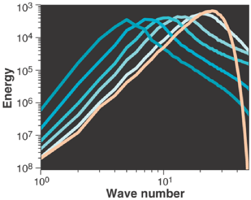
Figure 1: Magnetic energy spectra at different times (increasing roughly by a factor of 2). The curve with the right-most location of the peak corresponds to the initial time, while the other lines refer to later times (increasing from right to left). Note the propagation of spectral energy to successively smaller wavenumbers $k$, i.e. to successively larger scales. Adapted from Christensson et al. (2001).

In the non-decaying case, when the flow is driven by energy input at some forcing wavenumber $k_{\rm f}$, the inverse cascade is clearly seen if there is sufficient scale separation, i.e. if $k_{\rm f}$ is large compared with the smallest wavenumber $k_{1}$ that fits into a domain of size $L=2\pi/k_{1}$. An example is shown in Figure 2, where kinetic energy is injected at the wavenumber $k_{\rm f}=30k_{1}$. It is evident that there are two local maxima of spectral magnetic energy, one at the forcing wavenumber $k_{\rm f}$, and another one at a smaller wavenumber that we call $k_{\rm m}$, which is near $7k_{1}$ in Figure 2. During the kinematic stage the entire spectrum moves upward, with the spectral energy increasing at the same rate at all wavenumbers. Eventually, when the field has reached a certain level, the spectrum begins to change its shape and the second local maximum at $k_{\rm m}$ moves toward smaller values, suggestive of an inverse cascade. However, a more detailed analysis (Brandenburg 2001) shows that the energy transfer is nonlocal, i.e. most of the energy is transferred directly from the forcing wavenumber to the wavenumber where most of the mean field resides. This suggests that we have merely a nonlocal inverse transfer rather than a proper inverse cascade, where the energy transfer would be local in spectral space.

Figure 2: Magnetic energy spectra for a run with forcing at $k=30$. The times, in units of $(c_{\rm s}k_{1})^{-1}$, range from 0 (dotted line) to 10, 30, …, 290 (solid lines). The thick solid line gives the final state at $c_{\rm s}k_{1}t=1000$, corresponding to $u_{\rm rms}k_{\rm f}t\approx 2000$ turnover times. Here, $c_{\rm s}$ is the sound speed and $u_{\rm rms}$ is the turbulent rms velocity. Note that at early times the spectra peak at $k_{\max}\approx 7k_{1}$. The $k^{-1}$ and $k^{+3/2}$ slopes are given for orientation as dash-dotted lines. Adapted from Brandenburg (2001).

The position of the local maximum can readily be explained by mean-field dynamo theory with an $\alpha$ effect. The evolution equation of such a dynamo is

$${\partial\overline{\mbox{\boldmath$B$}}{}\over\partial t}=\mbox{\boldmath$\nabla$}{}\times\alpha\overline{\mbox{\boldmath$B$}}{}+\eta_{\rm T}\nabla^{2}\overline{\mbox{\boldmath$B$}}{},$$ (4)

where $\alpha$ is a pseudo-scalar, $\eta_{\rm T}=\eta+\eta_{\rm t}$ is the sum of microscopic Spitzer resistivity and turbulent resistivity, and an overbar denotes a suitably defined spatial average (e.g. planar average). Assuming $\overline{\mbox{\boldmath$B$}}{}=\hat{\bm{B}}_{\bm{k}}\exp(\lambda t+{\rm i}\bm{k}\cdot\bm{x})$ with eigenfunction $\hat{\bm{B}}_{\bm{k}}$, one finds the dispersion relation to be (Moffatt 1978)

$$\lambda(k)=|\alpha|k-\eta_{\rm T}k^{2},$$ (5)

where $k=|\bm{k}|$. The maximum growth rate is attained for a value of $k$ where ${\rm d}{}\lambda/{\rm d}{}k=0$, i.e. for $k=k_{\rm m}=\alpha/2\eta_{\rm T}$. The migration of the spectral maximum to smaller $k$ can then be explained as the result of a suppression of $\alpha$. In other words, as the dynamo saturates, $\alpha$ decreases, and so does $k_{\rm m}$, which corresponds to the spectral maximum moving to the left.

It should be noted that there is also the possibility of a suppression of $\eta_{\rm t}$, which would work the other way, so that this interpretation might not work. Indeed, there are arguments for a suppression of $\eta_{\rm t}$ that would be as strong as that of $\alpha$, but this applies only to the two-dimensional case and has to do with the conservation of the mean-squared vector potential in that case (Gruzinov & Diamond 1994). Simulations also find evidence that in three dimensions the suppression of $\alpha$ is stronger than that of $\eta_{\rm t}$ (Brandenburg et al. 2008b).

In the following we discuss in detail the role played by magnetic helicity. This has been reviewed extensively in the last few years (Ji & Prager 2002, Brandenburg & Subramanian 2005, Blackman & Ji 2006).

3 Slow saturation

In a closed or periodic domain, the saturation of a helical large-scale dynamo is found to be resistively slow and the final field strength is reached with a time behavior of the form (Brandenburg 2001)

$$\langle\overline{\mbox{\boldmath$B$}}{}^{2}\rangle(t)=B_{\rm eq}^{2}{k_{\rm m}\over k_{\rm f}}\left[1-e^{-2\eta k_{\rm m}^{2}(t-t_{\rm s})}\right]\quad\mbox{for $t>t_{\rm s}$},$$ (6)

where $B_{\rm eq}$ is the equipartition field strength and $t_{\rm s}$ is the time when the slow saturation phase begins. We emphasize that it is the microscopic $\eta$ that enters Equation (6), and that the relevant length scale, $2\pi/k_{\rm m}$, is that of the large-scale field, so the saturation behavior is truly very slow.

The reason for this slow saturation behavior is related to the conservation of magnetic helicity, which obeys the evolution equation (e.g., Ji et al. 1995, Ji 1999)

$${{\rm d}{}\over{\rm d}{}t}\langle\mbox{\boldmath$A$}{}\cdot\mbox{\boldmath$B$}{}\rangle=-2\eta\mu_{0}\langle\mbox{\boldmath$J$}{}\cdot\mbox{\boldmath$B$}{}\rangle-\langle\mbox{\boldmath$\nabla$}{}\cdot\mbox{\boldmath$F$}{}_{\rm H}\rangle.$$ (7)

where $\mbox{\boldmath$F$}{}_{\rm H}$ is the magnetic helicity flux, but for the periodic domain under consideration we have $\mbox{\boldmath$\nabla$}{}\cdot\mbox{\boldmath$F$}{}_{\rm H}=0$. Clearly, in the final state we have then $\langle\mbox{\boldmath$J$}{}\cdot\mbox{\boldmath$B$}{}\rangle=0$. This can only be satisfied for nontrivial helical fields if small-scale and large-scale fields have values of opposite sign, but equal magnitude, i.e. $\langle\mbox{\boldmath$j$}{}\cdot\mbox{\boldmath$b$}{}\rangle=-\langle\overline{\mbox{\boldmath$J$}}{}\cdot\overline{\mbox{\boldmath$B$}}{}\rangle$, where $\mbox{\boldmath$B$}{}=\overline{\mbox{\boldmath$B$}}{}+\mbox{\boldmath$b$}{}$ and $\mbox{\boldmath$J$}{}=\overline{\mbox{\boldmath$J$}}{}+\mbox{\boldmath$j$}{}$ are the decompositions of magnetic field and current density into mean and fluctuating parts. Here we choose to define mean fields as one- or two-dimensional coordinate averages. Examples include planar averages such as $xy$, $yz$, or $xz$ averages in a periodic Cartesian domain, as well as one-dimensional averages such as $y$ or $\phi$ averages in Cartesian or spherical domains, $(r,\theta,\phi)$, where the other two directions are non-periodic.

Equation (6) can be derived under the assumption that large-scale and small-scale fields are fully helical with $\overline{\mbox{\boldmath$J$}}{}\cdot\overline{\mbox{\boldmath$B$}}{}=k_{\rm m}^{2}\overline{\mbox{\boldmath$A$}}{}\cdot\overline{\mbox{\boldmath$B$}}{}=\mp k_{\rm m}\overline{\mbox{\boldmath$B$}}{}^{2}$ and $\langle\mbox{\boldmath$j$}{}\cdot\mbox{\boldmath$b$}{}\rangle=\pm k_{\rm f}\langle\mbox{\boldmath$b$}{}^{2}\rangle\approx\pm k_{\rm f}B_{\rm eq}^{2}$, where upper and lower signs refer to positive and negative helicity of the small-scale turbulence and we have assumed that the small-scale field has already reached saturation, i.e. $\langle\mbox{\boldmath$b$}{}^{2}\rangle\approx B_{\rm eq}^{2}\equiv\mu_{0}\langle\rho\mbox{\boldmath$u$}{}^{2}\rangle$, where $\rho$ is the density and $\mbox{\boldmath$u$}{}=\mbox{\boldmath$U$}{}-\overline{\bm{U}}$ is the fluctuating velocity.

A mean-field theory that obeys magnetic helicity conservation was originally developed by Kleeorin & Ruzmaikin (1982) and has recently been applied to explaining slow saturation (Field & Blackman 2002, Blackman & Brandenburg 2002, Subramanian 2002). The main idea is that the $\alpha$ effect has two contributions (Pouquet et al. 1976),

$$\alpha=\alpha_{\it K}+\alpha_{\it M},$$ (8)

where $\alpha_{\it K}=-{\textstyle{1\over 3}}\tau\overline{\mbox{\boldmath$\omega$}{}\cdot\mbox{\boldmath$u$}{}}$ is the usual kinetic $\alpha$ effect related to the kinetic helicity, with $\mbox{\boldmath$\omega$}{}=\mbox{\boldmath$\nabla$}{}\times\mbox{\boldmath$u$}{}$ being the vorticity, and $\alpha_{\it M}={\textstyle{1\over 3}}\tau\overline{\mbox{\boldmath$j$}{}\cdot\mbox{\boldmath$b$}{}}/\rho_{0}$ is a magnetic $\alpha$ effect that can, for example, be produced by the growing magnetic field in an attempt to conserve magnetic helicity. (Here, $\rho_{0}$ is an average density, but we note that there is at present no adequate theory for compressible systems with nonuniform density.)

Note that $\alpha_{\it M}$ is related to the small-scale current helicity and hence to the small-scale magnetic helicity which, in turn, obeys an evolution equation similar to Equation (7), but with an additional production term, $2\overline{\mbox{\boldmath${\cal E}$}}{}\cdot\overline{\mbox{\boldmath$B$}}{}$, that arises from mean-field theory via $\overline{\mbox{\boldmath${\cal E}$}}{}=\alpha\overline{\mbox{\boldmath$B$}}{}-\eta_{\rm t}\mu_{0}\overline{\mbox{\boldmath$J$}}{}$, and thus from the $\alpha$ effect itself. The equation for $\alpha_{\it M}$ has then the form

$${\partial\alpha_{\it M}\over\partial t}=-2\eta_{\rm t}k_{\rm f}^{2}\left({\overline{\mbox{\boldmath${\cal E}$}}{}\cdot\overline{\mbox{\boldmath$B$}}{}\over B_{\rm eq}^{2}}+{\alpha_{\it M}\over R_{\rm m}}\right)-\mbox{\boldmath$\nabla$}{}\cdot\overline{\mbox{\boldmath$F$}}{}_{\alpha},$$ (9)

where $R_{\rm m}=\eta_{\rm t}/\eta$ is a measure of the ratio of turbulent to microscopic magnetic diffusivity. With $\eta_{\rm t}=u_{\rm rms}/3k_{\rm f}$ (Sur et al. 2008) we can relate this to the more usual definition for the magnetic Reynolds number, $\tilde{R}_{\rm m}=u_{\rm rms}/\eta k_{\rm f}$, via $\tilde{R}_{\rm m}=3R_{\rm m}$. Furthermore, we have allowed for the possibility of fluxes of magnetic and current helicities that also lead to a flux of $\alpha_{\it M}$. Such fluxes are primarily important in inhomogeneous domains and especially in open domains where one can have an outward helicity flux (Ji 1999).

The use of Equation (8) is sometimes criticized because it is based on a closure assumption. Indeed, there are questions regarding the meaning of the term $\overline{\mbox{\boldmath$j$}{}\cdot\mbox{\boldmath$b$}{}}$ and whether it really applies to the actual field, or the field in the unquenched case. This has been discussed in detail in a critical paper by Rädler & Rheinhardt (2007). Part of this ambiguity can already be clarified in the low conductivity limit. Sur et al. (2007) have shown that one can express $\alpha$ either completely in terms of the helical properties of the velocity field or, alternatively, as the sum of two terms, a so-called kinetic $\alpha$ effect and an oppositely signed term proportional to the helical part of the small scale magnetic field. However, it is fair to say that the problem is not yet completely understood. The strongest argument in favor of Equations (8) and (9) is that they reproduce catastrophic (i.e. $R_{\rm m}$-independent) quenching of $\alpha$ and that this approach has led to the prediction that such quenching can be alleviated by magnetic helicity fluxes. This prediction has subsequently been tested successfully on various occasions (Brandenburg 2005, Käpylä et al. 2008). Finally, it should be noted that Equation (8) has also been confirmed directly using turbulence simulations (Brandenburg et al. 2005c, 2007).

The idea to model dynamo saturation and suppression of $\alpha$ by solving a dynamical equation for $\alpha_{\it M}$ is called dynamical quenching. In addition to the resistively slow saturation behavior described by Equation (6), this approach has also been applied to decaying turbulence with helicity (Yousef et al. 2003; Blackman & Field 2004), where the conservation of magnetic helicity results in a slow-down of the decay. This can be modeled by an $\alpha$ effect that offsets the turbulent decay proportional to $\eta_{\rm t}k^{2}$ such that the decay rate becomes nearly equal to the resistive value, $\eta k^{2}$. This is explained in detail in the following section.

4 Decay in a Cartesian domain

In the context of driven turbulence, the properties of solutions of a decaying helical magnetic field were studied earlier by Yousef et al. (2003), who found that for fields with $\overline{\mbox{\boldmath$B$}}{}^{2}/B_{\rm eq}^{2}\mathrel{\mathchoice{\vbox{\offinterlineskip\halign{\hfil$\displaystyle#$\hfil\cr>\cr\sim\cr}}}{\vbox{\offinterlineskip\halign{\hfil$\textstyle#$\hfil\cr>\cr\sim\cr}}}{\vbox{\offinterlineskip\halign{\hfil$\scriptstyle#$\hfil\cr>\cr\sim\cr}}}{\vbox{\offinterlineskip\halign{\hfil$\scriptscriptstyle#$\hfil\cr>\cr\sim\cr}}}}R_{\rm m}^{-1}$ the decay of $\overline{\mbox{\boldmath$B$}}{}$ is slowed down and can quantitatively be described by the dynamical quenching model. This model applies even to the case where the turbulence is nonhelical and where there is initially no $\alpha$ effect in the usual sense. However, the magnetic contribution to $\alpha$ is still non-vanishing, because the $\alpha_{\it M}$ term is driven by the helicity of the large-scale field.

To demonstrate this quantitatively, Yousef et al. (2003) have adopted a one-mode approximation with $\overline{\mbox{\boldmath$B$}}{}=\hat{\bm{B}}(t)\exp({\rm i}k_{1}z)$, and used the mean-field induction equation together with the dynamical $\alpha$-quenching formula (9),

$${{\rm d}{}\hat{\bm{B}}\over{\rm d}{}t}={\rm i}\bm{k}_{1}\times\hat{\mbox{\boldmath${\cal E}$}{}}-\eta k_{1}^{2}\hat{\bm{B}},$$ (10)

$${{\rm d}{}\alpha\over{\rm d}{}t}=-2\eta_{\rm t}k_{\rm f}^{2}\left({{\rm Re}(\hat{\mbox{\boldmath${\cal E}$}{}}^{*}\cdot\hat{\bm{B}})\over B_{\rm eq}^{2}}+{\alpha\over R_{\rm m}}\right),$$ (11)

where the flux term is neglected, $\hat{\mbox{\boldmath${\cal E}$}{}}=\alpha\hat{\bm{B}}-\eta_{\rm t}{\rm i}\bm{k}_{1}\times\hat{\bm{B}}$ is the electromotive force, and $\bm{k}_{1}=(0,0,k_{1})$.

Figure 3: Dynamical quenching model with helical and nonhelical initial fields, and an additional $\eta_{\rm t}$ quenching function, $\eta_{\rm t}=\eta_{\rm t0}/(1+\tilde{g}|\overline{\mbox{\boldmath$B$}}{}|/B_{\rm eq})$. The quenching parameters are $\tilde{g}=0$ (solid line) and 3 (dotted line). The graph for the nonhelical cases has been shifted in $t$ so that one sees that the decay rates are asymptotically equal at late times. The value of $\eta_{\rm T}$ used to normalize the abscissa is based on the unquenched value. Adapted from Yousef et al. (2003).

Figure 3 compares the evolution of $\overline{\mbox{\boldmath$B$}}{}/B_{\rm eq}$ for helical and nonhelical initial conditions, $\hat{\bm{B}}\propto(1,{\rm i},0)$ and $\hat{\bm{B}}\propto(1,0,0)$, respectively. In the case of a nonhelical field, the decay rate is not quenched at all, but in the helical case quenching sets in for $\overline{\mbox{\boldmath$B$}}{}^{2}/B_{\rm eq}^{2}\mathrel{\mathchoice{\vbox{\offinterlineskip\halign{\hfil$\displaystyle#$\hfil\cr>\cr\sim\cr}}}{\vbox{\offinterlineskip\halign{\hfil$\textstyle#$\hfil\cr>\cr\sim\cr}}}{\vbox{\offinterlineskip\halign{\hfil$\scriptstyle#$\hfil\cr>\cr\sim\cr}}}{\vbox{\offinterlineskip\halign{\hfil$\scriptscriptstyle#$\hfil\cr>\cr\sim\cr}}}}R_{\rm m}^{-1}$. The onset of quenching at $\overline{\mbox{\boldmath$B$}}{}^{2}/B_{\rm eq}^{2}\approx R_{\rm m}^{-1}$ is well reproduced by the simulation. In the nonhelical case, however, some weaker form of quenching sets in when $\overline{\mbox{\boldmath$B$}}{}^{2}/B_{\rm eq}^{2}\approx 1$. We refer to this as standard quenching (e.g. Kitchatinov et al. 1994) which is known to be always present; see Equation (6). Blackman & Brandenburg (2002) found that, for a range of different values of $R_{\rm m}$, $\tilde{g}=3$ results in a good description of the simulations of cyclic $\alpha\Omega$-type dynamos that were reported by Brandenburg et al. (2002.).

5 Relevance to the reversed field pinch

The dynamical quenching approach has been applied to modeling the dynamics of the reversed field pinch, where one has an initially helical magnetic field of the form

$$\overline{\mbox{\boldmath$B$}}{}=\hat{\bm{B}}\pmatrix{0\cr J_{1}(kr)\cr J_{0}(kr)},$$ (12)

where we have adopted cylindrical coordinates $(r,\theta,z)$. In a cylinder of radius $R$ such an initial field becomes kink unstable when $kR\mathrel{\mathchoice{\vbox{\offinterlineskip\halign{\hfil$\displaystyle#$\hfil\cr>\cr\sim\cr}}}{\vbox{\offinterlineskip\halign{\hfil$\textstyle#$\hfil\cr>\cr\sim\cr}}}{\vbox{\offinterlineskip\halign{\hfil$\scriptstyle#$\hfil\cr>\cr\sim\cr}}}{\vbox{\offinterlineskip\halign{\hfil$\scriptscriptstyle#$\hfil\cr>\cr\sim\cr}}}}\pi$. Both laboratory measurements (e.g. Caramana & Baker 1984) and numerical simulations (Ho et al. 1989) confirm the idea that the field-aligned current leads to kink instability, and hence to small-scale turbulence and thereby to the emergence of $\eta_{\rm t}$ and $\alpha$.

Figure 4: Time evolution of toroidal flux in the RFP experiment of Caramana & Baker (1984) compared with a calculation with no dynamo effect. The decay around $t=18$ms is due to termination of the applied electric field. Courtesy of E. J. Caramana and D. A. Baker.

Just as in the case discussed in Section 4, the emergence of $\alpha$ slows down the decay in such a way that the toroidal field remains nearly constant and is maintained against resistive decay; see Figure 4. The details of this mechanism have been discussed by Ji & Prager (2002). In particular, they show that the parallel electric field cannot be balanced by the resistive term alone, and that there must be an additional component resulting from small-scale correlations of velocity and magnetic field, $\overline{\mbox{\boldmath$u$}{}\times\mbox{\boldmath$b$}{}}$, that explain the observed profiles of mean electric field and mean current density. Furthermore, the parallel electric field reverses sign near the edge of the device, while the parallel current density does not. Again, this can only be explained by additional contributions from small-scale correlations of velocity and magnetic field. The RFP experiment also shows that magnetic helicity evolves on time scales faster than the resistive scale, which is only compatible with the presence of a finite magnetic helicity flux divergence (Ji et al. 1995, Ji 1999).

6 Magnetic helicity in realistic dynamos

Astrophysical dynamos saturate and evolve on dynamical time scales and are thus not resistively slow. Current research shows that this can be achieved by expelling magnetic helicity from the domain through helicity fluxes. This is why we have allowed for the $\mbox{\boldmath$\nabla$}{}\cdot\overline{\mbox{\boldmath$F$}}{}_{\alpha}$ term in Equation (9). Since the magnetic $\alpha$ effect is proportional to the current helicity of the fluctuating field, the $\overline{\mbox{\boldmath$F$}}{}_{\alpha}$ flux should be proportional to the current helicity flux of the fluctuating field.

The presence of the flux term generally lowers the value of $|\alpha_{\it M}|$, and since the $\alpha_{\it M}$ term quenches the total value of $\alpha$ ($=\alpha_{\it K}+\alpha_{\it M}$), the effect of this helicity flux is to alleviate an otherwise catastrophic quenching. Indeed, in an open domain and without a flux divergence, the $\alpha_{\it M}/R_{\rm m}$ term in Equation (9) can result in “catastrophically low” saturation field strengths that are by a factor $R_{\rm m}^{1/2}$ smaller than the equipartition field strength (Gruzinov & Diamond 1994; Brandenburg & Subramanian 2005b).

Magnetic helicity obeys a conservation law and is therefore conceptually easier to tackle than current helicity. However, there is the difficulty of gauge dependence of magnetic helicity density and its flux. It is therefore safer to work with the current helicity, which is also the quantity that enters in Equations (8) and (9). However, more work needs to be done to establish the connection between the two approaches.

Over the past 10 years there has been mounting evidence that the Sun sheds magnetic helicity (and hence current helicity) through coronal mass ejections and other events. Understanding the functional form of such fluxes is very much a matter of ongoing research (Subramanian & Brandenburg 2004, 2006, Brandenburg et al. 2009). In the following section we present a simple calculation that allows us to estimate the amount of magnetic helicity losses required for the solar dynamo to work.

7 Estimating the required magnetic helicity losses

In order to estimate the magnetic helicity losses required to alleviate catastrophic quenching we make use of the relation between the $\alpha$ effect and the divergence of the current helicity flux (Brandenburg & Subramanian 2005a),

$$\alpha={\alpha_{\it K}+R_{\rm m}\left[\eta_{\rm t}\mu_{0}\overline{\mbox{\boldmath$J$}}{}\cdot\overline{\mbox{\boldmath$B$}}{}/B_{\rm eq}^{2}-\mbox{\boldmath$\nabla$}{}\cdot\overline{\mbox{\boldmath$F$}}{}_{\rm C}/(2k_{\rm f}^{2}B_{\rm eq}^{2})-\dot{\alpha}/(2\eta_{\rm t}k_{\rm f}^{2})\right]\over 1+R_{\rm m}\overline{\mbox{\boldmath$B$}}{}^{2}/B_{\rm eq}^{2}},$$ (13)

where $\dot{\alpha}=\partial\alpha/\partial t$ and $\overline{\mbox{\boldmath$F$}}{}_{\rm C}$ is the mean flux of current helicity from the small-scale field, $\overline{(\mbox{\boldmath$\nabla$}{}\times\mbox{\boldmath$e$}{})\times(\mbox{\boldmath$\nabla$}{}\times\mbox{\boldmath$b$}{})}$, where $e$ is the fluctuating component of the electric field; see also Subramanian & Brandenburg (2004). In the steady-state limit and at large $R_{\rm m}$ we have

$$\alpha\approx\eta_{\rm t}{\mu_{0}\overline{\mbox{\boldmath$J$}}{}\cdot\overline{\mbox{\boldmath$B$}}{}\over\overline{\mbox{\boldmath$B$}}{}^{2}}-{\mbox{\boldmath$\nabla$}{}\cdot\overline{\mbox{\boldmath$F$}}{}_{\rm C}\over 2k_{\rm f}^{2}\overline{\mbox{\boldmath$B$}}{}^{2}}.$$ (14)

We neglect the $\overline{\mbox{\boldmath$J$}}{}\cdot\overline{\mbox{\boldmath$B$}}{}$ term, because the catastrophic quenching in dynamos with boundaries has never been seen to be alleviated by this term (Brandenburg & Subramanian 2005b). Thus, we use Equation (14) to estimate $\mbox{\boldmath$\nabla$}{}\cdot\overline{\mbox{\boldmath$F$}}{}_{\rm C}$ as

$$\mbox{\boldmath$\nabla$}{}\cdot\overline{\mbox{\boldmath$F$}}{}_{\rm C}=2\alpha k_{\rm f}^{2}\overline{\mbox{\boldmath$B$}}{}^{2}.$$ (15)

Next, we take the volume integral over one hemisphere, i.e.

$${\cal L}_{\rm C}\equiv\oint_{2\pi}\overline{\mbox{\boldmath$F$}}{}_{\rm C}\cdot{\rm d}{}\mbox{\boldmath$S$}{}=\int\mbox{\boldmath$\nabla$}{}\cdot\overline{\mbox{\boldmath$F$}}{}_{\rm C}\,{\rm d}{}V={2\pi\over 3}R^{3}\langle 2\alpha k_{\rm f}^{2}\overline{\mbox{\boldmath$B$}}{}^{2}\rangle,$$ (16)

where ${\cal L}_{\rm C}$ is the “luminosity” or “power” of current helicity. We estimate $\langle\alpha\rangle$ using $\alpha\Omega$ dynamo theory which predicts that (e.g., Robinson & Durney 1982, see also Brandenburg & Subramanian 2005a)

$$\alpha k_{1}\Delta\Omega\approx\omega_{\rm cyc}^{2},$$ (17)

where $\omega_{\rm cyc}=2\pi/T_{\rm cyc}$ is the cycle frequency of the dynamo, $T_{\rm cyc}$ is the 22 year cycle period of the Sun, $\alpha$ is assumed constant over each hemisphere, and $\Delta\Omega$ is the total latitudinal shear, i.e. about $0.3\Omega$ for the Sun. There is obviously an uncertainty in relating local values of $\alpha$ to volume averages. However, if we do set the two equal, we obtain at least an upper limit for ${\cal L}_{\rm C}$. We may then relate this to the luminosity of magnetic helicity, ${\cal L}_{\rm H}$, that we assume to be proportional to ${\cal L}_{\rm C}$ via

$${\cal L}_{\rm C}=k_{\rm f}^{2}{\cal L}_{\rm H}.$$ (18)

With this we find for the total magnetic helicity loss over half a cycle (one 11 year cycle)

$${\textstyle{1\over 2}}{\cal L}_{\rm H}T_{\rm cyc}\leq{4\pi\over 3}R^{3}{\omega_{\rm cyc}^{2}\over k_{1}\Delta\Omega}T_{\rm cyc}\langle\overline{\mbox{\boldmath$B$}}{}^{2}\rangle={4\pi\over 3}LR^{3}{\omega_{\rm cyc}\over\Delta\Omega}\langle\overline{\mbox{\boldmath$B$}}{}^{2}\rangle,$$ (19)

where we have estimated $k_{1}=2\pi/L$ for the relevant wavenumber of the dynamo in terms of the thickness of the convection zone $L$. Inserting now values relevant for the Sun, $L=200\,{\rm Mm}$, $R=700\,{\rm Mm}$, $\omega_{\rm cyc}/\Delta\Omega=10^{-2}$, and $\overline{\mbox{\boldmath$B$}}{}\sim 300\,{\rm G}$, we obtain

$${\textstyle{1\over 2}}{\cal L}_{\rm H}T_{\rm cyc}\leq 10^{46}\,{\rm Mx}^{2}/\mbox{cycle}.$$ (20)

This is comparable to earlier estimates based partly on observations (Berger & Ruzmaikin 2000; DeVore 2000) and partly on turbulence simulations (Brandenburg & Sandin 2004), but we recall that Equation (20) is only an upper limit. Furthermore, the connection between current helicity and magnetic helicity assumed in relation (18) is quite rough and has only been seriously confirmed under isotropic conditions. In addition, it is not clear that the gauge-invariant magnetic helicity flux defined by Berger & Field (1984) and Finn & Antonsen (1985) is actually the quantity of interest. Following earlier work of Subramanian & Brandenburg (2006), the gauge-invariant magnetic helicity is not in any obvious way related to the current helicity which, in turn, is related to the density of the flux linking number and is at least approximately equal to the magnetic helicity in the Coulomb gauge.

In summary, although magnetic helicity is conceptually advantageous in that it obeys a conservation equation, the difficulty in dealing with a gauge-dependent quantity can be quite serious. Moreover, as emphasized before, it is really the current helicity that is primarily of interest, so it would be useful to shift attention from magnetic helicity fluxes to current helicity fluxes.

8 Conclusions

In this review we have attempted to highlight the importance of magnetic helicity in modern nonlinear dynamo theory. Much of the early work on the reversed field pinch since the mid 1980s now proves to be extremely relevant in view of the possibility of resistively slow saturation by a self-inflicted build-up of small-scale current helicity, $\overline{\mbox{\boldmath$j$}{}\cdot\mbox{\boldmath$b$}{}}$, as the dynamo produces large-scale current helicity, $\overline{\mbox{\boldmath$J$}}{}\cdot\overline{\mbox{\boldmath$B$}}{}$. Since this concept is not yet universally accepted, the additional evidence from the reversed field pinch experiment can be quite useful.

The interpretation of resistively slow saturation has led to the proposed solution that magnetic helicity fluxes (or current helicity fluxes) are responsible for removing excess small-scale magnetic helicity from the system. This allows the dynamo to reach saturation levels that can otherwise be $R_{\rm m}^{1/2}$ times smaller than the equipartition value given by the kinetic energy density of the turbulent motions. The consequences of this prediction have been tested in direct simulations (Fig. 3 of Brandenburg 2005 and Fig. 17 of Käpylä et al. 2008), confirming thereby ultimately basic aspects of incorporating the magnetic helicity equation into mean-field models. However, more progress is needed in addressing questions regarding the relative importance of magnetic and current helicity fluxes through the surface compared to diffusive fluxes across the equator (Brandenburg et al. 2009).

We reiterate that the reversed field pinch experiment is not directly relevant to the self-excited dynamo, but rather its nonlinear saturation mechanism. So far, successful self-excited dynamo experiments have only been performed with liquid sodium (Gailitis et al. 2000; Stieglitz & Müller 2001; Monchaux et al. 2007). This may change in future given that one can usually achieve much higher magnetic Reynolds numbers in plasmas than in liquid metals (Spence et al. 2009). It might then, for the first time, be possible to address experimentally questions regarding the relative importance of magnetic and current helicity fluxes for dynamos.

Acknowledgments

I thank the referees for detailed and constructive comments that have helped to improve the presentation. This work was supported in part by the Swedish Research Council, grant 621-2007-4064, and the European Research Council under the AstroDyn Research Project 227952.

References

References

- [1] Batchelor, G. K. 1950, Proc. Roy. Soc. Lond., A201, 405
- [2] Berger, M., & Field, G. B. 1984, J. Fluid Mech., 147, 133
- [3] Berger, M., & Ruzmaikin, A. 2000, J. Geophys. Res., 105, 10481
- [4] Blackman, E. G., & Brandenburg, A. 2002, ApJ, 579, 359
- [5] Blackman, E. G., & Field, G. B. 2004, Phys. Plasmas, 11, 3264
- [6] Blackman, E. G., & Ji, H. 2006, MNRAS, 369, 1837
- [7] Brandenburg, A. 2001, ApJ, 550, 824
- [8] Brandenburg, A. 2005, ApJ, 625, 539
- [9] Brandenburg, A., & Sandin, C. 2004, A&A, 427, 13
- [10] Brandenburg, A., & Subramanian, K. 2005a, Phys. Rep., 417, 1
- [11] Brandenburg, A., & Subramanian, K. 2005b, Astron. Nachr., 326, 400
- [12] Brandenburg, A., & Subramanian, K. 2005c, A&A, 439, 835
- [13] Brandenburg, A., & Subramanian, K. 2007, Astron. Nachr., 328, 507
- [14] Brandenburg, A., Rädler, K.-H., Rheinhardt, M., & Käpylä, P. J. 2008a, ApJ, 676, 740
- [15] Brandenburg, A., Rädler, K.-H., Rheinhardt, M., & Subramanian, K. 2008b, ApJ, 687, L49
- [16] Brandenburg, A., Candelaresi, S., & Chatterjee, P. 2009, MNRAS, 398, 1414
- [17] Brandenburg, A., Dobler, W., & Subramanian, K. 2002, Astron. Nachr., 323, 99
- [18] Caramana, E.J., & Baker, D.A. 1984, Nuclear Fusion, 24, 423
- [19] Christensson, M., Hindmarsh, M., & Brandenburg, A. 2001, Phys. Rev. E, 64, 056405
- [20] Cho, J., Lazarian, A., & Vishniac, E. 2002, ApJ, 564, 291
- [21] Cowling, T. G. 1933, MNRAS, 94, 39
- [22] DeVore, C. R. 2000, ApJ, 539, 944
- [23] Field, G. B., & Blackman, E. G. 2002, ApJ, 572, 685
- [24] Finn, J. M., & Antonsen, T. M. 1985, Comments Plasma Phys. Controlled Fusion, 9, 111123
- [25] Frisch, U., Pouquet, A., Léorat, J., & Mazure, A. 1975, J. Fluid Mech., 68, 769
- [26] Gailitis, A., Lielausis, O., Platacis, E., Dement’ev, S., Cifersons, A., Gerbeth, G., Gundrum, T., Stefani, F., Christen, M., & Will, G. 2001, Phys. Rev. Lett., 86, 3024
- [27] Gruzinov, A. V., & Diamond, P. H. 1994, Phys. Rev. Lett., 72, 1651
- [28] Haugen, N. E. L., Brandenburg, A., & Dobler, W. 2003, ApJ, 597, L141
- [29] Herzenberg, A. 1958, Proc. Roy. Soc. Lond., 250A, 543
- [30] Ho, Y. L., Prager, S. C., & Schnack, D. D. 1989, Phys. Rev. Lett., 62, 1504
- [31] Ji, H. 1999, Phys. Rev. Lett., 83, 3198
- [32] Ji, H., & Prager, S. C. 2002, Magnetohydrodynamics, 38, 191
- [33] Ji, H., Prager, S. C., & Sarff, J. S. 1995, Phys. Rev. Lett., 74, 2945
- [34] Käpylä, P. J., Korpi, M. J., & Brandenburg, A. 2008, A&A, 491, 353
- [35] Kazantsev, A. P. 1968, Sov. Phys. JETP, 26, 1031
- [36] Kitchatinov, L. L., Rüdiger, G., & Pipin, V. V. 1994, Astron. Nachr., 315, 157
- [37] Kleeorin, N. I., & Ruzmaikin, A. A. 1982, Magnetohydrodynamics, 18, 116
- [38] Kraichnan, R. H. 1976, J. Fluid Mech., 75, 657
- [39] Larmor, J. 1919, Rep. Brit. Assoc. Adv. Sci., 159,
- [40] Larmor, J. 1934, MNRAS, 94, 469
- [41] Meneguzzi, M., Frisch, U., & Pouquet, A. 1981, Phys. Rev. Lett., 47, 1060
- [42] Moffatt, H. K. 1978, Magnetic field generation in electrically conducting fluids (Cambridge University Press, Cambridge), pp. 175–178
- [43] Monchaux, R., Berhanu, M., Bourgoin, M., Moulin, M., Odier, Ph., Pinton, J. -F., Volk, R., Fauve, S., Mordant, N., Petrelis, F., Chiffaudel, A., Daviaud, F., Dubrulle, B., Gasquet, C., Marie, L., & Ravelet, F. 2007, Phys. Rev. Lett., 98, 044502
- [44] Ortolani, S., & Schnack, D. D. 1993, Magnetohydrodynamics of plasma relaxation (World Scientific, Singapore)
- [45] Parker, E. N. 1955, ApJ, 122, 293
- [46] Pouquet, A., Frisch, U., & Léorat, J. 1976, J. Fluid Mech., 77, 321
- [47] Proctor, M. R. E. 2007, MNRAS, 382, L39
- [48] Rädler K.-H., Rheinhardt M. 2007, Geophys. Astrophys. Fluid Dyn., 101, 11
- [49] Robinson, R. D., & Durney, B. R. 1982, A&A, 108, 322
- [50] Rogachevskii, I., & Kleeorin, N. 2003, Phys. Rev. E, 68, 036301
- [51] Schekochihin, A. A., Maron, J. L., Cowley, S. C., & McWilliams, J. C. 2002, ApJ, 576, 806
- [52] Spence, E. J., Reuter, K., & Forest, C. B. 2009, ApJ, 700, 470
- [53] Stieglitz, R., & Müller, U. 2001, Phys. Fluids, 13, 561
- [54] Subramanian, K. 2002, Bull. Astr. Soc. India, 30, 715
- [55] Subramanian, K., & Brandenburg, A. 2004, Phys. Rev. Lett., 93, 205001
- [56] Subramanian, K., & Brandenburg, A. 2006, ApJ, 648, L71
- [57] Sur, S., Subramanian, K., & Brandenburg, A. 2007, MNRAS, 376, 1238
- [58] Sur, S., Brandenburg, A., & Subramanian, K. 2008, MNRAS, 385, L15
- [59] Vishniac, E. T., & Brandenburg, A. 1997, ApJ, 475, 263
- [60] Yousef, T. A., Brandenburg, A., & Rüdiger, G. 2003, A&A, 411, 321