The Second-Order Talbot Effect with Entangled Photon Pairs

Abstract

The second-order Talbot effect is analyzed for a periodic object illuminated by entangled photon pairs in both the quantum imaging and quantum lithography configurations. The Klyshko picture is applied to describe the quantum imaging scheme, in which self-images of the object that may or may not be magnified can be observed nonlocally in the photon coincidences but not in the singles count rate. In the quantum lithography setup, we find that the second-order Talbot length is half that of the classical first-order case, thus the resolution may be improved by a factor of two.

I Introduction

Classical image formation is most commonly associated with some type of lens, with the exception of the earliest means of imaging known to mankind, the pinhole camera. A less familiar form of lensless imaging, in which a periodic structure can produce self-images at certain regular distances, was first discovered by Talbot Talbot in 1836, partially explained by Rayleigh Rayleigh in 1881, and further explored by Weisel Weisel and Wolfke Wolfke early in the last century. The observation in recent years of this self-image replication in several new areas of research has led to renewed interest in this remarkable phenomenon, which contains much physics still unexplored.

The Talbot effect is a near field diffraction phenomenon in which a plane wave transmitted through a grating or other periodic structure propagates in such a way that the grating structure is replicated at multiples of a certain longitudinal distance. Rayleigh explained it as a natural consequence of Fresnel diffraction and the interference of the diffracted beams Rayleigh ; he showed analytically that for plane wave illumination the self-images repeat at multiples of the Talbot length $z_{\textrm{\tiny}{T}}=2a^{2}/\lambda$, where $a$ is the period of the grating and $\lambda$ the wavelength of the incident light. At half-integral multiples, the self-images are laterally shifted by half a period, and at intermediate distances of $z=(p/q)z_{\textrm{\tiny}{T}}$, where $p$ and $q$ are integers with no common factor, the images have a smaller period of $a/n$ ($n=2,3,4,\ldots$). These diffraction images are in fact a superimposition of shifted and complex weighted replicas of the original object Winthrop .

Potential applications of the Talbot effect have been found in image processing and synthesis, photolithography, optical testing, optical metrology and spectrometry Patorski . The effect is also well known in the field of acousto-optics, electron optics and electron microscopy Cowley . Recently, it has also been demonstrated in atomic waves Chapman ; Wu , Bose-Einstein condensates Deng ; Li , large C₇₀ fullerene molecules Brezger , waveguide arrays Iwanow , and X-ray phase imaging Weitkamp .

However, all the above demonstrations involved the first-order field intensity. In recent years, second-order (or two-photon) correlation intensity measurements have led to the discovery of many new, formerly unexpected phenomena. The first demonstration of “ghost” imaging and interference was performed by Shih’s group in the mid 1990’s, who exploited the spatial correlation of entangled photon pairs generated from spontaneous parametric down conversion (SPDC) Pittman ; Strekalov . In ghost imaging, an image of an object in the signal path to one detector is observed in the coincidence counts with another detector in the idler arm, if the Gaussian “two-photon” thin lens equation is satisfied. A scheme with both signal and idler beams in a Bessel beam mode was suggested by Vidal et al. to demonstrate conditional interference patterns in the second-order correlation function Vidal . In this paper we also exploit the transverse correlations of entangled photon pairs from SPDC, and present a general analysis of the second-order Talbot effect using the Klyshko advanced-wave picture Klyshko . It will be shown that self-images of a periodic structure can be nonlocally observed in the two-photon coincidence count measurement but not in the singles counts. Although spatially periodic objects represent only a subgroup of all objects that can generate self-images, they are still of fundamental importance and may reveal interesting new physics.

II Two-photon Talbot Effect

II.1 Talbot effect in quantum imaging

Let us first briefly review two-photon (biphoton) optics. From Glauber’s quantum measurement theory, the two-photon coincidence counting rate for two point photodetectors is given by Goodman

$$R_{cc}=\frac{1}{T}\int^{T}_{0}dt_{1}\int^{T}_{0}dt_{2}|\Psi(\vec{r}_{1},t_{1};\vec{r}_{2},t_{2})|^{2},$$ (1)

where the two-photon or biphoton amplitude $\Psi$ is determined by the matrix element between the vacuum state $|0\rangle$ and the two-photon state $|\psi\rangle$

$$\Psi(\vec{r}_{1},t_{1};\vec{r}_{2},t_{2})=\langle 0|E^{(+)}_{1}(\vec{r}_{1},t_{1})E^{(+)}_{2}(\vec{r}_{2},t_{2})|\psi\rangle.$$ (2)

Here $E^{(+)}_{j}(\vec{r}_{j},t_{j})$ $(j=1,2)$ is the positive frequency part of the electric field at point $\vec{r}_{j}$ on the $j$th detector evaluated at time $t_{j}$. We begin by computing the field at the detector in terms of the photon destruction operators at the output surface of the crystal:

$$E^{(+)}_{j}(\vec{\rho}_{j},z_{j},t_{j}) = \int{d}\omega_{j}\int{d}^{2}\alpha_{j}E_{j}f_{j}(\omega_{j})e^{-i\omega_{j}t_{j}}$$ (3)

$$\times g_{j}(\vec{\alpha}_{j},\omega_{j};\vec{\rho}_{j},z_{j})a(\vec{\alpha}_{j},\omega_{j}),$$

where $E_{j}=\sqrt{\hbar\omega_{j}/2\epsilon_{0}}$, $\vec{\alpha}_{j}$ is the transverse wave vector, $f_{j}(\omega_{j})$ is a narrow bandwidth filter function peaked at central frequency $\Omega_{j}$, and the Green’s function $g_{j}(\vec{\alpha}_{j},\omega_{j};\vec{\rho}_{j},z_{j})$ is the optical transfer function that describes the propagation of each mode of angular frequency $\omega_{j}$ from the source to the transverse point $\vec{\rho}_{j}$ in the plane of the $j$th detector which is at a distance $z_{j}$ from the output surface of the crystal. The photon annihilation operator $a(\vec{\alpha_{j}},\omega_{j})$ at the output surface of the source satisfies the commutation relation

$$[a(\vec{\alpha},\omega),a^{{\dagger}}(\vec{\alpha}^{\prime},\omega^{\prime})]=\delta(\vec{\alpha}-\vec{\alpha}^{\prime})\delta(\omega-\omega^{\prime}).$$ (4)

We take the simplest model in which a plane-wave pump of frequency $\omega_{p}$ and wave vector $k_{p}\hat{e}_{z}$ generates entangled photons by SPDC in a crystal of length $L$. From perturbation theory, the biphoton state at the output surface of the crystal takes the form

$$|\psi\rangle = \int{d}\omega_{s}\int{d}\omega_{i}\int{d}^{2}\alpha_{1}\int{d}^{2}\alpha_{2}\Phi(\omega_{s},\omega_{i})$$ (5)

$$\times \delta(\omega_{s}+\omega_{i}-\omega_{p})\delta(\vec{\alpha}_{1}+\vec{\alpha}_{2})|1_{\vec{k}_{s}},1_{\vec{k}_{i}}\rangle,$$

where $\Phi(\omega_{s},\omega_{i})$ is the spectral function resulting from the phase matching, and $\omega_{s}$, $\omega_{i}$, $\vec{k}_{s}$, and $\vec{k}_{i}$ are the frequencies and wave vectors of the entangled signal and idler waves, respectively. The detailed form of $\Phi$ is not important here since we are interested in the transverse correlation of the photons. The $\delta$ functions indicate that the source produces two-photon states with perfect phase matching. We assume that the paraxial approximation holds and the factors describing the temporal and transverse behavior of the waves are separable. The frequency correlation determines the two-photon temporal properties while the transverse momentum correlation determines the spatial properties of the photon pairs. It is the latter wave-vector correlation that is of prime interest in second-order Talbot imaging.

We consider the setup shown in Fig. 1 to study the Talbot effect in a typical quantum imaging configuration. The signal and idler photons of wavelengths $\lambda_{s}$ and $\lambda_{i}$, respectively, from SPDC in a nonlinear crystal are separated into two beams. An object with a periodic structure is placed in the signal arm, and the transmitted light collected by a bucket detector $D_{s}$. In the idler arm the detector $D_{i}$, sometimes called the reference detector, is a CCD camera or a scanning point detector, and coincidence measurements are taken Klyshko . The distance from the output surface of the crystal to the object is $d_{s1}$, and to the idler detector $d_{i}$; the distance between the object and detector $D_{s}$ is $d_{s2}$.

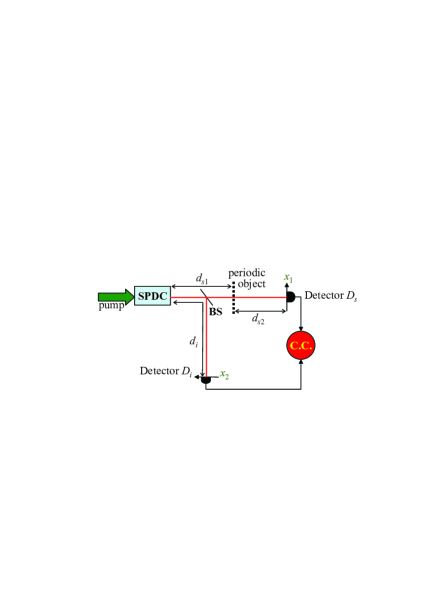
Figure 1: (color online) Setup to show the Talbot effect in quantum imaging using SPDC photons. BS, beamsplitter; C.C., coincidence counter.

Following the treatment in Goodman ; Rubin ; Wen , we evaluate the Green’s functions $g_{1}(\vec{\alpha}_{1},\omega_{s};\vec{\rho}_{1},d_{s})$ and $g_{2}(\vec{\alpha}_{2},\omega_{i};\vec{\rho}_{2},d_{i})$ in the paraxial approximation with an object described by the transparency function $A_{o}(\vec{\rho}_{o})$, and obtain

$$g_{1}(\vec{\alpha}_{1},\omega_{s};\vec{\rho}_{1},d_{s}) = -\frac{i\omega_{s}}{2\pi cd_{s2}}e^{i\frac{\omega_{s}}{c}d_{s}}e^{i\frac{\omega_{s}}{2cd_{s2}}\rho^{2}_{1}}e^{-i\frac{cd_{s1}}{2\omega_{s}}\alpha^{2}_{1}}$$

$$\times \int{d}^{2}\rho_{o}A_{o}(\vec{\rho}_{o})e^{i\frac{\omega_{s}\rho^{2}_{o}}{2cd_{s2}}}e^{i\vec{\rho}_{o}\cdot\left(\vec{\alpha}_{1}-\frac{\omega_{s}\vec{\rho}_{1}}{cd_{s2}}\right)},$$

$$\ g_{2}(\vec{\alpha}_{2},\omega_{i};\vec{\rho}_{2},d_{i}) = e^{i\frac{\omega_{i}}{c}d_{i}}e^{-i\frac{cd_{i}}{2\omega_{i}}\alpha^{2}_{2}}e^{i\vec{\alpha}_{2}\cdot\vec{\rho}_{2}},$$ (6)

where $d_{s}=d_{s1}+d_{s2}$ and $A_{o}(\vec{\rho}_{o})$ is the aperture function of the object. From Eqs. (3) and (5), and with the assumption that $\omega_{j}=\Omega_{j}+\nu_{j}$, where $|\nu_{j}|\ll\Omega_{j}$ and $\Omega_{s}+\Omega_{i}=\omega_{p}$, the temporal (longitudinal) and transverse terms can be factored out so the two-photon amplitude in Eq. (2) becomes

$$\Psi(\vec{r}_{1},t_{1};\vec{r}_{2},t_{2})=e^{i(\Omega_{s}\tau_{1}+\Omega_{i}\tau_{2})}\psi(\vec{\rho}_{1},\tau_{1};\vec{\rho}_{2},\tau_{2}),$$ (7)

where $\tau_{1}=t_{1}-d_{s}/c$, $\tau_{2}=t_{2}-d_{i}/c$, and

$$\psi(\vec{\rho}_{1},\tau_{1};\vec{\rho}_{2},\tau_{2}) = \int{d}\nu_{s}\int{d}\nu_{i}\delta(\nu_{s}+\nu_{i})e^{i(\nu_{s}\tau_{1}+\nu_{i}\tau_{2})}$$ (8)

$$\times f_{1}(\Omega_{s}+\nu_{s})f_{2}(\Omega_{i}+\nu_{i})B(\vec{\rho}_{1},\vec{\rho}_{2}).$$

The transverse part $B(\vec{\rho}_{1},\vec{\rho}_{2})$ takes the form

$$B(\vec{\rho}_{1},\vec{\rho}_{2}) = B_{0}\int{d}^{2}\rho_{o}A_{o}(\vec{\rho}_{o})e^{i\frac{\omega_{s}}{2cd_{s2}}\rho^{2}_{o}}e^{-i\frac{\omega_{s}}{cd_{s2}}\vec{\rho}_{o}\cdot\vec{\rho}_{1}}$$ (9)

$$\times \int{d}^{2}\alpha_{1}e^{-i\frac{c}{2}\alpha^{2}_{1}\left(\frac{d_{s1}}{\omega_{s}}+\frac{d_{i}}{\omega_{i}}\right)}e^{i\vec{\alpha}_{1}\cdot(\vec{\rho}_{o}-\vec{\rho}_{2})},$$

where we have collected all the slowly varying terms into the constant $B_{0}$. Completing the integration on the transverse mode $\vec{\alpha}_{1}$ in Eq. (9) gives

$$B(\vec{\rho}_{1},\vec{\rho}_{2}) = B_{0}\int{d}^{2}\rho_{o}A_{o}(\vec{\rho}_{o})$$ (10)

$$\times \textrm{exp}\left(-i\frac{\omega_{s}}{c}\vec{\rho}_{o}\cdot\left(\frac{\vec{\rho}_{1}}{d_{s2}}+\frac{\vec{\rho}_{2}}{d_{s1}+\frac{\omega_{s}}{\omega_{i}}d_{i}}\right)\right)$$

$$\times \textrm{exp}\left(i\frac{\omega_{s}}{2c}\rho^{2}_{o}\left(\frac{1}{d_{s2}}+\frac{1}{d_{s1}+\frac{\omega_{s}}{\omega_{i}}d_{i}}\right)\right).$$

Here again all the irrelevant constants have been absorbed into $B_{0}$.

For simplicity, our discussion will be restricted to one-dimensional objects, but extension of the analysis to two-dimensional objects is straightforward. The transmission function for a general one-dimensional periodic object can be expanded as a Fourier series

$$A_{o}(x)=\sum^{\infty}_{n=-\infty}c_{n}e^{-i\frac{2\pi{n}x}{a}},$$ (11)

where $a$ is the spatial period along the transverse $x$ direction and $c_{n}$ is the coefficient of the $n$th harmonic. We shall not specify the form of $c_{n}$ at this point, so any type of periodic object can be assumed for the present analysis. By substituting Eq. (11) into Eq. (10) and working in Cartesian coordinates, the transverse part of the two-photon amplitude in Eq. (10) can be written as

$$B(x_{1},x_{2}) = B_{0}\sum^{\infty}_{n=-\infty}c_{n}\textrm{exp}\left(-i\frac{\frac{n^{2}\pi}{a^{2}}\lambda_{s}}{\frac{1}{d_{s2}}+\frac{1}{d_{s1}+\frac{\lambda_{i}}{\lambda_{s}}d_{i}}}\right)$$ (12)

$$\times \textrm{exp}\left(i\frac{\frac{2\pi n}{a}\left(\frac{x_{1}}{d_{s2}}+\frac{x_{2}}{d_{s1}+\frac{\lambda_{i}}{\lambda_{s}}d_{i}}\right)}{\frac{1}{d_{s2}}+\frac{1}{d_{s1}+\frac{\lambda_{i}}{\lambda_{s}}d_{i}}}\right).$$

The exponential term in Eq. (12) is of basic importance to self-imaging, and will be called the “localization” term, since it describes the phase changes of the diffraction orders along the directions of propagation. It is known that self-imaging occurs in planes where the transmitted object light amplitudes are repeated, that is, when all diffraction orders are in phase and interfere constructively. From Eq. (12) we see that this can occur at certain distances when the first term equals $1$ for all $n$, that is,

$$\frac{1}{\lambda_{s}d_{s2}}+\frac{1}{\lambda_{s}d_{s1}+\lambda_{i}d_{i}}=\frac{1}{2ma^{2}},$$ (13)

where $m$ is an integer referred to as the self-imaging number. Defining $z_{s\textrm{\tiny}{T}}=2a^{2}/\lambda_{s}$, we can rewrite Eq. (13) as

$$\frac{1}{d_{s2}}+\frac{1}{d_{s1}+\frac{\lambda_{i}}{\lambda_{s}}d_{i}}=\frac{1}{mz_{s\textrm{\tiny}{T}}},$$ (14)

Comparing this with the well-known Gaussian thin lens equation, we can consider the self-imaging to be a counterpart phenomenon in which a sequence of lenses of focal length $z_{s\textrm{\tiny}{T}}$ is situated in the plane of the periodic object and produces images of the source. The distance $z_{s\textrm{\tiny}{T}}$ may be regarded as the Talbot length for second-order correlation quantum imaging.

We note that the factor $2$ in Eq. (13) is inconsequential, and so may be omitted. Thus in the cases when $m$ is an odd integer, there will be self-images with a lateral shift of half a period relative to the object, due to the $\pi$ phase shift of odd-number diffraction orders relative to the zero and even-number orders.

As mentioned in the previous section, in the self-image planes Eq. (12) reduces to

$$B(x_{1},x_{2})=B_{0}\sum^{\infty}_{n=-\infty}c_{n}e^{\left[i\frac{2\pi{n}}{a}\frac{\left(d_{s1}+\frac{\lambda_{i}}{\lambda_{s}}d_{i}\right)x_{1}+d_{s2}x_{2}}{d_{s1}+d_{s2}+\frac{\lambda_{i}}{\lambda_{s}}d_{i}}\right]},$$ (15)

which carries information about the lateral magnification $M$ of the imaging patterns arising as a result of the nonlocal correlation between entangled photons.

In a typical quantum imaging experiment, if the positions of the object and lens are specified, the lens equation immediately tells us the relationships between the image, object, and lens. This leads to the intuitive Klyshko interpretation of two-photon geometrical optics Klyshko , in which one of the photons is created at the detector placed in the same arm as the object, propagates back to the source where it becomes the second photon, which then propagates forward in time to the other detector. However, this picture may not be directly applicable to the second-order Talbot effect, because here, in principle, both detectors can be regarded as the source, and there are many complex cases with different possible magnifications. Nevertheless, there are two simple cases in which the Klyshko picture may be directly used to interpret the imaging process, that is, when either one of the detectors is fixed at its origin. This corresponds to either $x_{1}=0$ or $x_{2}=0$ in Eq. (15), in which case the images will be magnified by a factor of $1+\frac{d_{s1}+\lambda_{i}/\lambda_{s}d_{i}}{d_{s2}}$ or $1+\frac{d_{s2}}{d_{s1}+\lambda_{i}/\lambda_{s}d_{i}}$, respectively. Indeed, since both detectors could be visualized as point sources, two sets of self-images would be observable in coincidence measurements. The magnification for the images in such a case is not easy to describe since it depends on the detection scheme.

Before proceeding to the next section, we should check whether the Talbot effect could be observed with a single detector, so we should analyse the photon statistics in detector $D_{s}$ of Fig. 1. The single-photon count rate is defined as

$$R_{s}=\frac{1}{T}\int^{T}_{0}dt_{1}\sum_{\vec{k}_{i}}|\langle 0|a(\vec{k}_{i})E^{(+)}_{1}(\vec{r}_{1},t_{1})|\psi\rangle|^{2}.$$ (16)

Assuming there are infinite transverse modes in the SPDC process, with the use of Eqs. (3), (5), and (II.1) we find that in the transverse plane the single-photon counts is proportional to $\int{d}^{2}\rho_{o}|A_{o}(\vec{\rho}_{o})|^{2}$, so there is no diffraction image if only one detector is used.

II.2 Talbot effect in quantum lithography

In the proof-of-principle quantum lithography experiment of Boto , a factor of two over the classical diffraction limit was demonstrated by utilizing the entangled nature of a two-photon state. In this section we will extend our analysis to a quantum lithography experimental setup and see whether there is any difference in the Talbot self-imaging effect. In the scheme of Fig. 2, the periodic object is placed immediately behind the SPDC source, and we assume that the degenerate signal and idler photons ($\lambda_{s}=\lambda_{i}$) are detected by two single-photon detectors $D_{s}$ and $D_{i}$, or a two-photon detector without the beamsplitter. The distance between the object and the detectors is $d_{0}$. Following Goodman ; Rubin ; Wen , it is straightforward to show that the Green’s function for the signal ($j=1$) and idler ($j=2$) photons now takes the form of

$$g_{j}(\vec{\alpha}_{j},\omega;\vec{\rho}_{j},d) = -i\frac{e^{i\frac{\omega{d}}{c}}}{\lambda{d}}e^{i\frac{\omega\rho_{j}^{2}}{2cd}}\int{d}^{2}\rho_{o}A_{o}(\vec{\rho}_{o})e^{i\frac{\omega\rho^{2}_{o}}{2cd}}$$ (17)

$$\times e^{i\vec{\rho}_{o}\cdot(\vec{\alpha}_{j}-\frac{\omega\vec{\rho}_{j}}{cd})}.$$

By applying the same procedure in Sec. II A, the transverse part of the two-photon amplitude (8) now becomes

$$B(\vec{\rho}_{1},\vec{\rho}_{2})=B_{0}\int{d}^{2}\rho_{o}A^{2}_{o}(\vec{\rho}_{o})e^{i\frac{\omega\rho^{2}_{o}}{cd}}e^{-i\frac{\omega\vec{\rho}_{o}\cdot(\vec{\rho}_{1}+\vec{\rho}_{2})}{cd}}.$$ (18)

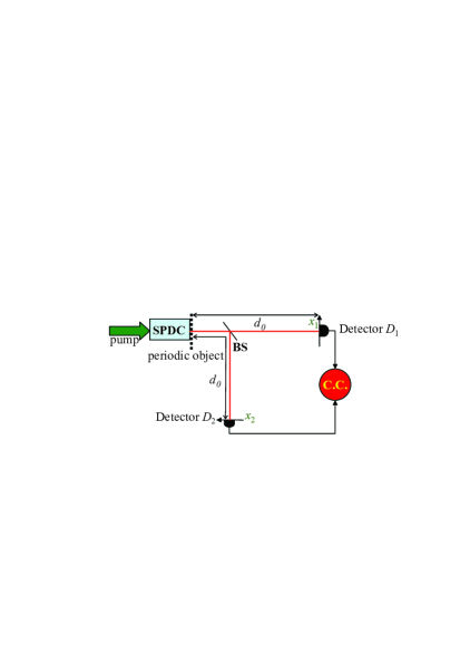
Figure 2: (color online) Scheme to demonstrate the Talbot effect using degenerate SPDC photons in the quantum lithography configuration. BS, beamsplitter; C.C., coincidence counter.

For simplicity, we still consider the one-dimensional periodic object given in Eq. (11). Plugging Eq. (11) into (18), we obtain

$$B(x_{1},x_{2})=B_{0}\sum^{\infty}_{n=-\infty}c^{2}_{n}e^{-i2\pi\frac{{n}^{2}}{a^{2}}\lambda d_{0}}e^{i\frac{2\pi{n}}{a}(x_{1}+x_{2})}.$$ (19)

As in our previous discussion, the condition for revival patterns of the periodic structure to occur is that the diffraction orders have equal phases when the distances $d_{0}$ satisfies

$$d_{0}=\frac{ma^{2}}{\lambda}=mz_{s\textrm{\tiny}{T}},$$ (20)

and Eq. (19) then reduces to

$$B(x_{1},x_{2})=B_{0}\sum^{\infty}_{n=-\infty}c^{2}_{n}e^{i\frac{2\pi{n}}{a}(x_{1}+x_{2})}.$$ (21)

This intensity-intensity correlation distribution is almost the same as that at the exit surface of the object. Similarly, as in the previous case, the self-imaging planes can be obtained by setting either detector at the origin. If the factor $m$ in Eq. (20) is an odd integer, the self-replicated diffraction pattern is also laterally displaced by half a period with respect to the original object.

We notice a number of interesting points from Eqs. (20) and (21). First, for a source of the same wavelength, $z_{s\textrm{\tiny}{T}}$ is only half of the classical first-order Talbot length $z_{\textrm{\tiny}{T}}$, but there is no magnification in the image. Secondly, for collinear degenerate SPDC as considered here, both entangled photons pass through the same spatial point in the object, so the Fourier coefficients $c_{n}$ become $c^{2}_{n}$. Thirdly, if a detector capable of resolving two photons were employed, an enhancement factor of $2$ in the self-images would be obtained compared with the classical first-order case.

II.3 Numerical Examples and Discussion

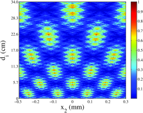
Figure 3: (color online) Second-order Talbot imaging carpet obtained by scanning the idler detector $D_{i}$ through $d_{i}=$ 0 – 34 cm along the longitudinal $z$ direction and through $x_{2}=-$ 0.3 – 0.3 mm in the transverse $x$ direction while keeping the signal detector $D_{s}$ fixed at position $d_{s2}=20$ cm and $x_{1}=0$, and $d_{s1}=11$ cm. The color bar denotes the transverse value of the two-photon correlation function.

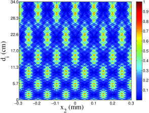
(a)  Second-order Talbot imaging carpet

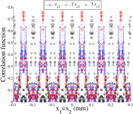
(b)  Second-order Talbot image

Figure 4: (color online) (a) Second-order Talbot imaging carpet obtained by moving both detectors synchronously along the transverse $x$ direction ($x_{1}=x_{2}=-$ 0.3 – 0.3 mm) and scanning the idler detector $D_{i}$ through $d_{i}=$ 0 – 34 cm along the $z$ direction while keeping the signal detector $D_{s}$ fixed at position $d_{s2}=20$ cm, with $d_{s1}=11$ cm. The color bar denotes the value of the transverse two-photon correlation function. (b) Second-order Talbot image obtained as in (a), but with $D_{i}$ at positions $d_{i}=z_{s\textrm{\tiny}{T}}$ (blue triangles), $d_{i}=2z_{s\textrm{\tiny}{T}}$ (red circles) and $d_{i}=5z_{s\textrm{\tiny}{T}}$ (black squares).

For convenience, we assume that both idler and signal photons are generated by SPDC at the wavelength $\lambda_{s}=\lambda_{i}=\lambda=883.2$ nm when light from a $441.6$ nm pump laser beam is incident on a nonlinear crystal, and the periodic object is a one dimensional rectangular grating $a=0.1$ mm. In the quantum imaging scheme, the main result of the second-order Talbot effect is represented by Eq. (12). Figure 3 shows the numerically computed second-order correlation pattern obtained by scanning the idler detector $D_{i}$ along the longitudinal $z$ and transverse $x$ directions while keeping the signal detector ($D_{s}$) fixed at position $d_{s2}$ and $x_{1}=0$, the distance $d_{s1}$ from the crystal to the periodic object also being fixed. We see that a typical Talbot “carpet” pattern is produced. In the same way, Fig. 4 (a) shows the second-order Talbot imaging carpet obtained when both detectors are moved synchronously along the transverse $x$ plane, with the signal detector $D_{s}$ fixed at position $d_{s2}=20$ cm, and the idler detector $D_{i}$ scanned along the longitudinal $z$ direction. The transverse profile of the “carpet” is given by the second-order Talbot image of Fig. 4 (b),where the self-image is obtained by moving both detectors synchronously in the $x$ direction, keeping $d_{s2}$ fixed, and the longitudinal positions of $D_{i}$ at $d_{i}=z_{s\textrm{\tiny}{T}}$ (blue triangles), $d_{i}=2z_{s\textrm{\tiny}{T}}$ (red circles), and $d_{i}=5z_{s\textrm{\tiny}{T}}$ (black squares). It is found that the second-order Talbot image produced by scanning only one detector is magnified, while that obtained by moving both detectors synchronously is the same size as the original object. It is interesting to note that the latter case holds even if the detectors are not at the same distance from the light source.

There are also some interesting features that may be observed from Eq. (19) in the quantum lithography case. The second-order Talbot length $z_{s\textrm{\tiny}{T}}=a^{2}/\lambda$ is only half the classical Talbot length $z_{\textrm{\tiny}{T}}=2a^{2}/\lambda$. Figure 5 shows the second-order interference pattern obtained by scanning both detectors along the $z$ direction in the region of $d_{0}=$ 0 – 5.7 cm while keeping the transverse position of one detector ($D_{s}$ or $D_{i}$) fixed at $x_{1}=0$ (or $x_{2}=0$), and scanning the other detector in the transverse direction. When both detectors are moved together along the transverse direction, we find that the period of the grating is halved, that is, the longitudinal resolution is enhanced by a factor of two. Moreover, when both detectors are displaced simultaneously in the same manner along the $x$ and $z$ directions, then not only is the longitudinal resolution increased but also the spatial resolution is improved by a factor of two, as shown in Fig. 6.

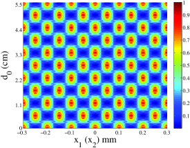
Figure 5: (color online) Second-order Talbot lithography carpet obtained by scanning both detectors $D_{i}$ and $D_{s}$ along the $z$ direction from $d_{0}=$ 0 – 5.7 cm with the transverse position of one detector fixed at $x_{1}(x_{2})=0$, and the other detector scanned in the transverse $x_{2}(x_{1})$ direction. The color bar denotes the value of the transverse two-photon correlation function.

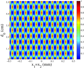
Figure 6: (color online) Second-order Talbot lithography carpet obtained by moving both detectors simultaneously in the same manner along the transverse $x$ and longitudinal $z$ directions. The transverse scanning range is $x_{1}=x_{2}=-$ 0.3 – 0.3 mm. The color bar denotes the value of the transverse two-photon correlation function.

In the above derivations we have implicitly assumed normal incidence of the illuminating fields to the object plane. It is possible to generalize our analysis to the case of non-normal incidence. A lateral displacement of the SPDC source from the optical axis would introduce a displacement of the observed second-order self-images proportional to the observation distance and incident angle Patorski . The same would be true for a nonparallel illumination beam. Moreover, the analysis throughout the paper is based on a plane-wave input beam, but it is possible to take into account the Gaussian profile of the pump.

It should be emphasized that the results obtained in Sections II A and B are valid when the parabolic approximation is satisfied for all diffraction orders. This implies that all diffraction orders are simultaneously co-phasial in the self-imaging planes. In classical wave optics, this problem was addressed, for example, by Sciammarella and Davis Scimmarella and Chang Chang . By setting a tolerance on the maximum allowable optical path difference introduced by the third term in the binomial expansion of $\sqrt{1+(\rho/z)^{2}}$, one can determine the maximum number $m$ of the self-images formed by a specified diffraction order $n$ of the object. At larger observation distances, due to gradual violation of the paraxial approximation by higher diffraction orders, one can no longer speak of “self-imaging” in the strict sense. Experimentally, the images would become more and more blurred.

Before concluding this section, we should remark that the Talbot self-imaging effect with entangled photon pairs studied here can be generalized to multiphoton entangled states Wen ; Wen2 . Although the realization of entangled multiphoton sources is experimentally challenging, the inherent physics would be of great richness and well worth studying.

III Summary

In summary, we have theoretically studied quantum ghost imaging with a periodic structure as the object, illuminated by entangled photon pairs generated from SPDC with a plane-wave incident pump. It is shown that a second-order Talbot effect (self-imaging effect) in both the quantum imaging and lithography configurations may be observed, without the need of any focussing lens. The self-images observed in the two-photon coincidence counts are nonlocal, and there is no imaging in the single-photon counts. In the quantum imaging setup, the Klyshko picture of two-photon geometric optics may be applied to interpret the imaging process under certain conditions. In the quantum lithographic configuration, we show that the Talbot length is half of that in the classical first-order case.

We also notice that the quadratic phases shown in the origin of the Talbot effect have played an important role in revivals and fractional revivals Leichtle , curlicues Berry , quantum carpets Marzoli , and Gaussian sums Mack . It is to be hoped that many other interesting second-order phenomena based on entangled photons may result from our above analysis.

IV Acknowledgments

We thank Sai-Jun Wu and Morton H. Rubin for helpful discussions. This work was supported by the National Natural Science Foundation of China (Grant No 10674174) and the National Program for Basic Research in China (Grant 2006CB921107). J.W. and M.X. acknowledge partial support from the National Science Foundation of the U.S.A.

References

- (1) H. F. Talbot, Philos. Mag. 9, 401 (1836).
- (2) L. Rayleigh, Philos. Mag. 11, 196 (1881).
- (3) H. Weisel, Ann. Phys. Lpz. 33, 995 (1910).
- (4) M. Wolfke, Ann. Phys. Lpz. 40, 194 (1913).
- (5) J. T. Winthrop and C. R. Worthington, J. Opt. Soc. Am. 55, 373-381 (1965)
- (6) K. Patorski, in Progress in Optics 27, pp. 1-108, edited by E. Wolf (North-Holland, Amsterdam, 1989).
- (7) J. M. Cowley and A. F. Moodie, Proc. Phys. Soc. B 70, 486 (1957); 70, 497 (1957); 70, 505 (1957); J. M. Cowley, Diffraction Physics (North-Holland, Amsterdam, 1995).
- (8) M. S. Chapman, C. R. Ekstrom, T. D. Hammond, J. Schmiedmayer, B. E. Tannian, S. Wehinger, and D. E. Pritchard, Phys. Rev. A 51, R14 (1995).
- (9) S. Wu, E. Su, and M. Prentiss, Phys. Rev. Lett. 99, 173201 (2007).
- (10) L. Deng, E. W. Hagley, J. Denschlag, J. E. Simsarian, M. Edwards, C. W. Clark, K. Helmerson, S. L. Rolston, and W. D. Phillips, Phys. Rev. Lett. 83, 5407 (1999).
- (11) Ke Li, L. Deng, E.W. Hagley, M. G. Payne, and M. S. Zhan, Phys. Rev. Lett. 101, 250401 (2008).
- (12) B. Brezger, L. Hackemüller, S. Uttenthaler, J. Petschinka, M. Arndt, and A. Zeilinger, Phys. Rev. Lett. 88, 100404 (2002).
- (13) R. Iwanow, D. A. May-Arrioja, D. N. Christodoulides, G. I. Stegeman, Y. Min, and W. Sohler, Phys. Rev. Lett. 95, 053902 (2005).
- (14) T. Weitkamp, B. Nöhammer, A. Diaz, and C. David, Appl. Phys. Lett. 86, 54101-54103 (2005).
- (15) T. B. Pittman, Y.-H. Shih, D. V. Strekalov, and A. V. Sergienko, Phys. Rev. A 52, R3429 (1995).
- (16) D. V. Strekalov, A. V. Sergienko, D. N. Klyshko, and Y.-H. Shih, Phys. Rev. Lett. 74, 3600 (1995).
- (17) I. Vidal, S. B. Cavalcanti, E. J. S. Fonseca, and J. M. Hickmann, Phys. Rev. A 78, 033829 (2008).
- (18) D. N. Klyshko, Phys. Lett. A 128, 1337 (1988); Sov. Phys. Usp. 31, 74 (1988).
- (19) J. W. Goodman, Introduction to Fourier Optics (McGraw-Hill, New York, 1968).
- (20) M. H. Rubin, Phys. Rev. A 54, 5349 (1996).
- (21) J.-M. Wen, P. Xu, M. H. Rubin, and Y.-H. Shih, Phys. Rev. A 76, 023828 (2007).
- (22) A. N. Boto, P. Kok, D. S. Abrams, S. L. Braunstein, C. P. Williams, and J. P. Dowling, Phys. Rev. Lett. 85, 2733 (2000)
- (23) C. A. Scimmarella and D. Davis, Exp. Mech. 8, 459 (1968).
- (24) B. J. Chang, Ph.D. Thesis, University of Michigan (1974).
- (25) J.-M. Wen and M. H. Rubin, Phys. Rev. A 79, 025802 (2009).
- (26) C. Leichtle, I. S. Averbukh, and W. P. Schleich, Phys. Rev. Lett. 77, 3999 (1996).
- (27) M. V. Berry and J. Goldberg, Nonlinearity 1, 1 (1988); M. V. Berry and S. Klein, J. Mod. Opt. 43, 2139 (1996).
- (28) M. V. Berry, I. Marzoli, and W. P. Schleich, Phys. World 14, 39 (2001); O. Friesch, I. Marzoli, and W. P. Schleich, New J. Phys. 2, 4 (2000).
- (29) H. Mack, M. Bienert, F. Haug, M. Freyberger, and W. P. Schleich, Phys. Stat. Sol. (b) 233, 408 (2002).