Telling cause from effect
based on high-dimensional observations

Abstract

We describe a method for inferring linear causal relations among multi-dimensional variables. The idea is to use an asymmetry between the distributions of cause and effect that occurs if both the covariance matrix of the cause and the structure matrix mapping cause to the effect are independently chosen. The method works for both stochastic and deterministic causal relations, provided that the dimensionality is sufficiently high (in some experiments, $5$ was enough). It is applicable to Gaussian as well as non-Gaussian data.

1 Motivation

Inferring the causal relations that have generated statistical dependencies among a set of observed random variables is challenging if no controlled randomized studies can be made. Here, causal relations are represented as arrows connecting the variables, and the structure to be inferred is a directed acyclic graph (DAG) [1, 2]. The constraint-based approach to causal discovery, one of the best known methods, selects directed acyclic graphs that satisfy both the causal Markov condition and faithfulness: One accepts only those causal hypotheses that explain the observed dependencies and demand that all the observed independencies are imposed by the structure, i.e., common to all distributions that can be generated by the respective causal DAG. However, the methods are fundamentally unable to distinguish between DAGs that induce the same set of dependencies (Markov-equivalent graphs). Moreover, causal faithfulness is known to be violated if some of the causal relations are deterministic [3]. Solving these problem requires reasonable prior assumptions, either implicitly or explicitly as priors on conditional probabilities, as in Bayesian settings [4]. However, the fact that deterministic dependencies exist in real-world settings shows that priors that are densities on the parameters of the Bayesian networks, as it is usually assumed, are problematic, and the construction of good priors becomes difficult.

Recently, several methods have been proposed that are able to distinguish between Markov-equivalent DAGs. Linear causal relations among non-Gaussian random variables can be inferred via independent-component-analysis (ICA) methods [6, 7]. The method of [8] is able to infer causal directions among real-valued variables if every effect is a (possibly non-linear) function of its causes up to an additive noise term that is independent of the causes. The work of [9] augmented these models by applying a non-linear function after adding the noise term. If the noise term vanishes or if all of the variables are Gaussian and the relation is linear, all these methods fail. Moreover, if the data are high-dimensional, the non-linear regression involved in the methods becomes hard to estimate.

Here we present a method that also works for these cases provided that the variables are multi-dimensional with sufficiently anisotropic covariance matrices. The underlying idea is that the causal hypothesis $X\rightarrow Y$ is only acceptable if the shortest description of the joint distribution $P(X,Y)$ is given by separate descriptions of the input distribution $P(X)$ and the conditional distribution $P(Y|X)$ [10], expressing the fact that they represent independent mechanisms of nature. [11] shows toy examples where such an independent choice often leads to joint distributions where $P(Y)$ and $P(X|Y)$ satisfy non-generic relations indicating that $Y\rightarrow X$ is wrong. Here we develop this idea for the case of multi-dimensional variables $X$ and $Y$ with a linear causal relation.

We start with a motivating example. Assume that $X$ is a multivariate Gaussian variable with values in ${\mathbb{R}}^{n}$ and the isotropic covariance matrix $C_{XX}={\bf I}$. Let $Y$ be another ${\mathbb{R}}^{n}$-valued variable that is deterministically influenced by $X$ via the linear relation $Y=AX$ for some $n\times n$-matrix $A$. This induces the covariance matrix

$$C_{YY}=AC_{XX}A^{T}=AA^{T}.$$

The converse causal hypothesis $Y\rightarrow X$ becomes unlikely because $P(Y)$ (which is determined by the covariance matrix $AA^{T}$) and $P(X|Y)$ (which is given by $X=A^{-1}Y$ with probability $1$) are related in a suspicious way, since the same matrix $A$ appears in both descriptions. This untypical relationship between $P(Y)$ and $P(X|Y)$ can also be considered from the point of view of symmetries: consider the set of covariance matrices $UC_{YY}U^{T}$ with $U\in O(n)$, where $O(n)$ denotes the orthogonal group. Among them, $C_{YY}$ is special because it is the only one that is transformed into the isotropic covariance matrix $C_{XX}$. More generally speaking, in light of the fact of how anisotropic the matrices

$$\tilde{C}_{XX}:=A^{-1}UC_{YY}U^{T}A^{-T}$$

are for generic $U$, the hypothetical effect variable is surprisingly isotropic for $U={\bf I}$ (here we have used the short notation $A^{-T}:=(A^{-1})^{T}$). We will show below that this remains true with high probability (in high dimensions) if we start with an arbitrary covariance matrix $C_{XX}$ and apply a random linear transformation $A$ chosen independently of $C_{XX}$.

To understand why independent choices of $C_{XX}$ and $A$ typically induce untypical relations between $A^{-1}$ and $C_{YY}$ we also discuss the simple case that $C_{XX}$ and $A$ are simultaneously diagonal with $c_{j}$ and $a_{j}$ as corresponding diagonal entries. Thus $C_{YY}$ is also diagonal and its diagonal entries (eigenvalues) are $a_{j}^{2}c_{j}$. We now assume that “nature has chosen” the values $c_{j}$ with $j=1,\dots,n$ independently from some distribution and $a_{j}$ from some other distribution. We can then interpret the values $c_{j}$ as instances of $n$-fold sampling of the random variable $c$ with expectation ${\mathbb{E}}(c)$ and the same for $a_{j}$. If we assume that $a$ and $c$ are independent, we have

$${\mathbb{E}}(a^{2}c)={\mathbb{E}}(a^{2}){\mathbb{E}}(c)\,.$$ (1)

Due to the law of large numbers, this equation will for large $n$ approximatively be satisfied by the empirical averages, i.e.,

$$\frac{1}{n}\sum_{j=1}^{n}a^{2}_{j}c_{j}\approx\left(\frac{1}{n}\sum_{j=1}^{n}a_{j}^{2}\right)\,\left(\frac{1}{n}\sum_{j=1}^{n}c_{j}\right)\,.$$ (2)

For the backward direction $Y\rightarrow X$ we observe that the diagonal entries $\tilde{c}_{j}=c_{j}a_{j}^{2}$ of $C_{YY}$ and the diagonal entries $\tilde{a}_{j}=a_{j}^{-1}$ of $\tilde{A}:=A^{-1}$ have not been chosen independently because

$${\mathbb{E}}(\tilde{a}^{2}\tilde{c})={\mathbb{E}}(c)\,,$$

whereas

$${\mathbb{E}}(\tilde{a}^{2}){\mathbb{E}}(\tilde{c}) = {\mathbb{E}}(a^{-2}){\mathbb{E}}(a^{2}c)={\mathbb{E}}(a^{-2}){\mathbb{E}}(a^{2}){\mathbb{E}}(c)>{\mathbb{E}}(c)\,.$$

The last inequality holds because the random variables $a^{2}$ and $a^{-2}$ are always negatively correlated (this follows easily from the Cauchy-Schwarz inequality ${\mathbb{E}}(a^{2}){\mathbb{E}}(a^{-2})\leq 1$) except for the trivial case when they are constant. We thus observe a systematic violation of (1) in the backward direction. The proof for non-diagonal matrices in Section 2 uses standard spectral theory, but is based upon the same idea.

The paper is structured as follows. In Section 2, we define an expression with traces on covariance matrices and show that typical linear models induce backward models for which this expression attains values that would be untypical for the forward direction. In Section 3 we describe an algorithm that is based upon this result and discuss experiments with simulated and real data. Section 4 proposes possible generalizations.

2 Identifiability results

Given a hypothetical causal model $Y=AX+E$ (where $X$ and $Y$ are $n$- and $m$-dimensional, respectively) we want to check whether the pair $(C_{XX},A)$ satisfies some relation that typical pairs $(UC_{XX}U^{T},A)$ only satisfy with low probability if $U\in O(n)$ is randomly chosen. To this end, we introduce the renormalized trace

$$\tau_{n}(.):={\tt tr}(.)/n$$

for dimension $n$ and compare the values

$$\tau_{m}(AC_{XX}A^{T})\quad\hbox{ and }\quad\tau_{n}(C_{XX})\tau_{m}(AA^{T})\,.$$ (3)

One shows easily that the expectation of both values coincide if $C_{XX}$ is randomly drawn from a distribution that is invariant under transformations

$$C_{XX}\mapsto UC_{XX}U^{T}.$$

This is because averaging the matrices $UC_{XX}U^{T}$ over all $U\in O(n)$ projects onto $\tau_{n}(C_{XX}){\bf I}$ since the average $UC_{XX}U^{T}$ commutes with all matrices and is therefore a multiple of the identity. For our purposes, it is decisive that the typical case is close to this average, i.e., the two expressions in (3) almost coincide. To show this, we need the following result [13]:

Lemma 1 (Lévy’s Lemma)

Let $g:S_{n}\rightarrow{\mathbb{R}}$ be a Lipschitz continuous function on the $n$-dimensional sphere with

$$L:=\max_{\gamma\neq\gamma^{\prime}}\frac{|g(\gamma)-g(\gamma^{\prime})|}{\|\gamma-\gamma^{\prime}\|}\,.$$

If a point $\gamma$ on $S_{n}$ is randomly chosen according to an $O(n)$-invariant prior, it satisfies

$$|g(\gamma)-\bar{g}|\leq\epsilon$$

with probability at least $1-\exp(-\kappa(n-1)\epsilon^{2}/L^{2})$ for some constant $\kappa$, where $\bar{g}$ can be interpreted as the median or the average of $g(\gamma)$.

Given the above Lemma, we can prove the following Theorem:

Theorem 1 (traces are typically multiplicative)

Let $C$ be a symmetric, positive definite $n\times n$-matrix and $A$ an arbitrary $m\times n$-matrix. Let $U$ be randomly chosen from $O(n)$ according to the unique $O(n)$-invariant distribution (i.e. the Haar measure). Introducing the operator norm

$$\|B\|:=\max_{\|x\|=1}\|Bx\|,$$

we have

$$|\tau_{m}(AUCU^{T}A^{T})-\tau_{n}(C)\tau_{m}(AA^{T})|\leq 2\epsilon\|C\|\|AA^{T}\|$$

with probability at least $q:=1-\exp(-\kappa(n-1)\epsilon^{2})$ for some constant $\kappa$ (independent of $C,A,n,m,\epsilon$).

Proof: for an arbitrary orthonormal system $(\psi_{j})_{j=1,\dots,m}$ we have

$$\tau_{m}(AUCU^{T}A^{T})=\frac{1}{m}\sum_{j=1}^{m}\langle\psi_{j},AUCU^{T}A^{T}\psi_{j}\rangle\,.$$

We define the unit vectors

$$\gamma_{j}:=U^{T}A^{T}\psi_{j}/\|A^{T}\psi_{j}\|.$$

Dropping the index $j$, we introduce the function

$$f(\gamma):=\langle\gamma,C\gamma\rangle\,.$$

For a randomly chosen $U\in O(n)$, $\gamma$ is a randomly chosen unit vector according to a uniform prior on the $n$-dimensional sphere $S_{n}$.

The average of $f$ is given by $\bar{f}=\tau_{n}(C)$. The Lipschitz constant is given by the operator norm of $C$, i.e., $L=2\|C\|\,.$ An arbitrarily chosen $j$ satisfies

$$|\langle\gamma_{j},C\gamma_{j}\rangle-\tau_{n}(C)|\leq 2\epsilon\|C\|$$

with probability $1-\exp(-\kappa(n-1)\epsilon^{2})$. This follows from Lemma 1 after replacing $\epsilon$ with $\epsilon L$. Hence

$$|\langle\psi_{j},AUCU^{T}A^{T}\psi_{j}\rangle-\tau_{n}(C)\langle\psi_{j},AA^{T}\psi_{j}\rangle|\leq 2\epsilon\|C\|\|AA^{T}\|\,.$$

Due to

$$\tau_{m}(AUCU^{T}A^{T})=\frac{1}{m}\sum_{j=1}^{m}\langle\psi_{j},AA^{T}\psi_{j}\rangle\langle\gamma_{j},C\gamma_{j}\rangle\,,$$

we thus have

$$|\tau_{m}(AUCU^{T}A^{T})-\tau_{m}(AA^{T})\tau_{n}(C)|\leq 2\epsilon\|C\|\|AA^{T}\|\,.$$

$\Box$

It is convenient to introduce

$$\Delta(C,A):=\log\tau_{m}(ACA^{T})-\log\tau_{n}(C)-\log\tau_{m}(AA^{T})$$

as a scale-invariant measure for the strength of the violation of the equality of the expressions (3).

We now restrict the attention to two special cases where we can show that $\Delta$ is non-zero for the backward direction. First, we restrict the attention to deterministic models

$$Y=AX$$

and the case that $m\geq n$ where $A$ has rank $n$. This ensures that the backward model is also deterministic, i.e.,

$$X=A^{-1}Y\,,$$

with $(.)^{-1}$ denoting the pseudo inverse.

The following theorem shows that $\Delta(C_{XX},A)=0$ implies $\Delta(C_{YY},A^{-1})<0$:

Theorem 2 (systematic violation of trace multiplicativity)

Let $n$ and $m$ denote the dimensions of $X$ and $Y$, respectively. If $Y=AX$ and $X=A^{-1}Y$, the covariance matrices satisfy

$$\Delta(C_{XX},A)+\Delta(C_{YY},A^{-1})=-\log\left(1-{\tt Cov}(Z,1/Z)\right)+\log\frac{n}{m}\,,$$ (4)

where $Z$ is a real-valued random variable whose distribution is the empirical distribution of eigenvalues of $AA^{T}$, i.e., $\tau_{m}((AA^{T})^{k})={\mathbb{E}}(Z^{k})$ for all $k\in{\mathbb{N}}$.

Proof: We have

$$\frac{\tau_{n}(C)}{\tau_{m}(ACA^{T})\tau_{n}(A^{-1}A^{-T})}=\frac{1}{\tau_{m}(AA^{T})\tau_{n}(A^{-1}A^{-T})}\frac{\tau_{n}(C)\tau_{m}(A^{T}A)}{\tau_{m}(ACA^{T})}\,.$$ (5)

Using

$$\tau_{n}(A^{-1}A^{-T})=\tau_{n}(A^{-T}A^{-1})=\tau_{n}((AA^{T})^{-1})=\frac{m}{n}\tau_{m}((AA^{T})^{-1})$$

and taking the logarithm we obtain

$$\Delta(ACA^{T},A^{-1})=\log\frac{1}{{\mathbb{E}}(Z){\mathbb{E}}(1/Z)}+\log\frac{n}{m}-\Delta(C,A)\,.$$

Then the statement follows from

$${\tt Cov}(Z,1/Z)=1-{\mathbb{E}}(Z){\mathbb{E}}(1/Z)\,.$$

$\Box$

Note that the term $-\log\left(1-{\tt Cov}(Z,1/Z)\right)$ in eq. (4) will not converge to zero for dimension to infinity if the random matrices $A$ are drawn in a way that ensures that the distribution of $Z$ converges to some distribution on ${\mathbb{R}}$ with non-zero variance. Assuming this, $\Delta(C_{YY},A^{-1})$ tends to some negative value if $\Delta(C_{XX},A)$ tends to zero for $n=m\to\infty$.

We should, however, mention a problem that occurs for $m>n$ in the noise-less case discussed here: Since $C_{YY}$ has only rank $n$, we could equally well replace $A^{-1}$ with some other matrix $\hat{A}$ that coincides with $A^{-1}$ on all of the observed $y$-values. For those matrices $\hat{A}$, the value $\Delta$ can get closer to zero because the term $\log n/m$ expresses the fact that the image of $C_{YY}$ is orthogonal to the kernel of $A^{-1}$, which is already untypical for a generic model.

It turns out that the observed violation of the multiplicativity of traces can be interpreted in terms of relative entropy distances. To show this, we need the following result:

Lemma 2 (relative entropy in terms of determinants and traces)

Let $C$ be the covariance matrix of a centralized non-degenerate multi-variate Gaussian distribution $P_{C}$ in $n$ dimensions. Let the anisotropy of $C$ be defined by the relative entropy distance to the closest isotropic Gaussian

$$D(C):=\min_{Q\hbox{ isotropic }}D(P_{C}||Q)\,.$$

Then

$$D(C)=\frac{1}{2}\left(n\log\tau_{n}(C)-\log{\tt det}(C)\right)\,.$$ (6)

Proof: the relative entropy distance of two centralized Gaussians with covariance matrices $C,C_{0}$ in $n$ dimensions is given by

$$D(P_{C}||P_{C_{0}})=\frac{1}{2}\left(\log\Big{(}\frac{{\tt det}C_{0}}{{\tt det}C}\Big{)}+{\tt tr}(C_{0}^{-1}C)-n\right)\,.$$

Setting $C_{0}=\lambda{\bf I}$, the distance is minimized for $\lambda=\tau_{n}(C)$, which yields eq. (6). $\Box$

Straightforward computations show:

Theorem 3 (multiplicativity of traces and relative entropy)

Let $C$ and $A$ be $n\times n$-matrices with $C$ positive definite. Then

$$D(ACA^{T})=D(C)+D(AA^{T})+\Delta(C,A)\,.$$

Hence, for independently chosen $A$ and $C$, the anisotropy of the output covariance matrix $ACA^{T}$ is approximately given by the anisotropy of $C$ plus the anisotropy of $AA^{T}$, which is the anisotropy of the output that $A$ induces on an isotropic input. For the backward direction, the anisotropy is smaller than the typical value.

We now discuss an example with a stochastic relation between $X$ and $Y$. We first consider the general linear model

$$Y=AX+E\,,$$

where $A$ is an $n\times m$ matrix and $E$ is a noise term (statistically independent of $X$) with covariance matrix $C_{EE}$. We obtain

$$C_{YY}=AC_{XX}A^{T}+C_{EE}\,.$$

The corresponding backward model reads

$$X=\tilde{A}Y+\tilde{E}\,.$$

with

$$\tilde{A}:=C_{XY}C_{YY}^{-1}\,.$$

Now we focus on the special case where $A$ is an orthogonal transformation and $E$ is isotropic, i.e., $C_{EE}=\lambda{\bf I}$ with $\lambda>0$. We then obtain a case where $C_{YY}$ and $\tilde{A}$ are related in a way that makes $\Delta(C_{YY},\tilde{A})$ positive:

Lemma 3 (violation of multiplicativity of traces for a special noisy case)

Let $Y=AX+E$ with $A\in O(n)$ and the covariance matrix of $E$ be given by $C_{EE}=\lambda{\bf I}$. Then we have

$$\Delta(C_{YY},\tilde{A})>0\,.$$

Proof: We have

$$C_{YY}=ACA^{T}+\lambda{\bf I}\quad\hbox{ and }\quad C_{YX}=AC\,,$$

with $C:=C_{XX}$. Therefore,

$$\tilde{A}=CA^{T}(ACA^{T}+\lambda{\bf I})^{-1}=C(C+\lambda{\bf I})^{-1}A^{T}.$$

One checks easily that the orthogonal transformation $A$ is irrelevant for the traces and we thus have

$$\Delta(C_{YY},\tilde{A})=\log\frac{\tau(C^{2}(C+\lambda{\bf I})^{-1})}{\tau(C+\lambda{\bf I})\tau(C^{2}(C+\lambda{\bf I})^{-2})}=\log\frac{{\mathbb{E}}\left(Z^{2}/(Z+\lambda)\right)}{{\mathbb{E}}(Z+\lambda){\mathbb{E}}\left(Z^{2}/(Z+\lambda)^{2}\right)}\,,$$

where $Z$ is a random variable of which distribution reflects the distribution of eigenvalues of $C$. The function $z\mapsto z/(z+\lambda)$ is monotonously increasing for positive $\lambda$ and $z$ and thus also $z\mapsto z^{2}/(z+\lambda)^{2}$. Hence $Z+\lambda$ and $Z^{2}/(Z+\lambda)^{2}$ are positively correlated, i.e.,

$${\mathbb{E}}(Z^{2}/(Z+\lambda))={\mathbb{E}}((Z+\lambda)Z^{2}/(Z+\lambda)^{2})>{\mathbb{E}}(Z+\lambda){\mathbb{E}}\left(Z^{2}/(Z+\lambda)^{2}\right)\,,$$

for all distributions of $Z$ with non-zero variance. Hence the logarithm is positive and thus $\Delta(C_{YY},\tilde{A})>0$. $\Box$

Since the violation of the equality of the terms in (3) can be in both directions, we propose to prefer the causal direction for which $\Delta$ is closer to zero.

3 Inference algorithm and experiments

Motivated by the above theoretical results, we propose to infer the causal direction using Alg. 1.

Algorithm 1 Identifying linear causal relations via traces

1:  Input: $(x_{1},y_{1}),\ldots,(x_{k},y_{k})$

2:   Compute the estimators $C_{XX}$, $C_{XY}$, $C_{YX}$, $C_{YY}$

3:  Compute $A:=C_{YX}C_{XX}^{-1}$

4:  Compute $\tilde{A}:=C_{XY}C_{YY}^{-1}$

5:  if $|\log\tau_{m}(AC_{XX}A^{T})-\log\tau_{n}(C_{XX})-\log\tau_{m}(AA^{T})|>\epsilon+|\log\tau_{n}(\tilde{A}C_{YY}\tilde{A}^{T})-\log\tau_{m}(C_{YY})-\log\tau_{n}(\tilde{A}\tilde{A}^{T})|$ then

6:     write “$Y$ is the cause”

7:  else

8:     if $|\log\tau_{n}(\tilde{A}C_{YY}\tilde{A}^{T})-\log\tau_{m}(C_{YY})-\log\tau_{n}(\tilde{A}\tilde{A}^{T})|>\epsilon+|\log\tau_{m}(AC_{XX}A^{T})-\log\tau_{n}(C_{XX})-\log\tau_{m}(AA^{T})|$ then

9:        write “$X$ is the cause”

10:     else

11:        write “cause cannot be identified”

12:     end if

13:  end if

In light of the theoretical results, the following issues have to be clarified by experiments with simulated data:

1. Is the limit for dimension to infinity already justified for moderate dimensions?

2. Is the multiplicativity of traces sufficiently violated for noisy models?

Furthermore, the following issue has to be clarified by experiments with real data:

1. Is the behaviour of real causal structures qualitatively sufficiently close to our model with independent choices of $A$ and $C_{XX}$ according to a uniform prior?

For the simulated data, we have generated random models $Y=AX+E$ as follows: We independently draw each element of the $m\times n$ structure matrix $A$ from a standardized Gaussian distribution. This implies that the distribution of column vectors as well as the distribution of row vectors is isotropic. To generate a random covariance matrix $C_{XX}$, we similarly draw an $n\times n$ matrix $B$ and set $C_{XX}:=BB^{T}$. Due to the invariance of our decision rule with respect to the scaling of $A$ and $C_{XX}$, the structure matrix and the covariance can have the same scale without loss of generality. The covariance $C_{EE}$ of the noise is generated in the same way, although with an adjustable parameter $\sigma$ governing the scaling of the noise with respect to the signal: $\sigma=0$ yields the deterministic setting, while $\sigma=1$ equates the power of the noise to that of the signal.

First, we demonstrate the performance of the method in the close-to deterministic setting ($\sigma=0.05$) as a function of the dimensionality $n=m$ of the simulations, ranging from dimension 2 to 50. To show that the method is feasible even with a relatively small number of samples, we choose the number of samples $N$ to scale with the dimension as $N=2n$. (Note that we must have $N\geq\min(n,m)$ to obtain invertible estimates of the covariance matrices.) The resulting proportion of correct vs wrong decisions is given in Fig. 1a, with the corresponding values of $\Delta$ in Fig. 1b. As can be seen, even at as few as 5 dimensions and 10 samples, the method is able to reliably identify the direction of causality in these simulations.

a                        b                        c                        d

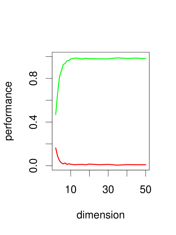
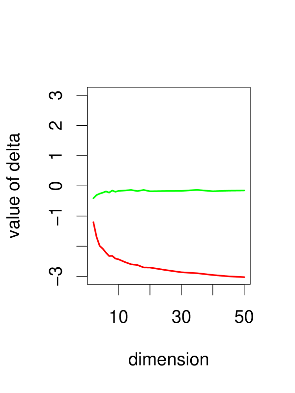
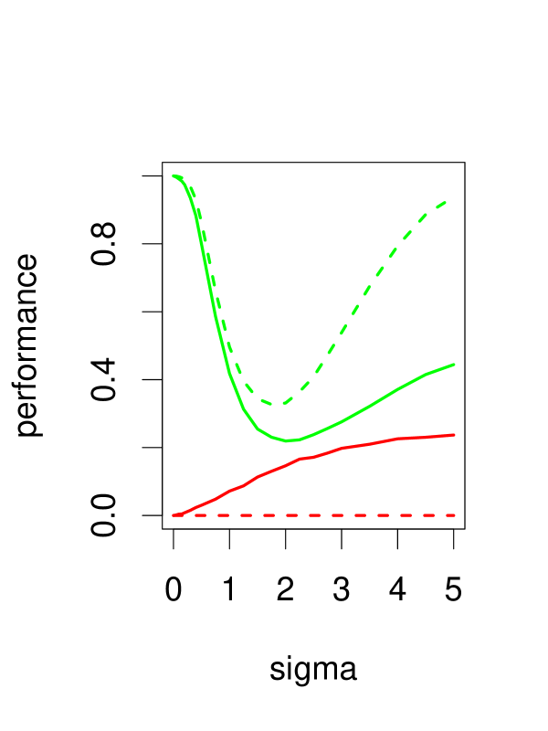
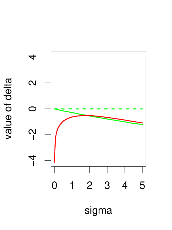
Figure 1: Simulation results. (a) Performance of the method as a function of the input dimensionality $n$, when the output dimensionality $m=n$ and the sample size is $N=2n$. The green curve denotes the fraction of simulations on which the true causal direction was selected, while the red curve gives the fraction of wrong answers. (b) Mean values of $\Delta$ corresponding to the true direction (green) vs the wrong direction (red). (c) Performance as a function of noise level $\sigma$, for dimensionality $n=m=10$ and sample size $N=1000$. To compare, the dashed lines give the performance based on the exact covariance matrices rather than based on the samples. (d) Mean values of $\Delta$ corresponding to the true direction (green) vs the wrong direction (red). See main text for discussion.

To illustrate the degree to which identifiability is hampered by noise, the solid line in Fig. 1c gives the performance of the method for a fixed dimension ($n=m=10$) and fixed sample size ($N=1000$) as a function of the noise level $\sigma$. As can be seen, the performance drops markedly as $\sigma$ is increased. As soon as there is significantly more noise than signal (say, $\sigma>2$), the number of samples is not sufficient to reliably estimate the required covariance matrices and hence the direction of causality. This is clear from looking at the much better performance of the method when based on the exact, true covariance matrices, given by the dashed lines. In Fig. 1d we show the corresponding values of $\Delta$, from which it is clear that the estimate based on the samples is quite biased for the forward direction.

As experiments with real data with known ground truth, we have chosen $16\times 16$ pixel images of handwritten digits [14]. As the linear map $A$ we have used both random local translation-invariant linear filters and also standard blurring of the images. (We added a small amount of noise to both original and processed images, to avoid problems with very close-to singular covariances.) See Fig. 2 for some example original and processed image pairs. The task is then: given a sample of pairs $(x_{1},y_{1})$ consisting of the picture $x_{j}$ and its processed counterpart $y_{j}$ infer which of the set of pictures $x$ or $y$ are the originals (‘causes’). By partitioning the image set by the digit class (0-9), and by testing a variety of random filters (and the standard blur), we obtained a number of test cases to run our algorithm on. Out of the total of 100 tested cases, the method was able to correctly identify the set of original images 94 times, with 4 unknowns (i.e. only two falsely classified cases).

These simulations and experiments are quite preliminary and mainly serve to illustrate the theory developed in the paper. They point out at least one important issue for future work: the construction of unbiased estimators for the trace values or the $\Delta$. The systematic deviation of the sample-based experiments from the covariance-matrix based experiments in Fig. 1c–d suggest that this could be a major improvement.

4 Outlook: generalizations of the method

In this section, we want to rephrase our theoretical results in a more abstract way to show the general structure. We have rejected the causal hypothesis $X\rightarrow Y$ if we observe that $\tau_{n}(AC_{XX}A^{T})$ attains values that are not typical among the set of transformed input covariance matrices $UC_{XX}U^{T}$. In principle, we could have any function $K$ that maps the output distribution $P(Y)$ to some value $K(P(Y))$. Moreover, we could have any group $G$ of transformations $g$ on the input variable $X$ that define transformed input distributions via

$$P_{g}(X)=P(g^{-1}X)\,.$$

Applying the conditional $P(Y|X)$ to $P_{g}(X)$ defines output distributions $P^{(g)}(Y)$ that we compare to $P(Y)$. In particular, we check whether the value $K(P(Y))$ is typical for the set $K(P^{(g)}(Y))_{g\in G}$.

Postulate 1 (distribution of effect is typical for the group orbit)

Let $X$ and $Y$ be random variables with joint distribution $P(X,Y)$ and $G$ be a group of transformations of the value set of $X$. Let $K(.)$ be some real-valued function on the probability distributions of $Y$. The causal hypothesis $X\rightarrow Y$ is unlikely if $K(P(Y))$ is smaller or greater than the big majority of all distributions $(P^{(g)}(Y))_{g\in G}$

Our prior knowledge about the structure of the data set determines the appropriate choice of $G$. The idea is that $G$ expresses a set of transformations that generate input distributions $P_{g}(X)$ that we consider equally likely. The permutation of components of $X$ also defines an interesting transformation group. For time series, the translation group would be the most natural choice.

Interpreting this approach in a Bayesian way, we thus use symmetry properties of priors without the need to explicitly define the priors themselves.

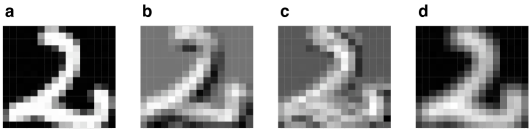
Figure 2: Example of original and filtered digit data. (a) Original digit image. (b & c) Transformed image using two different random local translation-invariant linear filters. (d) Transformed image using a simple local blur filter.

5 Discussion

Our experiments with simulated data suggest that the method performs quite well already for moderate dimensions provided that the noiselevel is not too high. Certainly, the model of drawing $C_{XX}$ according to a distribution that is invariant under $C_{XX}\mapsto UC_{XX}U^{T}$ may be inappropriate for many practical applications. However, as the example with diagonal matrices in Section 1 shows, the statement $\Delta(C_{XX},A)=0$ holds for a much broader class of models. For this reason, the method could also be used as a sanity check for causal hypotheses among one-dimensional variables. Assume, for instance, one has a causal DAG $G$ connecting $2n$ variables attaining values in ${\mathbb{R}}$. If $X_{1},\dots,X_{2n}$ is an ordering that is consistent with $G$, we define $Y:=(X_{1},\dots,X_{n})$ and $W:=(X_{n+1},\dots,X_{2n})$ and check the hypothesis $Y\rightarrow W$ using our method. Provided that the true causal relations are linear, such a hypothesis should be accepted for every possible ordering that is consistent with the true causal DAG. This way one could, for instance, check the causal relation between genes by clustering their expression levels to vector-valued variables.

References

- [1] J. Pearl. Causality: Models, reasoning, and inference. Cambridge University Press, 2000.
- [2] P. Spirtes, C. Glymour, and R. Scheines. Causation, prediction, and search (Lecture notes in statistics). Springer-Verlag, New York, NY, 1993.
- [3] J. Lemeire. Learning causal models of multivariate systems. PhD thesis, Brussels, 2007.
- [4] D. Heckerman, C. Meek, and G. Cooper. A Bayesian approach to causal discovery. In C. Glymour and G. Cooper, editors, Computation, Causation, and Discovery, pages 141–165, Cambridge, MA, 1999. MIT Press.
- [5] J. Mooij, D. Janzing, and B. Schölkopf. Distinguishing between cause and effect, 2008. http://www.causality.inf.ethz.ch/repository.php?id=14.
- [6] Y. Kano and S. Shimizu. Causal inference using nonnormality. In Proceedings of the International Symposium on Science of Modeling, the 30th Anniversary of the Information Criterion, pages 261–270, Tokyo, Japan, 2003.
- [7] S. Shimizu, P. O. Hoyer, A. Hyvärinen, and A. J. Kerminen. A linear non-Gaussian acyclic model for causal discovery. Journal of Machine Learning Research, 7:2003–2030, 2006.
- [8] P. Hoyer, D. Janzing, J. Mooij, J. Peters, and B Schölkopf. Nonlinear causal discovery with additive noise models. In D. Koller, D. Schuurmans, Y. Bengio, and L. Bottou, editors, Advances in Neural Information Processing Systems 21, Vancouver, Canada, 2009. MIT Press.
- [9] K. Zhang and A. Hyvärinen. On the identifiability of the post-nonlinear causal model. In Proc. 25th Conference on Uncertainty in Artificial Intelligence (UAI-2009), 2009. In press.
- [10] J. Lemeire and E. Dirkx. Causal models as minimal descriptions of multivariate systems. http://parallel.vub.ac.be/jan/, 2007.
- [11] D. Janzing and B. Schölkopf. Causal inference using the algorithmic Markov condition. http://arxiv.org/abs/0804.3678, 2008.
- [12] T. Lam. A first course in noncommunitative rings. Springer, 2001.
- [13] M. Ledoux. The concentration of measure phenomenon. Mathematical Surveys and Monographs. American Mathematical Society, 2001.
- [14] Y. Le Cun, B. Boser, J. S. Denker, D. Henderson, R. E. Howard, W. Hubbard, and L. D. Jackel. Handwritten digit recognition with a back-propagation network. In Advances in Neural Information Processing Systems, pages 396–404. Morgan Kaufmann, 1990.