Two-channel model of photoassociation in the vicinity of a Feshbach resonance

Abstract

We derive the two-channel (TC) description of the photoassociation (PA) process in the presence of a magnetic Feshbach resonance and compare to full coupled multi-channel calculations for the scattering of ⁶Li-⁸⁷Rb. Previously derived results [P. Pellegrini et al., Phys. Rev. Lett. 101, 053201 (2008)] are corrected. The PA process is shown to be fully described by two parameters: the maximal transition rate and the point of vanishing transition rate. The TC approximation reproduces excellently the PA transition rates of the full multi-channel calculation and reveals, e.g., that the enhancement of the rate at a resonance is directly connected to the position of vanishing rate. For the description of two independent resonances it was found that only three parameters completely characterize the PA process.

I Introduction

The phenomenon of a magnetic Feshbach resonance (MFR) is widely used for the manipulation of systems of ultracold atoms. One field of interest is the combination of the photoassociation (PA) of molecules with MFRs. It has been shown, both theoretically and experimentally, that the PA transfer rate can be significantly increased in the vicinity of an MFR van Abeelen et al. (1998); Courteille et al. (1998); Grishkevich and Saenz (2007); Junker et al. (2008); Pellegrini et al. (2008). This leads to the prospect of creating a large number of ultracold molecules out of a sample of ultracold atoms. These molecules are of great interest for applications in quantum information processing Micheli et al. (2006); Rabl et al. (2006), the exploration of lattices of dipolar molecules Pupillo et al. (2008), or ultracold chemical reactions Chin et al. (2005); Tscherbul and Krems (2006).

For all PA schemes that exploit the enhancement of PA at an MFR, the understanding of the interplay between both processes is important. Here, we seek to describe the process by a two-channel (TC) approximation Feshbach (1958). In Pellegrini et al. (2008) this approximation has recently been used to predict the behavior of the PA transition rate as a function of the scattering length. We review this approach and find a simplified expression with only two instead of three free parameters. These two parameters which can be, e.g., the maximal transition rate and the position of the minimal transition rate can be obtained either from multi-channel (MC) calculations or from experimental observations. They can serve as a classification of transition processes and reveal a universal dependence of the enhancement of the transition rate on the position of vanishing transition rate.

The Hamiltonian of relative motion for two colliding ground-state alkali-metal atoms is given by Moerdijk and Verhaar (1995)

$$\hat{\rm H}=\hat{\rm T}_{\mu}+\sum_{j=1}^{2}(\hat{\rm V}_{j}^{\rm hf}+\hat{\rm V}_{j}^{\rm Z})+\hat{\rm V}_{\rm int}$$ (1)

where $\hat{\rm T}_{\mu}$ is the kinetic energy and $\mu$ is the reduced mass. The hyperfine operator $\hat{\rm V}_{j}^{\rm hf}=\frac{a_{\rm hf}^{j}}{\hbar^{2}}\vec{s}_{j}\cdot\vec{i}_{j}$ and the Zeeman operator $\hat{\rm V}_{j}^{\rm Z}=(\gamma_{e}\vec{s}_{j}-\gamma_{n}\vec{i}_{j})\cdot\vec{B}$ in the presence of a magnetic field $\vec{B}$ depend on the electronic spin $\vec{s}_{j}$, the nuclear spin $\vec{i}_{j}$, the hyperfine constant $a_{\rm hf}^{j}$ of atom $j=1,2$, and on the nuclear and electronic gyromagnetic factors $\gamma_{n}$ and $\gamma_{e}$. The central interaction

$$\hat{\rm V}_{\rm int}(R)=V_{0}(R)\hat{\rm P}_{0}+V_{1}(R)\hat{\rm P}_{1}$$ (2)

is a combination of singlet and triplet Born-Oppenheimer potentials $V_{0}(R)$ and $V_{1}(R)$ where $\hat{\rm P}_{0}$ and $\hat{\rm P}_{1}$ project respectively on the singlet and triplet components of the scattering wave function.

For low collision energies the eigenfunctions of Hamiltonian (1) may be written as a superposition

$$|\Psi\rangle=\sum_{\alpha}\Psi_{\alpha}(R)|\alpha\rangle$$ (3)

of $s$-wave functions in the atomic basis $|\alpha\rangle=|f_{1},m_{f_{1}}\rangle|f_{2},m_{f_{2}}\rangle$. Here, $\vec{f}_{j}=\vec{s}_{j}+\vec{i}_{j}$ is the total spin of atom $j$ and $m_{f}$ its projection onto the $B$-field axis.

In the following we consider an elastic collision, where only the entrance channel with spin configuration $|\alpha_{0}\rangle$ is open and all other coupled channels are closed.

Within the TC approximation of the scattering process one projects the full MC Hilbert space onto two subspaces, the one of the closed channels (with projection operator $\hat{\rm Q}$) and the one of the open entrance channel (with projection operator $\hat{\rm P}$) Feshbach (1958). The resulting TC Schrödinger equation reads

$$(\hat{\rm H}_{P}-E)|\Psi_{P}\rangle+\hat{\rm W}|\Psi_{Q}\rangle = 0$$ (4)

$$(\hat{\rm H}_{Q}-E)|\Psi_{Q}\rangle+\hat{\rm W}^{\dagger}|\Psi_{P}\rangle = 0\,,$$ (5)

with $\hat{\rm H}_{P}=\hat{\rm P}\hat{\rm H}\hat{\rm P}$, $\hat{\rm H}_{Q}=\hat{\rm Q}\hat{\rm H}\hat{\rm Q}$, $\hat{\rm W}=\hat{\rm P}\hat{\rm H}\hat{\rm Q}$, $|\Psi_{P}\rangle=\hat{\rm P}|\Psi\rangle$ and $|\Psi_{Q}\rangle=\hat{\rm Q}|\Psi\rangle$.

An MFR occurs, if the energy $E$ of the system is close to the eigenenergy $E_{0}$ of a bound state $|\Phi_{b}\rangle$ of the closed-channel subspace. Following the solution in Friedrich (1991) we assume that the closed-channel wave function is simply a multiple $A$ of the bound state $|\Phi_{b}\rangle$, i.e. $|\Psi_{Q}\rangle=A\,|\Phi_{b}\rangle$. This is equivalent to the usual one-pole approximation. Equation (4) may be solved via the Greens operator $\hat{\rm G}_{P}=(E+i\epsilon-\hat{\rm H}_{P})^{-1}$ with $\epsilon\rightarrow 0^{+}$.

The general solution thus reads

$$|\Psi_{P}\rangle = C|\Phi_{\rm reg}\rangle+A\hat{\rm G}_{P}\hat{\rm W}|\Phi_{b}\rangle\,,$$ (6)

$$|\Psi_{Q}\rangle = A|\Phi_{b}\rangle$$ (7)

where $C$ is a normalization constant and $|\Phi_{\rm reg}\rangle$ is the regular solution of $\hat{\rm H}_{P}|\Psi\rangle=E|\Psi\rangle$.

Following the procedure given in Friedrich (1991) one arrives at the closed-channel admixture

$$A=-\tilde{C}\sqrt{\frac{2}{\pi\Gamma}}\sin\delta_{\rm res}\,,$$ (8)

with the normalization constant $\tilde{C}=C/\cos\delta_{\rm res}$. The Greens operator $\hat{\rm G}_{P}$ explicitly given in Friedrich (1991) yields a long range behavior of the open channel

$$\left.\Psi_{P}(R)\right|_{R\rightarrow\infty}=\tilde{C}\sqrt{\frac{2\mu}{\pi\hbar^{2}k}}\sin(kR+\delta_{\rm bg}+\delta_{\rm res})\,.$$ (9)

The total phase shift $\delta=\delta_{\rm bg}+\delta_{\rm res}$ results from the background phase shift $\delta_{\rm bg}$ of the regular solution $|\Phi_{\rm reg}\rangle$, which is connected to the background scattering length $a_{\rm bg}=-\lim_{k\rightarrow 0}\tan{\delta_{\rm bg}}/k$, and a contribution $\delta_{\rm res}$ due to the resonant coupling to the bound state. The resonant phase shift has the functional form

$$\tan\delta_{\rm res}=-\frac{\Gamma/2}{E-E_{\rm R}}$$ (10)

where $E_{R}=E_{0}+\langle\Phi_{b}|\hat{\rm W}^{\dagger}\hat{\rm G}_{P}\hat{\rm W}|\Phi_{b}\rangle$ lies close to the energy of the bound state $E_{0}(B)$. The width of the resonance is given by $\Gamma=2\pi|\langle\Phi_{b}|\hat{\rm W}|\Phi_{\rm reg}\rangle|^{2}$.

One assumes that $E_{R}$ depends approximately linearly on the magnetic field, i.e. for $E\rightarrow 0$ there is some $\sigma$ and $B_{R}$ such that $E_{R}=\sigma(B-B_{R})$. This yields with $\Delta B\equiv\Gamma(2ka_{\rm bg}\sigma)^{-1}$ the well known relation Moerdijk et al. (1995)

$$a_{\rm sc}=a_{\rm bg}\left(1+\frac{\Delta B}{B-B_{R}}\right)$$ (11)

which allows to determine the resonant phase shift

$$\tan\delta_{\rm res}=\frac{ka_{\rm bg}\Delta B}{B_{R}-B}$$ (12)

from experimentally accessible quantities.

Equipped with the MC solution a convenient way to calculate transition rates to molecular bound states is to transform the scattering wave function of Eq. (3) to the molecular basis $|\chi\rangle=|S,M_{S}\rangle|m_{i_{1}},m_{i_{2}}\rangle$ where $S$ and $M_{S}$ are the quantum numbers of the total electronic spin and its projection along the magnetic field and $m_{i_{1}},m_{i_{2}}$ are the nuclear spin projections of the individual atoms.

Within the dipole approximation with electronic dipole transition moment $D(R)$ the free-bound transition rate $\Gamma(B)$ to the final molecular state $|\Psi_{\rm f}\rangle=\frac{\Psi_{\nu}(R)}{R}Y_{J}^{M}(\Theta,\Phi)|\chi_{\rm f}\rangle$ with vibrational quantum number $\nu$ and rotational quantum number $J$ is then proportional to the squared dipole transition moment Sando and Dalgarno (1971)

$$I_{\rm MC}(B)=\left|\int\limits_{0}^{\infty}\Psi_{\nu}(R)D(R)\psi_{\chi_{\rm f}}(R)dR\right|^{2}\,.$$ (13)

Selection rules allow only transitions from the $s$-wave scattering function to a final state with $J=1$. Due to the orthogonality of the molecular basis, only one molecular channel $\psi_{\chi_{\rm f}}(R)$ with the same spin state as the final state has to be considered.

The solutions (6,7) of the TC approximation yield together with the behavior of the closed channel admixture in (8) a squared dipole transition moment

$$I_{\rm TC}(B) = |\langle\Psi_{\rm f}|\hat{\rm D}|\Psi\rangle|^{2}$$ (14)

$$= |\tilde{C}|^{2}\left|C_{1}\cos\delta_{\rm res}-C_{2}\sin\delta_{\rm res}\right|^{2}\,,$$

where $C_{2}=\sqrt{2/\pi\Gamma}(\langle\Psi_{\rm f}|\hat{\rm D}\hat{\rm G}_{P}\hat{\rm W}|\Phi_{b}\rangle+\langle\Psi_{\rm f}|\hat{\rm D}|\Phi_{b}\rangle)$ and $C_{1}=\langle\Psi_{\rm f}|\hat{\rm D}|\Phi_{\rm reg}\rangle$ do not vary with the magnetic field $B$. The prefactor $\tilde{C}$ may vary with $a_{\rm sc}$. However, in the following we consider energy-normalized scattering solutions with $\tilde{C}\equiv 1$. Introducing $\beta=|\tilde{C}|^{2}(C_{1}^{2}+C_{2}^{2})$ and $\tan\delta_{0}=C_{1}/C_{2}$ one can further simplify Eq. (14) to

$$I_{\rm TC}(B)=\beta\sin^{2}\left(\delta_{\rm res}-\delta_{0}\right)\,.$$ (15)

Due to the low-energy behavior of the regular solution $\Gamma\propto k$ and $C_{1}\propto\sqrt{k}$ holds for $k\rightarrow 0$ Moerdijk and Verhaar (1995). Therefore one can associate a finite length

$$a_{e}=-\lim_{k\rightarrow 0}\frac{\tan\delta_{0}}{k}$$ (16)

with the phase shift $\delta_{0}$.

Let us point out some differences to the previously derived result for the dipole transition moment in Pellegrini et al. (2008). In the notation of the current work Eq. (8) in Pellegrini et al. (2008) gives

$$I_{\rm TC}(B)=K|1+C_{1}\tan\delta_{\rm res}+C_{2}\sin\delta_{\rm res}|^{2}$$ (17)

with $K=|\langle\Psi_{\rm f}|\hat{\rm D}|\Phi_{\rm reg}\rangle|^{2}$, $C_{1}=\langle\Psi_{\rm f}|\hat{\rm D}|\Phi_{\rm irr}\rangle/\langle\Psi_{\rm f}|\hat{\rm D}|\Phi_{\rm reg}\rangle$, and $C_{2}=-\sqrt{2/\pi\Gamma}\langle\Psi_{\rm f}|\hat{\rm D}|\Phi_{b}\rangle/\langle\Psi_{\rm f}|\hat{\rm D}|\Phi_{\rm reg}\rangle$. The most obvious difference to Eq. (14) is the dependence on three parameters $K,C_{1}$ and $C_{2}$ and not just two. This is a result of an inconsistent normalization of open and closed channels in Pellegrini et al. (2008). The open channel was not energy normalized and leads thus to a term proportional to $\tan\delta_{\rm res}$. Furthermore, the open channel was described as a pure sum of regular and irregular solution. This may, however, only be done for interatomic distances, were the coupling to the closed channels induced by the exchange energy is negligible. A fit of Eq. (17) to a full MC calculation seemed to be nevertheless possible which might however be the result of the freedom of three fitting parameters.

The universal dependence of the PA transition rates on just two parameters in Eq. (15) reveals an important physical aspect. The enhancement of the transition rate is directly connected to the position of vanishing transition rate. On the one hand the transition rate is vanishing at a scattering length $a_{\rm sc}^{({\rm min})}=a_{\rm bg}+a_{e}$ or at a corresponding magnetic field

$$B_{\rm min}=B_{R}+\Delta B\frac{a_{\rm bg}}{a_{e}}\,.$$ (18)

On the other hand the point of vanishing transition rate is connected to the enhancement ratio

$$\frac{\Gamma_{\rm max}}{\Gamma_{\rm bg}}=\frac{1}{\sin^{2}\delta_{0}}\approx\frac{1}{k^{2}a_{e}^{2}}=\left(\frac{B_{\rm min}-B_{R}}{k\,a_{\rm bg}\Delta B}\right)^{2}$$ (19)

of the maximum transition rate $\Gamma_{\rm max}$ and the background rate $\Gamma_{\rm bg}$ in the presence of an off-resonant magnetic field (i.e. where $\delta_{\rm res}=0$).

In order to verify the TC description of the PA process, we consider the exemplary case of an elastic collision of ⁶Li-⁸⁷Rb (⁶Li is atom 1, ⁸⁷Rb is atom 2) in the initial atomic basis state $|\alpha_{0}\rangle=|1/2,1/2\rangle|1,1\rangle$. For an energy 50 Hz above the threshold of the entrance channel which is well in the $s$-wave scattering regime the MC solution was calculated for different magnetic fields $B$ in Grishkevich et al. . For $B<1500\,$G two $s$-wave resonances occur, a broad one at $B=1066,917\,$G which was also observed experimentally Deh et al. (2008), and a narrow one at $B=1282.576\,$G. The dependence of the scattering length $a_{\rm sc}$ on the magnetic field strength is shown in Fig. 1.

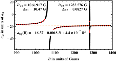
Figure 1: (Color online) Scattering length $a_{\rm sc}$ as a function of the external magnetic field value $B$ for ⁶Li-⁸⁷Rb scattering at $E=50\,$Hz (dots). A fit according to Eq. (20) is depicted by the solid (red) line. The value of $a_{\rm bg}(B)$ is shown by the dashed (orange) line. All fitting parameters are shown in the plot.

Assuming that the two resonances are sufficiently separated in order to describe the process by two independent resonances one may generalize Eq. (11) to

$$a_{\rm sc}(B)=a_{\rm bg}\left(1+\frac{\Delta B_{1}}{B-B_{R1}}+\frac{\Delta B_{2}}{B-B_{R2}}\right)\,.$$ (20)

Additionally, we account for effects beyond the one-pole approximation by allowing $a_{\rm bg}$ to vary slowly with $B$ as $a_{\rm bg}(B)=a_{0}+a_{1}\cdot B+a_{2}\cdot B^{2}$. With this quadratic expansion, a fit according to Eq. (20) excellently reflects the MC behavior as shown in Fig. 1.

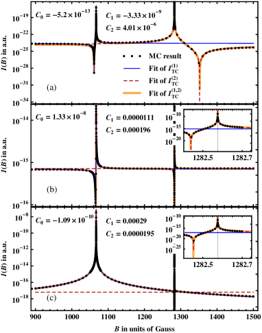
Figure 2: (Color online) Squared dipole transition moment as a function of the external magnetic field for ⁶Li-⁸⁷Rb scattering at $E=50\,$Hz (dots). Transitions to the molecular singlet state $|0,0\rangle|0,3/2\rangle$ (a) and the triplet states $|1,-1\rangle|1,3/2\rangle$ (b) and $|1,1\rangle|1,-1/2\rangle$ (c) are considered. In each graph a fit according to Eq.s (21) and (22) is performed and the resulting fitting parameters for Eq. (21) are shown. The insets focus respectively on a region $B_{R2}-2\Delta B_{2}\leq B\leq B_{R2}+2\Delta B_{2}$.

We consider the exemplary case of a dipole transitions of the scattering state to the absolute vibrational ground state of the electronic singlet configuration $X^{1}\Sigma^{+}$ and the triplet configuration $a^{3}\Sigma^{+}$. These transitions take place at internuclear distances where the coupling between all atomic channels is strong such that any deficiency of the TC description would become obvious. The MC rate was calculated in Grishkevich et al. for an electronic dipole moment in the linear approximation $D(R)=D_{0}+D_{1}\cdot R$, where $D_{0}$ could be neglected. In the following we use $D_{0}=0$ and $D_{1}=E_{h}/a_{0}$. The magnetic field dependence of the according dipole transition moment to ground states in different spin configurations is shown in Fig. 2.

We fit the MC behavior by assuming again that the two resonances are sufficiently separated, such that one can add the transition amplitudes $A_{\rm TC}^{(j)}(B)=C_{0}\cos(\delta_{\rm res}^{(j)})-C_{j}\sin(\delta_{\rm res}^{(j)})$ of both resonances $j=1,2$ independently and take the absolute square of the sum

$$I_{\rm TC}^{(1,2)}(B)=|A_{\rm TC}^{(1)}(B)+A_{\rm TC}^{(2)}(B)|^{2}\,$$ (21)

in order to determine the dipole transition moment. The resonant phase shifts $\tan\delta_{\rm res}^{(j)}=ka_{\rm bg}(B)\Delta B_{j}/(B_{Rj}-B)$ for $j=1,2$ are in analogy to Eq. (12) associated to the resonant coupling to two different closed-channel bound states. Since $C_{0}$ does not depend on the resonant molecular bound state $|\Phi_{b}\rangle$, it is independent of the magnetic field $B$. Hence, for describing a transition process to a specific molecular state for two well separated resonances, one needs only three independent parameters.

Additionally a fit to the behavior

$$I_{\rm TC}^{(j)}(B)=\beta_{j}\sin^{2}(\delta_{\rm res}^{(j)}-\delta_{0}^{(j)})$$ (22)

for $j=1,2$ is performed which neglects respectively one resonance. Again one can connect the phase shifts $\delta_{0}^{(j)}$ to the corresponding lengths $a_{e}^{(j)}$ via Eq. (16) which allows also to validate the applicability of Eq. (19) for both resonances separately.

Considering Fig. 2 one finds that for all shown transitions the TC approximation for two well separated resonances excellently describes the magnetic-field dependence of the MC transition rate. The behavior of Eq. (22) reproduces each of the MC resonances $j=1,2$ in an interval of several $\Delta B_{j}$ around the resonant magnetic fields $B_{Rj}$. With only one parameter more than for the description of a single resonance, both resonances can be well described by Eq. (21). This is remarkable, since the behavior of the transition rates to all four different spin configurations are quite different. Nevertheless all features are reproduced by just three parameters.

Table 1: Enhancement of the dipole transition rate between off-resonant and resonant magnetic field in MC and TC description for transitions to all eight possible spin states $|S,M_{S}\rangle|m_{i_{1}},m_{i_{2}}\rangle$ at the two resonances at $B_{R1}=1066,917\,$G and $B_{R2}=1282.576\,$G.

Molecular	Resonance 1		Resonance 2
state	$I_{\rm MC}^{\rm max}/I_{\rm MC}^{\rm off}$	$(k\,a_{e}^{(1)})^{-2}$	$I_{\rm MC}^{\rm max}/I_{\rm MC}^{\rm off}$	$(k\,a_{e}^{(2)})^{-2}$
$|0,0\rangle\phantom{}|0,\frac{3}{2}\rangle$	$5.81\cdot 10^{6}$	$5.83\cdot 10^{6}$	$6.85\cdot 10^{12}$	$1.39\cdot 10^{13}$
$|0,0\rangle\phantom{}|1,\frac{1}{2}\rangle$	$2.62\cdot 10^{8}$	$3.49\cdot 10^{8}$	$6.57\cdot 10^{6}$	$1.27\cdot 10^{7}$
$|1,-1\rangle|1,\frac{3}{2}\rangle$	$1.80\cdot 10^{5}$	$1.75\cdot 10^{5}$	$5.73\cdot 10^{7}$	$5.41\cdot 10^{7}$
$|1,0\rangle\phantom{}|0,\frac{3}{2}\rangle$	$8.86\cdot 10^{6}$	$8.69\cdot 10^{6}$	$1.63\cdot 10^{13}$	$5.93\cdot 10^{13}$
$|1,0\rangle\phantom{}|1,\frac{1}{2}\rangle$	$5.04\cdot 10^{9}$	$2.14\cdot 10^{9}$	$2.15\cdot 10^{8}$	$4.71\cdot 10^{7}$
$|1,1\rangle\phantom{}|-1,\frac{3}{2}\rangle$	$5.77\cdot 10^{6}$	$8.41\cdot 10^{6}$	$7.76\cdot 10^{12}$	$5.21\cdot 10^{13}$
$|1,1\rangle\phantom{}|0,\frac{1}{2}\rangle$	$1.88\cdot 10^{7}$	$2.13\cdot 10^{7}$	$1.32\cdot 10^{13}$	$6.57\cdot 10^{13}$
$|1,1\rangle\phantom{}|1,-\frac{1}{2}\rangle$	$1.09\cdot 10^{10}$	$1.18\cdot 10^{12}$	$3.66\cdot 10^{7}$	$4.41\cdot 10^{7}$

The good description of the MC transition rates by Eq. (22) suggests that Eq. (19) indeed reflects the dependence of the PA enhancement on the position of vanishing transition rate. In Eq. (19) the enhancement was defined relative to the transition rate at the background scattering length. This point is reached, however, only at infinite detuning from the resonant magnetic field $B_{R}$. In order to nevertheless verify the validity of Eq. (19) we relate the maximal transition rate $I_{\rm MC}^{\rm max}$ at each resonance separately to the transition rate $I_{\rm MC}^{\rm off}=I_{\rm MC}(800\,{\rm G})$ far away from both resonances. We do not choose a magnetic field with larger detuning to avoid effects of other resonant molecular bound states. In Tab. 1 the ratio $I_{\rm MC}^{\rm max}/I_{\rm MC}^{\rm off}$ is compared for both resonances to the prediction of Eq. (19) for transitions to the vibrational ground states of all eight possible spin configurations in the molecular basis. One finds that the order of magnitude generally agrees excellently. Only for few transitions such as the one to the molecular states $|1,1\rangle|1,-1/2\rangle$ at the first (broad) resonance the orders of magnitude differ significantly. A view on Fig. 2 (c) reveals that this is not related to a break down of Eq. (19), but that the absence of a vanishing transition rate leads to a comparably slow degradation of the transition rate such that $I_{\rm MC}^{\rm off}$ is not a good representation for the background transition rate. On the other hand, for transitions for which the background transition rate is quickly approached when detuning from the resonance, the two estimates of the enhancement agree even to the first significant digit (see the third row in Tab. 1 and the corresponding Fig. 2 (b)). This and the results above demonstrate that the TC approximation provides an excellent basis to understand PA processes in the presence of an external magnetic field inducing an MFR.

We thank Y. V. Vanne for fruitful discussions and for providing us with the differential MC transition rates of Grishkevich et al. . The authors are grateful to the Deutsche Forschungsgemeinschaft (SFB 450 C6) for financial support.

References

- van Abeelen et al. (1998) F. A. van Abeelen, D. J. Heinzen, and B. J. Verhaar, Phys. Rev. A 57, R4102 (1998).
- Courteille et al. (1998) P. Courteille, R. S. Freeland, D. J. Heinzen, F. A. van Abeelen, and B. J. Verhaar, Phys. Rev. Lett. 81, 69 (1998).
- Grishkevich and Saenz (2007) S. Grishkevich and A. Saenz, Phys. Rev. A 76, 022704 (2007).
- Junker et al. (2008) M. Junker, D. Dries, C. Welford, J. Hitchcock, Y. Chen, and R. Hulet, Phys. Rev. Lett. 101, 060406 (2008).
- Pellegrini et al. (2008) P. Pellegrini, M. Gacesa, and R. Côté, Phys. Rev. Lett. 101, 053201 (2008).
- Micheli et al. (2006) A. Micheli, G. K. Brennen, and P. Zoller, Nature 2, 341 (2006).
- Rabl et al. (2006) P. Rabl, D. DeMille, J. M. Doyle, M. D. Lukin, R. J. Schoelkopf, and P. Zoller, Phys. Rev. Lett. 97, 033003 (2006).
- Pupillo et al. (2008) G. Pupillo, A. Griessner, A. Micheli, M. Ortner, D.-W. Wang, and P. Zoller, Phys. Rev. Lett. 100, 050402 (2008).
- Chin et al. (2005) C. Chin, T. Kraemer, M. Mark, J. Herbig, P. Waldburger, H.-C. Nägerl, and R. Grimm, Phys. Rev. Lett. 94, 123201 (2005).
- Tscherbul and Krems (2006) T. V. Tscherbul and R. V. Krems, Phys. Rev. Lett. 97, 083201 (2006).
- Feshbach (1958) H. Feshbach, Ann. Phys. (N.Y.) 5, 357 (1958).
- Moerdijk and Verhaar (1995) A. J. Moerdijk and B. J. Verhaar, Phys. Rev. A 51, R4333 (1995).
- Friedrich (1991) H. Friedrich, Theoretical Atomic Physics (Springer-Verlag, Berlin, 1991).
- Moerdijk et al. (1995) A. J. Moerdijk, B. J. Verhaar, and A. Axelsson, Phys. Rev. A 51, 4852 (1995).
- Sando and Dalgarno (1971) K. Sando and A. Dalgarno, Mol. Phys. 20, 103 (1971).
- (16) S. Grishkevich, P.-I. Schneider, Y. Vanne, and A. Saenz, to be published.
- Deh et al. (2008) B. Deh, C. Marzok, C. Zimmermann, and P. W. Courteille, Phys. Rev. A 77, 010701 (2008).