Ballistic quantum spin Hall state and enhanced edge backscattering
in strong magnetic fields

Abstract

The quantum spin Hall (QSH) state, observed in a zero magnetic field in HgTe quantum wells, respects the time-reversal symmetry and is distinct from quantum Hall (QH) states. We show that the QSH state persists in strong quantizing fields and is identified by counter-propagating (helical) edge channels with nonlinear dispersion inside the band gap. If the Fermi level is shifted into the Landau-quantized conduction or valence band, we find a transition between the QSH and QH regimes. Near the transition the longitudinal conductance of the helical channels is strongly suppressed due to the combined effect of the spectrum nonlinearity and enhanced backscattering. It shows a power-law decay $B^{-2N}$ with magnetic field $B$, determined by the number of backscatterers on the edge, $N$. This suggests a rather simple and practical way to probe the quality of recently realized quasiballistic QSH devices using magnetoresistance measurements.

Introduction.- Recently novel two-dimensional (2D) electronic state - quantum spin Hall (QSH) state - has been theoretically proposed Kane and Mele (2005); Bernevig et al. (2006); Murakami (2006) and experimentally realized in HgTe quantum wells (QWs) König et al. (2007, 2008); Roth et al. (2009). It originates from spin-orbit band splitting and is characterized by time-reversal invariant gapless states on sample edges, where electrons with opposite spins counter-propagate, while the bulk states are fully gapped. Such (helical) edge channels make the QSH insulators topologically distinct from ordinary band insulators, and hold promise for reversible manipulation of spin-dependent quantum transport. Similar edge states and transport have been discussed in the quantum Hall regime in graphene Abanin et al. (2006, 2007); Nomura and MacDonald (2006); Sheng et al. (2005); Shimshoni et al. (2009).

In experiments on HgTe QWs König et al. (2007, 2008), the QSH regime was detected by measuring the longitudinal conductance of two spin channels propagating in the same direction on opposite edges of the sample. This finding was further substantiated by the observed suppression of the edge transport in a magnetic field König et al. (2007, 2008), which breaks the time-reversal symmetry of the QSH state, thus revealing the helical edge channels. The magnetoresistance measurements König et al. (2007, 2008) and theory Maciejko et al. have so far been done for large disordered samples. In view of the progress in the miniaturization of the QSH devices Roth et al. (2009) there is an apparent need to investigate the magnetotransport in the ballistic QSH regime, which is the goal of our work.

The interest in the ballistic QSH transport originates from the profound difference between the helical edge states, characterized by the dissipative longitudinal conductance $\sim 2e^{2}/h$ König et al. (2007, 2008); Roth et al. (2009), and dissipationless chiral quantum Hall (QH) channels Halperin (1982); MacDonald and Streda (1984). As a new test to demonstrate this distinction, we propose to measure the longitudinal magnetoconductance of a ballistic HgTe QW when its edge spectrum changes from helical to chiral. Such a transition is expected when the Fermi level is driven from the band gap into the Landau-quantized conduction or valence band where a dissipationless QH state sets in. The latter is insensitive to the edge backscattering Halperin (1982); MacDonald and Streda (1984), while on the QSH side of the transition we find strong suppression of the two-terminal conductance $g$ due to the backscattering in a magnetic field $B$:

$$g(\epsilon,B)\propto(E_{g}-|\epsilon|)^{2N}/B^{2N},\quad|\epsilon|\to E_{g}.$$ (1)

Here $\epsilon$ indicates the position of the Fermi level with respect to the middle of the band gap (equal to $2E_{g}$). This result contrasts the zero-field conductance which increases as the Fermi energy is pushed into the metallic-type conduction or valence band König et al. (2007, 2008); Roth et al. (2009). Also, unlike the exponential $B$ decay in strongly disordered systems Maciejko et al. , Eq. (1) describes a power-law magnetoconductance.

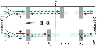
Figure 1: (Color online) Two-terminal QSH device in a strong magnetic field. Edge channels are localized within the magnetic length $\lambda$. Gray regions schematically indicate backscattering centers (see, also, Eq. (20)). We assume that the current is carried by the right moving states (solid arrows $\pm$), populated in contact L and equilibrating in contact R.

Equation (1) assumes the presence of a few ($N$) backscattering centers (see, also, Fig. 1), such as sample inhomogeneities where electronic trap states can interact with the edge channels randomizing their propagation directions Roth et al. (2009). Although in a zero field this effect is believed to be weak, we show that near the QSH-QH transition the backscattering is dramatically enhanced due to the reduction of the group velocities of the coupled QSH modes. According to Eq. (1), the analysis of the power of the magnetoconductance decay can be a simple tool to determine the quality of the QSH devices, which is an important practical task.

Model.- We will first analyze the edge states in scattering-free HgTe QWs using the effective 4-band model derived in Refs. Bernevig et al. (2006); König et al. (2008). In this approach one works in the basis of the four states near the $\Gamma$ (${\bf k}=0$) point of the Brillouin zone: $|e_{1}+\rangle$, $|h_{1}+\rangle$, $|e_{1}-\rangle$, and $|h_{1}-\rangle$, where $e_{1}$ and $h_{1}$ are the s-like electron and p-like hole QW subbands, respectively. The index $\tau=\pm$ accounts for the spin degree of freedom. The effective two-dimensional Hamiltonian can be approximated by a diagonal matrix in ${\tau}$ space Bernevig et al. (2006); König et al. (2008):

$$H=\left(\begin{matrix}h_{\bf k}&0\\ 0&h^{\ast}_{\bf-k}\\ \end{matrix}\right),h_{\bf k}={\bf d}_{\bf k}\mbox{\boldmath$\sigma$},\,{\bf d}_{\bf k}=(\hbar\upsilon k_{x},-\hbar\upsilon k_{y},M).$$ (2)

where Pauli matrices $\sigma_{x,y,z}$ act in subband space, $\upsilon\approx 5.5\times 10^{5}$ms^-1 is the effective velocity König et al. (2008), and $M$ determines the band gap $E_{g}=|M|$ at ${\bf k}=0$. In Eq. (2) we omit terms $\propto{\bf k}^{2}$ which are small near the $\Gamma$ point and in the range of fields we consider Schmidt et al. (2009). We also neglect the bulk inversion asymmetry because we will focus on strong magnetic fields where the subband mixing is suppressed. Up to a unitary transformation, Eq. (2) is equivalent to a massive Dirac Hamiltonian $H_{D}=\hbar\upsilon\tau_{z}\mbox{\boldmath$\sigma$}{\bf k}+M\tau_{z}\sigma_{z}$ [$\tau_{z}$ is the Pauli matrix in spin space]. We will work with the corresponding retarded Green’s function defined by $[\epsilon\,I-H_{D}]{\hat{G}}({\bf r},{\bf r}^{\prime})=I\delta({\bf r}-{\bf r}^{\prime}),$ where ${\bf k}=-i{\bf\nabla}-e{\bf A}({\bf r})/c\hbar,$ ${\bf A}({\bf r})=(-By,0,0)$ is the vector potential of an external magnetic field $B$, and $I=\tau_{0}\sigma_{0}={\rm diag}(1,1,1,1)$. Assuming a sufficiently wide sample, we find ${\hat{G}}({\bf r},{\bf r}^{\prime})$ near one of the edges, e.g. $y=0$, using the boundary condition ${\hat{G}}({\bf r},{\bf r}^{\prime})|_{y=0}=\tau_{0}\sigma_{x}\,{\hat{G}}({\bf r},{\bf r}^{\prime})|_{y=0},$ equivalent to confinement by infinite ”mass” at $y<0$ Berry and Mondragon (1987), . The matrix ${\hat{G}}={\rm diag}({\hat{G}}_{+},{\hat{G}}_{-})$ is diagonal in $\tau$ space, and each ${\hat{G}}_{\tau}$ can be diagonalized in e,h space:

$${\hat{G}}_{\tau}=\left(\begin{array}[]{cc}1&\frac{\upsilon(p_{x}-ip_{y})}{\tau\epsilon-M}\\ \frac{\upsilon(p_{x}+ip_{y})}{\tau\epsilon+M}&1\end{array}\right)\left(\begin{array}[]{cc}G_{ee|\tau}&0\\ 0&G_{hh|\tau}\end{array}\right).$$ (7)

Expanding ${\hat{G}}$ in plane waves ${\rm e}^{ikx}$ yields the boundary problem for the diagonal elements:

$$\left[\partial^{2}_{z}-\frac{(z-z_{k})^{2}}{4}-a\right]G_{ee|\tau k}=\frac{\lambda(\epsilon+\tau M)}{\hbar^{2}\upsilon^{2}}\delta(z-z^{\prime}),$$ (8)

$$\left.\partial_{z}G_{ee|\tau k}=q\,G_{ee|\tau k}\right|_{z=0},\,q=\frac{\lambda(\tau\varepsilon+M)}{\hbar\upsilon}-\lambda k,$$ (9)

with $z=y/\lambda$, $z_{k}=-2\lambda\,k\,{\rm sgn}(eB)$, $\lambda=\sqrt{c\hbar/2|eB|}$, and $a=\lambda^{2}(M^{2}-\epsilon^{2})/\hbar^{2}\upsilon^{2}-\,{\rm sgn}(eB)/2$. For $G_{hh|\tau k}$ one replaces $\tau,k,B\to-\tau,-k,-B$. The solution is obtained in terms of the parabolic cylinder function $U(a,z)$ . It contains the edge contribution of the following form:

$$\hat{G}_{\tau k}=\frac{\alpha(z,z^{\prime})\left(\begin{array}[]{cc}1&\beta(z^{\prime})\\ \beta(z)&\beta(z)\beta(z^{\prime})\end{array}\right)}{\epsilon-\tau M-\tau(\hbar v/\lambda)U(a,-z_{k})/U(a+1,-z_{k})},$$ (12)

$$\alpha=\frac{U(a,z-z_{k})U(a,z^{\prime}-z_{k})}{\lambda U(a,-z_{k})U(a+1,-z_{k})},\beta=\frac{U(a,-z_{k})U(a+1,z-z_{k})}{U(a+1,-z_{k})U(a,z-z_{k})}.$$ (13)

The new feature of this solution is that it is valid for an arbitrary parameter $\hbar\upsilon/\lambda|M|$ which measures the magnetic field strength. Below we compare weak- and strong-field regimes defined by $\hbar\upsilon/\lambda|M|\leq 1$ and $\hbar\upsilon/\lambda|M|\gg 1$.

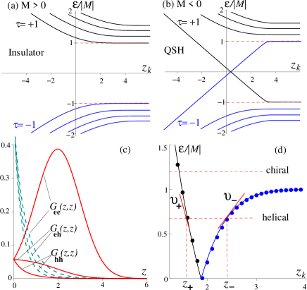
Figure 2: (Color online) Edge-state energy vs. center-of-oscillator coordinate $z_{k}=-2\lambda\,k\,{\rm sgn}(eB)$ [$\hbar\upsilon/\lambda|M|=0.5$, $eB>0$]: (a) insulator and (b) QSH state with two counterpropagating gapless spin channels. (c) Spatial behavior of zero-energy states in weak (dashed curves) and strong (solid curves) fields [see, Eq. (12) and text], (d) Numerical (points) and analytical (Eq. 17, solid lines) results for the spectrum in strong fields, $\hbar\upsilon/\lambda|M|\geq 10$. It transforms from helical to chiral at $\epsilon=|M|$.

Weak- vs. strong-field QSH channels.- The edge-state spectrum is given by the pole of Eq. (12). For weak fields we reproduce the transition from the band insulator with $M>0$ to the QSH state with $M<0$ [cf. Figs. 2(a) and (b)], which is observed at the critical QW thickness $\approx 6.3$ nm Bernevig et al. (2006); König et al. (2007, 2008). The QSH state has two gapless counter-propagating spin modes exponentially localized at the edge Bernevig et al. (2006); Zhou et al. (2008), as seen from Eq. (12) and Fig. 2(c) where we use the asymptotic formula $U(a,z)\approx\sqrt{\pi}/[2^{a/2+1/4}\Gamma(3/4+a/2)]{\rm e}^{-\sqrt{a}\,z}$ with $|a|\gg 1$ Abramowitz and Stegun (1964), valid for low fields and energies $|\epsilon|<|M|$:

$${\hat{G}}_{\tau k}\approx\frac{(\sigma_{0}+\sigma_{x})\,\frac{|M|}{\hbar\upsilon}{\rm e}^{-|M|(y+y^{\prime})/\hbar\upsilon}}{\epsilon-\tau M\Theta(M)-\tau\hbar\upsilon(k-k_{B})},\,\frac{\hbar\upsilon}{\lambda|M|}\ll 1.$$ (14)

The subgap dispersion is linear: $\epsilon_{\tau k}=\tau\hbar\upsilon(k-k_{B})$ for $M<0$. The magnetic field only shifts the zero-energy point $k_{B}=-eB\upsilon/(2c|M|)$ with no effect on transport.

As the magnetic field does not open a gap, the QSH state persists in strong fields $\hbar\upsilon/\lambda|M|\gg 1$, though the QSH channels are no longer localized at the edge [see, solid curves in Fig. 2(c)]. The electron function $G_{ee}(z,z)\propto\alpha(z,z)$ for $eB>0$ [or the hole one $G_{hh}(z,z)$ for $eB<0$] behaves almost like the lowest-Landau-level bulk wave function peaked at the center of oscillator (COS) $z_{k}$. The other functions are small at $z\sim z_{k}$. The strong-field asymptotic is obtained for $U(a,z)\approx U(-1/2,z)={\rm e}^{-z^{2}/4}$, $U(a+1,z)\approx U(1/2,z)={\rm e}^{z^{2}/4}\sqrt{\pi/2}\,{\rm erfc}(z/\sqrt{2})$, and $\beta\ll 1$ in Eqs. (12) and (13):

$${\hat{G}}_{\tau k}\approx\frac{\sigma_{0}+\sigma_{z}}{2}\,G_{\tau k},\qquad G_{\tau k}(z,z^{\prime})=\frac{\alpha(z,z^{\prime})}{\epsilon-\epsilon_{\tau k}},$$ (15)

$$\alpha(z,z^{\prime})\approx\sqrt{\frac{2}{\pi}}\frac{{\rm e}^{-\frac{(z-z_{k})^{2}}{4}-\frac{(z^{\prime}-z_{k})^{2}}{4}}}{\lambda\,{\rm erfc}(-z_{k}/\sqrt{2})},$$ (16)

$$\epsilon_{\tau k}=\tau M+\tau\sqrt{\frac{2}{\pi}}\,\frac{\hbar\upsilon}{\lambda}\frac{{\rm e}^{-z_{k}^{2}/2}}{{\rm erfc}(-z_{k}/\sqrt{2})},\quad\frac{\hbar\upsilon}{\lambda|M|}\gg 1,\quad\quad$$ (17)

where ${\rm erfc}(z)$ is the complementary error function. However, the most essential distinction of this regime is the nonlinear spectrum (17). Upon crossing the gap energy $E_{g}=|M|$ it changes from helical to chiral, as illustrated in Fig. 2(d). Therefore, the QSH state transforms into a dissipationless $\nu=1$ QH state Halperin (1982); MacDonald and Streda (1984). Unlike related work on HgTe QWs König et al. (2008); Schmidt et al. (2009); Akhmerov et al. (2009) and graphene Abanin et al. (2006); Shimshoni et al. (2009), we intend to study the QSH-QH transition in the energy (e.g. gate voltage) dependence of the longitudinal conductance. For that purpose, we need the group velocities, $\upsilon_{\pm}(\epsilon,B)$ and COS coordinates, $z_{\pm}(\epsilon,B)$, which are obtained from Eq. (17) linearized near given energy, $\epsilon_{\tau k}\approx\epsilon-(\hbar\upsilon_{\tau}/2\lambda)(z_{k}-z_{\tau})$. Here $z_{\tau}(\epsilon,B)$ is the solution of equation $\epsilon_{\tau k}=\epsilon$, which is related to the velocity by

$$\upsilon_{\tau}(\epsilon,B)=2\lambda(\tau|M|+\epsilon)\,z_{\tau}(\epsilon,B)/\hbar.$$ (18)

The edge state can be described by the one-dimensional Green’s function, $G_{\tau}(x,x^{\prime})=\int\frac{dk}{2\pi}\,e^{ik(x-x^{\prime})}$ $\times\int_{0}^{\infty}dy\,G_{\tau k}(y,y)$, where $G_{\tau k}(y,y)$ is localized within $\lambda$ [see, Eq. (16)]. Using the linearized dispersion we find

$$G_{\tau}(x,x^{\prime})=\frac{{\rm e}^{ik_{\tau}(\epsilon,B)(x-x^{\prime})}}{i\hbar|\upsilon_{\tau}(\epsilon,B)|}\Theta([x-x^{\prime}]\tau),k_{\tau}=-\frac{z_{\tau}}{2\lambda}.$$ (19)

The step function $\Theta([x-x^{\prime}]\tau)$ accounts for the chirality.

Edge backscattering and magnetoconductance.- We now calculate the two-terminal conductance of a QSH system [see, Fig. 1] using the scattering matrix formalism. Since the edges are assumed decoupled, it is sufficient to do the calculations for one of them, e.g., for the lower edge in Fig. 1 which is described by the following ${\hat{S}}$ matrix: ${\hat{S}}=\bigl{(}\begin{smallmatrix}r^{-+}_{{}_{LL}}&t^{--}_{{}_{LR}}\\ t^{++}_{{}_{RL}}&r^{+-}_{{}_{RR}}\\ \end{smallmatrix}\bigr{)}\otimes\frac{\sigma_{0}+\sigma_{z}}{2}.$ Here $r$’s and $t$’s are the reflection and transmission amplitudes for the right (”+”)- and left (”-”) -moving states; $(\sigma_{0}+\sigma_{z})/2$ projects the ${\hat{S}}$ matrix on the electron QW subband which has the non-vanishing wave function [see, Eq. (15)]. The conductance, $g=(e^{2}/h)\left|t^{++}_{{}_{RL}}\right|^{2},$ is calculated using Fisher-Lee relation Fisher and Lee (1981), $t^{++}_{{}_{RL}}=i\hbar|\upsilon_{+}|{\cal G}_{++}(x\in R,x^{\prime}\in L),$ between $t^{++}_{{}_{RL}}$ and the diagonal element ${\cal G}_{++}(x,x^{\prime})$ of the Green’s function ${\cal\hat{G}}(x,x^{\prime})=\bigl{(}\begin{smallmatrix}{\cal G}_{++}&{\cal G}_{+-}\\ {\cal G}_{-+}&{\cal G}_{--}\end{smallmatrix}\bigr{)}.$ Its off-diagonal part is due to backscattering. We model it by the sum of $N$ potentials, localized at positions $x_{n}$ with non-zero matrix elements $V_{n}$ between the right- and left-moving states:

$${\hat{V}}(x)=\sum\nolimits_{n=1..N}V_{n}\delta(x-x_{n})\,\tau_{x}.$$ (20)

Microscopically, the coupling between the counter-propagating channels can be mediated by interaction with electronic trap states which are likely to exist even in high quality samples Roth et al. (2009). Note that choosing the other off-diagonal matrix, $\tau_{y}$ does not change the final result. Potential (20) results in the Dyson equation ${\cal\hat{G}}(x,x^{\prime})={\hat{G}}(x,x^{\prime})+\sum_{n=1..N}{\hat{G}}(x,x_{n})V_{n}\,\tau_{x}\,{\cal\hat{G}}(x_{n},x^{\prime})$. This allows us to express the off-diagonal part ${\cal G}_{\tau,-\tau}(x,x^{\prime})$ through ${\cal G}_{\tau\tau}(x,x^{\prime})$ and obtain a closed equation for the latter: ${\cal G}_{\tau\tau}(x,x^{\prime})=G_{\tau}(x,x^{\prime})++\sum_{n,m=1..N}G_{\tau}(x,x_{n})V_{n}G_{-\tau}(x_{n},x_{m})V_{m}{\cal G}_{\tau\tau}(x_{m},x^{\prime}).$ With known unperturbed function $G_{\tau}$ (19) and for not large $N$, we solve this equation and calculate $g$. Let us look first at the particular cases $N=1,2$ and $3$:

$$g=\frac{e^{2}}{h}\bigl{(}1+\frac{V_{1}^{2}}{\hbar^{2}|\upsilon_{+}\upsilon_{-}|}\bigr{)}^{-2},$$ (21)

$$g=\frac{e^{2}}{h}\bigl{|}1+\frac{V^{2}_{1}+V^{2}_{2}+V_{1}V_{2}{\rm e}^{iQd_{12}}}{\hbar^{2}|\upsilon_{+}\upsilon_{-}|}+\frac{V^{2}_{1}V^{2}_{2}}{\hbar^{4}\upsilon^{2}_{+}\upsilon^{2}_{-}}\bigr{|}^{-2},$$ (22)

$$g=\frac{e^{2}}{h}\Bigl{|}1+\frac{\sum\limits_{n=1}^{3}V^{2}_{n}+V_{1}V_{2}{\rm e}^{iQd_{12}}+V_{1}V_{3}{\rm e}^{iQd_{13}}+V_{2}V_{3}{\rm e}^{iQd_{23}}}{\hbar^{2}|\upsilon_{+}\upsilon_{-}|}$$

$$+\frac{V_{1}^{2}V_{2}^{2}+V_{1}^{2}V_{3}^{2}+V_{2}^{2}V_{3}^{2}+V_{1}^{2}V_{2}V_{3}{\rm e}^{iQd_{23}}}{\hbar^{4}\upsilon^{2}_{+}\upsilon^{2}_{-}}+\frac{V_{1}^{2}V_{2}^{2}V_{3}^{2}}{\hbar^{6}|\upsilon_{+}\upsilon_{-}|^{3}}\Bigr{|}^{-2},$$ (23)

where $Q=k_{+}-k_{-}$ and $d_{nm}=x_{m}-x_{n}$.

It is clear from Eqs. (21) – (23) that for an arbitrary $N$ the conductance contains the cross product $V_{1}^{2}\cdots V_{N}^{2}/|\upsilon_{+}\upsilon_{-}|^{N}$ arising from the simultaneous scattering from $N$ potentials. This is the most divergent term when one of the velocities $\upsilon_{\pm}$ vanishes near the band gap, $|\epsilon|\to E_{g}=|M|$ (e.g. $\upsilon_{-}\to 0$ in Fig. 2(d)). Such strong enhancement of the backscattering leads to the suppressed conductance,

$$g\approx(e^{2}/h)\times\hbar^{4N}|\upsilon_{+}\upsilon_{-}|^{2N}/(V_{1}\cdots V_{N})^{4}\ll e^{2}/h.$$ (24)

Using Eq. (18) for $\upsilon_{\pm}$ and ommiting the slower functions $z_{\pm}(\epsilon,B)$, we obtain the qualitative energy and field dependence of the conductance near the QSH-QH transition, presented in the introduction [see, Eq. (1)].

In a wider range of energies and fields the typical behavior of the conductance can be understood from Eq. (22) assuming two backscattering centers on the edge. First of all, it is easy to verify that Eq. (22) is valid not only for strong fields, but also in the weak-field case where the unperturbed Green’s function is given by Eq. (14). Since the weak-field spectrum is linear $\epsilon_{\tau k}=\tau\hbar\upsilon(k+k_{B})$, we have $\upsilon_{+}=-\upsilon_{-}=\upsilon$, $k_{\pm}=-k_{B}\pm\epsilon/\hbar\upsilon$ and $Q=k_{+}-k_{-}=2\epsilon/\hbar\upsilon$. Therefore, $g$ is independent of the magnetic field and for $V_{1,2}\ll\hbar\upsilon$ is almost independent of energy (see dashed curve in Fig. 3a). Thus weak channel mixing is hardly detectable for small $B$.

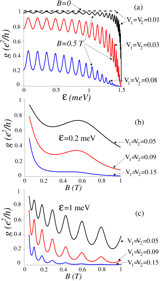
Figure 3: (Color online) Conductance [see, Eq. (22)] vs. (a) energy below the band gap $E_{g}=1.5$ meV and (b,c) vs. magnetic field. $V_{1,2}$ are in units of meV$\cdot\mu$m; $d_{12}=3\mu$m.

In contrast, in strong magnetic fields, scattering of the same strength is sufficient to suppress the conductance, $g$ near the band gap where the QSH-QH transition occurs [cf. dashed and solid curves for $V_{1,2}=0.01$ meV$\cdot\mu$m near $E_{g}=1.5$ meV in Fig. 3(a)]. Figs 3(a),(b) and (c) also show that the conductance suppression is accompanied by Fabry-Perot-type oscillations due to interference of the counter-propagating channels which acquire the energy- and field-dependent phase difference $(k_{+}-k_{-})d_{12}$, in scattering between the defects.

In our model the upper magnetic field limit lies in the range of a few Tesla. This estimate is based on Refs. König et al. (2008); Schmidt et al. (2009) predicting another ($B$-field induced) QSH-QH transition due to a quadratic correction ${\cal B}{\bf k}^{2}$ to the mass term in effective Hamiltonian (2). The smallness of the parameter ${\cal B}|M|/2\hbar^{2}\upsilon^{2}\ll 1$ König et al. (2008); Schmidt et al. (2009) allows us to neglect such ${\bf k}^{2}$ term and to meet, at the same time, the strong field condition $\hbar\upsilon/\lambda|M|>1$.

Conclusions.- We have studied the longitudinal conductance of helical spin edge channels in HgTe quantum wells in strong magnetic fields. As the Fermi level approaches the band gap, the conductance vanishes due to the combined effect of the spectral nonlinearity and channel backscattering. Such energy dependence indicates a transition between the quantum spin Hall and dissipationless quantum Hall regimes. The conductance exhibits $B^{-2N}$ magnetic field dependence, determined by the number $N$ of backscattering centers on the edge. This suggests a simple way to detect defects in ballistic QSH devices using standard magnetoresistance measurements.

Acknowledgements. We thank Shou-Cheng Zhang, Qiaoliang Qi, Joseph Maciejko, Alena Novik, Hartmut Buhmann, Laurens Molenkamp and Björn Trauzettel for enlightening discussions. The work was financially supported by the DFG Emmy-Noether Programme (G.T.) and by DFG grant HA5893/1-1 (G.T. and E.H.).

References

- Kane and Mele (2005) C. L. Kane and E. J. Mele, Phys. Rev. Lett. 95, 226801 (2005).
- Bernevig et al. (2006) B. A. Bernevig, T. L. Hughes, and S. C. Zhang, Science 314, 1757 (2006).
- Murakami (2006) S. Murakami, Phys. Rev. Lett. 97, 236805 (2006).
- König et al. (2007) M. König et al., Science 318, 766 (2007).
- König et al. (2008) M. König et al., J. Phys. Soc. Jpn. 77, 031007 (2008).
- Roth et al. (2009) A. Roth et al., Science 325, 294 (2009).
- Abanin et al. (2006) D. A. Abanin, P. A. Lee, and L. S. Levitov, Phys. Rev. Lett. 96, 176803 (2006).
- Abanin et al. (2007) D. A. Abanin et al., Phys. Rev. Lett. 98, 196806 (2007).
- Nomura and MacDonald (2006) K. Nomura and A. H. MacDonald, Phys. Rev. Lett. 96, 256602 (2006).
- Sheng et al. (2005) L. Sheng et al., Phys. Rev. Lett. 95, 136602 (2005).
- Shimshoni et al. (2009) E. Shimshoni, H. A. Fertig, and G. V. Pai, Phys. Rev. Lett. 102, 206408 (2009).
- (12) J. Maciejko, X.-L. Qi, and S.-C. Zhang, arXiv:0907.4515.
- Halperin (1982) B. I. Halperin, Phys. Rev. B 25, 2185 (1982).
- MacDonald and Streda (1984) A. H. MacDonald and P. Streda, Phys. Rev. B 29, 1616 (1984).
- Schmidt et al. (2009) M. J. Schmidt et al., Phys. Rev. B 79, 241306(R) (2009).
- Berry and Mondragon (1987) M. V. Berry and R. J. Mondragon, Proc. R. Soc. Lond. A 412, 53 (1987).
- Zhou et al. (2008) B. Zhou et al., Phys. Rev. Lett. 101, 246807 (2008).
- Abramowitz and Stegun (1964) M. Abramowitz and I. Stegun, Handbook of Mathematical Functions with Formulas, Graphs, and Mathematical Tables (National Bureau of Standards, 1964).
- Akhmerov et al. (2009) A. R. Akhmerov et al., Phys. Rev. B 80, 195320 (2009).
- Fisher and Lee (1981) D. S. Fisher and P. A. Lee, Phys. Rev. B 23, 6851 (1981).