Critical behavior and entanglement of the random transverse-field Ising model
between one and two dimensions

Abstract

We consider disordered ladders of the transverse-field Ising model and study their critical properties and entanglement entropy for varying width, $w\leq 20$, by numerical application of the strong disorder renormalization group method. We demonstrate that the critical properties of the ladders for any finite $w$ are controlled by the infinite disorder fixed point of the random chain and the correction to scaling exponents contain information about the two-dimensional model. We calculate sample dependent pseudo-critical points and study the shift of the mean values as well as scaling of the width of the distributions and show that both are characterized by the same exponent, $\nu(2d)$. We also study scaling of the critical magnetization, investigate critical dynamical scaling as well as the behavior of the critical entanglement entropy. Analyzing the $w$-dependence of the results we have obtained accurate estimates for the critical exponents of the two-dimensional model: $\nu(2d)=1.25(3)$, $x(2d)=0.996(10)$ and $\psi(2d)=0.51(2)$.

I Introduction

In nature there are materials, which are in a way between two integer dimensions, such as they are built from $(d-1)$-dimensional layers having a finite width, $w$. Examples are thin filmsthinfilms , magnetic multilayersmajkrzak91 or ladders of quantum spinsdagotto96 . One interesting question for such multilayer systems is the properties of critical fluctuations, when the linear extent of the layers, $L$, goes to infinity. If the system is classical having thermal fluctuations, finite-size scaling theoryfisherme ; barber can be applied. One basic observation of this theory is that for any finite $w$ the critical behavior is controlled by the fixed point of the $(d-1)$-dimensional system, but the scaling functions in terms of the variable, $w/L$, involve also the critical exponents of the $d$-dimensional system. For example the critical points, $T_{c}(w)$, measured at a finite width, $w$, approach the true $d$-dimensional critical point, $T_{c}\equiv T_{c}(\infty)$, as

$$T_{c}-T_{c}(w)\sim w^{-1/\nu_{s}}\;,$$ (1)

where the shift exponent, $\nu_{s}$, generally corresponds to the correlation-length exponent, $\nu$, in the $d$-dimensional system.

In a quantum system having a quantum critical point at zero temperature, $T=0$, by varying a control parameter, $\theta$, the dimensional cross-over is a more subtle problem. If the $d$-dimensional critical quantum system is isomorphic with a $(d+1)$-dimensional classical systemkogut , then results of finite-size scaling can be transferred to the quantum system, too. This is the case, e.g. for the quantum critical point of the $d$-dimensional transverse-field Ising model, which is equivalent to the critical point of the classical $(d+1)$-dimensional Ising model. However, the situation is more complicated for antiferromagnetic models with continuous symmetry, such as for Heisenberg antiferromagnetic spin ladders. In this case the form of low-energy excitations could sensitively depend on the value of $w$: if the ladder contains even number of legs there is a gap, whereas for odd number of legs the system is gaplessdagotto96 . In the following for quantum systems we restrict ourselves to models with a discrete symmetry, such as to the transverse-field Ising model.

In disordered systems, in which besides deterministic (thermal or quantum) fluctuations there are also disorder fluctuations in a sample of finite width one can define and measure a sample-dependent pseudo-critical point, $T_{c}(w)$ (or $\theta_{c}(w)$), and study its distributiondomany . In particular one concerns the shift of the mean value, $\overline{T_{c}}(w)$, and the scaling of the width of the distribution, $\Delta T_{c}(w)$. In this case besides the shift exponent, $\nu_{s}$, which is defined analogously to Eq.(1) one should determine the width exponent, $\nu_{w}$, too, which is defined by the scaling relation:

$$\Delta T_{c}(w)\sim w^{-1/\nu_{w}}\;.$$ (2)

According to renormalization group theoryaharony the finite-size scaling behavior of random classical systems depends on the relevance or irrelevance of the disorderharris . If the disorder represents an irrelevant perturbation at the pure system’s fixed point, which happens if the correlation length exponent in the pure system satisfies $\nu_{p}>2/d$, than for the disordered system we have $\nu_{s}=\nu_{p}$ and $\nu_{w}=2/d$ and the thermodynamic quantities at the fixed point are self-averaging. On the contrary for relevant disorder, which happens for $\nu_{p}<2/d$, there is a new conventional random fixed point with a correlation-length exponent, $\nu\geq 2/d$ccfs , and we have $\nu_{s}=\nu_{w}=\nu$. In this fixed point there is a lack of self-averaging. These predictions, which have been debated for some timepsz , were checked later for various modelsdomany ; aharony ; paz2 ; mai04 ; PS2005 .

For quantum systems quenched disorder is perfectly correlated in the (imaginary) time direction, therefore generally it has a more profound effect at a quantum critical pointqsg . In some cases the critical properties of the random model are controlled by a so called infinite disorder fixed pointfisher , in which the disorder fluctuations play a completely dominant rǒle over quantum fluctuations. This happens, among others for the random transverse-field Ising model, as shown by analytical resultsfisher in $1d$ and numerical resultspich98 ; motrunich00 ; lin00 ; karevski01 in $2d$. Finite-size scaling has been tested for the $1d$ model and a new scenario is observedilrm . The finite-size transition points, denoted by $\theta_{c}(L)$ in a system of length, $L$, are shown to be characterized by two different exponents, $\nu_{s}<\nu_{w}$. This means, that asymptotically $\Delta\theta_{c}(L)/[\overline{\theta_{c}}(\infty)-\overline{\theta_{c}}(L)]\to\infty$, which is just the opposite limit as known for irrelevant disorder.

In the present paper we go to the two-dimensional problem and study the finite-size scaling properties of ladders of random transverse-field Ising models. For this investigations we use a numerical implementation of the so called strong disorder renormalization group methodim . As in $2d$ this method is expected to be asymptotically exact in large scales. In the numerical implementation of the method we have used efficient computer algorithms and in this way we could treat ladders with a large number of sites: we went up to lengths $L=4096$ for $w=20$ legs and used $4\times 10^{4}$ random samples. Our aim with these investigations is threefold. First, we want to clarify the form of finite-size scaling valid for this random quantum model. Second, using the appropriate form of the scaling Ansatz we want to calculate estimates for the critical exponents of the 2d model. Previous studiespich98 ; motrunich00 ; lin00 ; karevski01 ; vojta09 in this respect have quite large error bars and we want to increase the accuracy of the estimates considerably. Our third aim is to calculate also the entanglement entropyAmicoetal08 in the ladder geometry and study its cross-over behavior between onerefael and two dimensionslin07 ; yu07 .

The structure of the rest of the paper is the following. The model and the method of the calculation is presented in Sec. II. In Sec. III finite-size transition points are calculated and their distribution (shift and width) is analyzed. In Sec. IV we present calculations at the critical point about the magnetization and the dynamical scaling behavior. Results about the entanglement entropy are presented in Sec.V. Our paper is closed by a discussion.

II Model and method

II.1 Random transverse-field Ising ladder

We consider the random transverse-field Ising model in a ladder geometry in which the sites, $i$ and $j$, are taken from a strip of the square lattice of length, $L$, and width, $w$. We use periodic boundary conditions in both directions. The model is defined by the Hamiltonian:

$${\cal H}=-\sum_{\langle ij\rangle}J_{ij}\sigma_{i}^{x}\sigma_{j}^{x}-\sum_{i}h_{i}\sigma_{i}^{z}$$ (3)

in terms of the Pauli-matrices, $\sigma_{i}^{x,z}$. Here the first sum runs over nearest neighbor sites and the $J_{ij}$ couplings and the $h_{i}$ transverse fields are independent random numbers, which are taken from the distributions, $p(J)$ and $q(h)$, respectively. For concreteness we use box-like distributions: $p(J)=1$, for $0\leq J\leq 1$ and $p(J)=0$, for $J>1$; $q(h)=1/h_{0}$, for $0\leq h\leq h_{0}$ and $q(h)=0$, for $h>h_{0}$. We consider the system at $T=0$ and use $\theta=\ln h_{0}$ as the quantum control parameter.

In the thermodynamic limit, $L\to\infty$, the system in Eq.(3) displays a paramagnetic phase, for $\theta>\theta_{c}(w)$, and a ferromagnetic phase, for $\theta<\theta_{c}(w)$. In between there is a random quantum critical point at $\theta=\theta_{c}(w)$ and we are going to study its properties for various widths, $w$.

II.2 Strong disorder renormalization group method

The model is studied by the strong disorder renormalization group methodim , which has been introduced by Ma, Dasgupta and Humdh and later developed by D. Fisherfisher and others. In this method the largest local term in the Hamiltonian (either a coupling or a transverse field) is successively eliminated and at the same time new terms are generated between remaining sites. If the largest term is a coupling, say $J_{2,3}=\Omega$ connecting sites $2$ and $3$, ($\Omega$ being the energy-scale at the given RG step), then after renormalization the two sites form a spin cluster with an effective moment $\tilde{\mu}_{2,3}=\mu_{2}+\mu_{3}$, where in the starting situation each spin has unit moment, $\mu_{i}=1$. The spin cluster is put in an effective transverse field of strength: $\tilde{h}_{2,3}\approx h_{2}h_{3}/J_{2,3}$, which is obtained in second order perturbation calculation. On the other hand, if the largest local term is a transverse-field, say $h_{2}=\Omega$, then site $2$ is eliminated and new couplings are generated between each pairs of spins, which are nearest neighbors to $2$. If say $k$ and $l$ are nearest neighbor spins to $2$, than the new coupling connecting them is given by: $\tilde{J}_{k,l}\approx J_{2,k}J_{2,l}/h_{2}$, also in second order perturbation calculation. If the sites $k$ and $l$ are already connected by a coupling, $J_{k,l}\neq 0$, than for the renormalized coupling we take $max[J_{k,l},\tilde{J}_{k,l}]$. This last step is justified if the renormalized couplings have a very broad distribution, which is indeed the case at infinite disorder fixed points. The renormalization is repeated: at each step one more site is eliminated and the energy scale is continuously lowered. For a finite system the renormalization is stopped at the last site, where we keep the energy-scale, $\Omega^{*}$, and the total moment, $\mu^{*}$, as well as the structure of the clusters.

II.3 Known exact results in the chain geometry

The renormalization has special characters in the chain geometry, i.e. with $w=1$. In this case the topology of the system stays invariant under renormalization and the couplings and the transverse fields are dual variables. From this follows that at the quantum critical point the couplings and the transverse fields are decimated symmetrically, thus the critical point is located at $\theta_{c}(1)=0$pfeuty . The RG equations for the distribution function of the couplings and that of the transverse fields can be written in closed form as an integro-differential equation, which has been solved analytically both at the critical pointfisher and in the off-critical region, in the so-called Griffiths-phasei02 . Here we list the main results.

The energy-scale, $\Omega$, and the length-scale, $L$, are related as:

$$\ln(\Omega_{0}/\Omega)\sim L^{\psi}\;,$$ (4)

with an exponent: $\psi(1d)=1/2$. (Here $L$ can be the size of a finite system and $\Omega_{0}$ is a reference energy scale.) The average spin-spin correlation function is defined as $G(r)=[\langle\sigma_{i}^{x}\sigma_{i+r}^{x}\rangle]_{\rm av}$, where $\langle\dots\rangle$ denotes the ground-state average and $[\dots]_{\rm av}$ stands for the averaging over quenched disorder. In the vicinity of the critical point $G(r)$ has an exponential decay:

$$G(r)\sim\exp(-r/\xi)\;,$$ (5)

in which the correlation length, $\xi$, is divergent at the critical point as:

$$\xi\sim|\theta-\theta_{c}|^{-\nu}\;,$$ (6)

with $\nu(1d)=2$. At the critical point the average correlations have a power-law decay:

$$G(r)\sim r^{-2x},\quad\theta=\theta_{c}\;,$$ (7)

with a decay exponent:

$$x(1d)=(3-\sqrt{5})/4\;.$$ (8)

The average cluster moment, $\mu$, is related to the energy-scale, $\Omega$ as:

$$\mu\sim[\ln(\Omega_{0}/\Omega)]^{\phi}\;,$$ (9)

with $\phi(1d)=(1+\sqrt{5})/2$. The average cluster moment can be expressed also with the size as $\mu\sim L^{d_{f}}$, where the fractal dimension of the cluster is expressed by the other exponents as:

$$d_{f}=\phi\psi=d-x\;,$$ (10)

with $d=1$.

III Finite-size critical points

III.1 Results in the chain geometry

In the chain geometry finite-size critical points are studied in Ref.ilrm , in which they are located by different methods, which all are based on the free-fermion mapping of the problemlsm . The finite-size critical points are shown to satisfy the micro-canonical condition:

$$\sum_{i=1}^{L}\ln J_{i}=\sum_{i=1}^{L}\ln h_{i}\;,$$ (11)

from which follows that the distribution of $\theta_{c}(L)$ is Gaussian with zero mean and with a mean deviation of $\Delta\theta_{c}(L)\sim L^{-1/2}$. Consequently the width-exponent of the distribution is given by:

$$\nu_{w}=\nu(1d)=2\;.$$ (12)

On the other hand the shift-exponent is given by:

$$\nu_{s}=1\;,$$ (13)

although in some cases (c.f. for periodic boundary conditions) the prefactor of the scaling function can be vanishing.

III.2 The doubling method

In the ladder geometry, i.e. for $w\geq 2$, the free-fermionic mapping is no longer valid, therefore new methods have to be utilized to locate pseudo-critical points. Here we used the doubling method combined with the strong disorder renormalization group.

In the doubling procedurePS2005 for a given random sample ($\alpha$) of length $L$ and width $w$, we construct a replicated sample ($2\alpha$) of length $2L$ and width $w$ by gluing two copies of ($\alpha$) together and study the ratio of the magnetizations: $r_{m}(\alpha,L,w)=m(2\alpha,2L,w)/m(\alpha,L,w)$, which are calculated by the strong disorder renormalization group method. In Fig.1 we illustrate the $\theta$ dependence of the total magnetic moments, $\mu(2\alpha,2L,w)$ and $\mu(\alpha,L,w)$, for a given sample of a $w=2$-leg $L=128$ ladder. The corresponding ratio of the magnetizations, $r_{m}(\alpha,L,w)$, is shown in the upper inset of this figure. It is seen, that in the ordered phase: $\theta<\theta_{c}(\alpha,L,w)$ this ratio approaches $r_{m}(\alpha,L,w)\to 1$. On the other hand in the disordered phase: $\theta>\theta_{c}(\alpha,L,w)$ the magnetizations approach their minimal values, which in the SDRG method can be $1/2L$ and $1/L$, respectively, thus we have $r_{m}(\alpha,L,w)\to 1/2$. In between there is a sudden change in the value of this ratio, which can be used to define a sample-dependent pseudo-critical point, $\theta_{c}(\alpha,L,w)$.

There is another possibility, if we consider the ratio of the two gaps: $r_{\Omega}(\alpha,L,w)=\Omega(2\alpha,2L,w)/\Omega(\alpha,L,w)$, which are also calculated by the strong disorder renormalization group method. In Fig.1 we show the two log-gaps, $-\log\Omega(2\alpha,2L,w)$ and $-\log\Omega(\alpha,L,w)$, for the same sample as before and the corresponding ratio, $r_{\Omega}(\alpha,L,w)$, is put in the upper inset of this figure. It is seen that this ratio in the ordered phase, $\theta<\theta_{c}(\alpha,L,w)$, approaches $r_{\Omega}(\alpha,L,w)\to 0$ and in the disordered phase: $\theta>\theta_{c}(\alpha,L,w)$, goes to $r_{\Omega}(\alpha,L,w)\to 1$. In between this ratio has a quick variation and we can fix the point where $r_{\Omega}(\alpha,L,w)=1/2$ to define a sample-dependent pseudo-critical point, $\theta_{c}(\alpha,L,w)$.

III.3 Numerical results

III.3.1 Comparison of the two definitions

In the doubling method we have calculated pseudo-critical points by using both ratios. We have observed, that for a given sample $\theta_{c}^{(\Omega)}$ calculated from the ratio of the gaps is always somewhat smaller, than $\theta_{c}^{(m)}$, which is obtained from the ratio of the magnetizations. This is illustrated in the upper inset of Fig.1 for a given sample. We have also calculated for several realizations the ratio of the two pseudo-critical points, $\theta_{c}^{(\Omega)}/\theta_{c}^{(m)}$, which is shown in the lower inset of Fig.1 as a function of $\theta_{c}^{(m)}$ for the $w=10$ leg ladder for various lengths, $L=32,64$ and $128$. The relative difference between the two pseudo-critical points is indeed vary small, it is of the order of $10^{-3}$ and this is decreasing with increasing $L$ and $w$. In the following we restrict ourselves to those pseudo-critical points, which are calculated from the ratio of the magnetization and which have a relative precision of $10^{-4}$ for each sample.

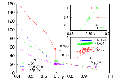
Figure 1: (Color online) SDRG results for the total magnetic moments, $\mu(2\alpha)$ and $\mu(\alpha)$, as well as for the log-gaps, $-\log\Omega(2\alpha)$ and $-\log\Omega(\alpha)$, as a function of the control parameter, $\theta$, for a given realization ($\alpha$) of a $w=2$-leg $L=128$ ladder and its double ($2\alpha$), see text. Upper inset: ratio of the magnetizations, $r_{m}$, and that of the gaps, $r_{\Omega}$, as a function of $\theta$ (log-lin scale) in the vicinity of the finite-size transition points. The finite-size critical point for $r_{m}$ is given at the jump, for $r_{\Omega}$ it is located where $r_{\Omega}=1/2$. Lower inset: Ratio of the two pseudo-critical points, $\eta=\theta_{c}^{(\Omega)}/\theta_{c}^{(m)}$ as a function of $\theta_{c}^{(m)}$ for the $w=10$ leg ladder for various lengths and for 500 realizations.

III.3.2 Distribution of finite-size critical points

We have calculated the distribution of pseudo-critical points for ladders with a fixed number of legs, $1\leq w\leq 20$, for varying lengths, $L=2^{l}$, with $l=5,6,\dots,10$. Indeed, for the largest values of $L$ the relation, $w/L\ll 1$ is well satisfied. For the $w=10$ leg ladder the distribution of the $\theta_{c}$ values for various lengths are shown in Fig.2, which are obtained for $10^{4}$ realizations for each cases. As seen in this figure the width of the distribution is decreasing with increasing $L$ and there is only a weak shift of the position of the maximum. The distributions somewhat deviate from Gaussians, they are asymmetric, as can be seen in the log-lin plot in the inset of Fig.2. With increasing $L$, however, the skewness of the distribution is decreasing, which is in agreement with the expectation, that in the $w/L\to 0$ limit we get back the corresponding results for chains.

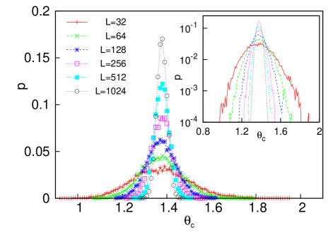
Figure 2: (Color online) Distribution of the pseudo-critical points, $\theta_{c}$, for the $w=10$ leg ladder for various lengths and for $10^{4}$ realizations. In the inset in a log-lin plot deviations from the Gaussian distributions are seen, which however are decreasing with increasing $L$.

III.3.3 ”True” critical points for ladders

For a fixed value of the number of legs, $w$, we have calculated the mean value of the pseudo-critical points. We have observed that the $L$-dependence of $\overline{\theta_{c}}(w,L)$ becomes weaker and weaker with increasing $L$, which is in agreement with the fact, that the system approaches more and more the chain geometry. Due to this one can obtain accurate estimates in the thermodynamic limit for the ”true” critical points of ladders, which are listed in Table 1 for different number of legs. Here the errors are merely due to disorder fluctuations since for $L\geq 192$ the finite length effects are negligible.

Table 1: Quantum critical points of ladders of the random transverse-field Ising model, $\theta_{c}$, and the asymptotic prefactor of the standard deviation in Eq.(17), $a$, for different number of legs.

$w$	$\theta_{c}$	$a$	$w$	$\theta_{c}$	$a$
$1$	$0.00021(30)$	$1.413(8)$	$11$	$1.39399(20)$	$0.728(5)$
$2$	$0.64418(15)$	$0.997(1)$	$12$	$1.41211(10)$	$0.709(3)$
$3$	$0.94736(10)$	$0.925(5)$	$13$	$1.42778(10)$	$0.696(2)$
$4$	$1.08059(15)$	$0.881(2)$	$14$	$1.44165(20)$	$0.681(4)$
$5$	$1.16859(10)$	$0.844(5)$	$15$	$1.45397(10)$	$0.669(4)$
$6$	$1.23207(15)$	$0.815(5)$	$16$	$1.46472(15)$	$0.658(4)$
$7$	$1.27962(15)$	$0.807(4)$	$17$	$1.47445(10)$	$0.650(4)$
$8$	$1.31727(20)$	$0.781(3)$	$18$	$1.48332(10)$	$0.640(1)$
$9$	$1.34787(10)$	$0.763(3)$	$19$	$1.49095(30)$	$0.626(4)$
$10$	$1.37270(15)$	$0.733(2)$	$20$	$1.49855(15)$	$0.620(2)$

Here we also list our estimate for the chain, $w=1$, which agrees within the error of the calculation with the exact result: $\theta_{c}(1)=0$ and $a(1)=\sqrt{2}$ (see Sec.III.3.4).

Figure 3: (Color online) Critical points of the ladders for varying number of legs, $w$, and the extrapolation curve (broken (green) line) for large $w$. Upper inset: estimates of the inverse of the local shift exponent, $1/\nu_{s}(w)$, calculated through Eq.(14). The broken (green) straight line indicates the extrapolation through $1/w$. Lower inset: ratio of the scaled difference of the critical points and the scaled standard deviations as a function of $1/w$(see text). The horizontal broken (green) line at $rs=1.$ indicates a value which is close to the expected asymptotic behavior.

These data approach the critical point in the 2d system, $\theta_{c}(2d)$, see Fig.3. Here the corrections for large-$w$ are expected to have a power-law form, and analogously to Eq.(1), it contains the shift exponent, $\nu_{s}$, of the 2d system.

Estimates for the effective ($w$-dependent) values of the shift exponent are obtained from the ratio of the second and the first finite differences:

$$\frac{1}{\nu_{s}(w)}=\frac{\Delta_{2}\theta_{c}(w)}{\Delta_{1}\theta_{c}(w)}w-1\;,$$ (14)

which are calculated at the central point of five-point fits. The effective exponents are given in the upper inset of Fig.3, which are extrapolated as $1/\nu_{s}(2d)=0.81(10)$, thus we obtain:

$$\nu_{s}(2d)=1.24(15)\;.$$ (15)

III.3.4 Scaling of the width of the distribution

We have measured the standard deviation of the distribution of the pseudo-critical points, $\Delta\theta_{c}(w,L)$, for ladders with $w$ legs and with a varying length, $L$. This quantity is expected to scale with the length as:

$$\Delta\theta_{c}(w,L)=L^{-1/\nu_{w}(2d)}\sigma(w/L)\;,$$ (16)

where the scaling function, $\sigma(y)$, behaves for small arguments as: $\sigma(y)\sim y^{-1/\nu_{w}(2d)+1/\nu_{w}(1d)}$. From this follows, that for finite widths we have:

$$\Delta\theta_{c}(w,L)=L^{-1/\nu_{w}(1d)}a(w)\;,$$ (17)

with a prefactor, $a(w)$, which behaves for large $w$ as $a(w)\sim w^{\epsilon}$, with an exponent $\epsilon=-1/\nu_{w}(2d)+1/\nu_{w}(1d)$. We have checked this scenario by analyzing the data for $\Delta\theta_{c}(w,L)$. First, for a fixed $w$ we have fitted a function $a(w)L^{-\omega}$, with a free parameter, $\omega$. We have found that for each widths, $1\leq w\leq 20$, the exponent $\omega$ agrees with $1/\nu_{w}(1d)=0.5$, within a few thousands of error, as illustrated in Fig.4.

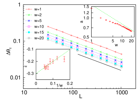
Figure 4: (Color online) Scaling of the width of the distribution of the pseudo-critical points, $\Delta\theta_{c}(w,L)$, with $L$ for different number of legs, $w$. In a log-log plot the slope of the curves are compatible with the theoretical prediction, $\nu_{w}(1d)=1/2$, which is indicated by a full straight line. In the upper inset the limiting value of the prefactor, $a(w)$ is shown as a function of $w$ in a log-log plot. The dashed (green) straight line has a slope, $\epsilon=0.30$, as extrapolated from effective exponents in the lower inset.

In the next step we have fixed the value of $\omega=0.5$ and estimated the limiting value of $\Delta\theta_{c}(w,L)L^{0.5}$ for large $L$, which is denoted by $a(w)$. These limiting values are presented in Table 1, which are analyzed for large $w$. As seen in the upper inset of Fig. 4 in a log-log plot the $a(w)$ values are asymptotically on a straight line. We have calculated effective, $w$-dependent exponents: $\epsilon(w)=\log(a(w)/a(w/2))/\log 2$, which are presented in the lower inset of Fig.4 as a function of $1/w$. These effective exponents have a weak $w$-dependence and we estimate its limiting value as $\epsilon=-0.30(2)$. With this we have for the width exponent in $2d$:

$$\nu_{w}(2d)=1.25(3)\;.$$ (18)

Closing this section we try to decide in a direct way about the relation between the two exponents, $\nu_{s}(2d)$ and $\nu_{w}(2d)$. For this we form the scaled difference: $d\theta_{c}(w)=\Delta_{1}\theta_{c}(w)w$ (see Eq.(14)), which scales as $w^{-1/\nu_{s}}$, as well as the scaled standard deviation: $sa(w)=w^{-0.5}a(w)$, which scales as $w^{-1/\nu_{w}}$, and form their ratio, $rs(w)=d\theta_{c}(w)/sa(w)$. As seen in the lower inset of Fig.3 this ratio approaches a finite value which can be estimated as $rs=1.01(2)$. Thus we can conclude that at the infinite disorder fixed point of the $2d$ random transverse-field Ising model the shift and the width exponents are equal and they correspond to the correlation length exponent of the model.

Using the best estimate for $\nu_{s}(2d)=\nu_{w}(2d)$ and including the first analytic correction to scaling term: $\theta_{c}=\theta_{c}(w)-Aw^{-1/\nu_{s}}(1+B/w)$ we fit our data (see Fig.3) and obtain for the critical point of the $2d$ system:

$$\theta_{c}(2d)=1.676(5)\;.$$ (19)

This value is in agreement with the previous estimate, $\theta_{c}(2d)=1.680(5)$, in Ref.[yu07, ].

IV Scaling at the critical point

Having estimates for the critical points of random ladders with $w$ legs, $\theta_{c}(w)$, we have calculated scaling of the magnetization at the critical point as well as the critical dynamical scaling. These calculations are made for lengths up to $2^{12}$ and for $4\times 10^{4}$ realizations.

IV.1 Magnetization

We have calculated the average total magnetic moment at the critical point, $\mu_{c}(w,L)$, for varying lengths, $L$, which is expected to scale as:

$$\mu_{c}(w,L)=L^{d_{f}(2d)}\tilde{\mu}_{c}(w/L)\;,$$ (20)

with a scaling function, which behaves for small arguments as: $\tilde{\mu}_{c}(y)\sim y^{d_{f}(2d)-d_{f}(1d)}$. Then, for a finite width, $w$, we have:

$$\mu_{c}(w,L)=L^{d_{f}(1d)}b(w)\;,$$ (21)

with a prefactor, which for large $w$ behaves as: $b(w)\sim w^{\kappa}$, with $\kappa=d_{f}(2d)-d_{f}(1d)$.

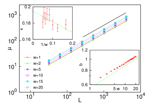
Figure 5: (Color online) Scaling of the average total magnetic moment at the critical point of a ladder with $w$ legs and length $L$, $\mu_{c}(w,L)$. In the log-log plot the slope of the curves are compatible with the theoretical prediction, $d_{f}(1d)$ in Eq.(10), which is indicated by a full straight line. In the lower inset the limiting value of the prefactor, $b(w)$ is shown as a function of $w$ in a log-log plot. The dashed (green) straight line has a slope, $\kappa=0.195$, as extrapolated from effective exponents in the upper inset.

The scaling Ansatz in Eq.(21) is checked in Fig.5. Then, we have calculated the limiting value of $L^{-d_{f}(1d)}\mu_{c}(w,L)$, which is denoted by $b(w)$ and which is presented as a function of $w$ in a log-log plot in the lower inset of Fig.5. Effective, $w$-dependent exponents are calculated, which are extrapolated in the upper inset of Fig.5 giving $\kappa=0.195(10)$. Thus the fractal dimension in $2d$ is $d_{f}(2d)=d_{f}(1d)+\kappa$ and from Eq.(10) we obtain for the magnetization scaling dimension:

$$x(2d)=0.996(10)\;.$$ (22)

IV.2 Dynamical scaling

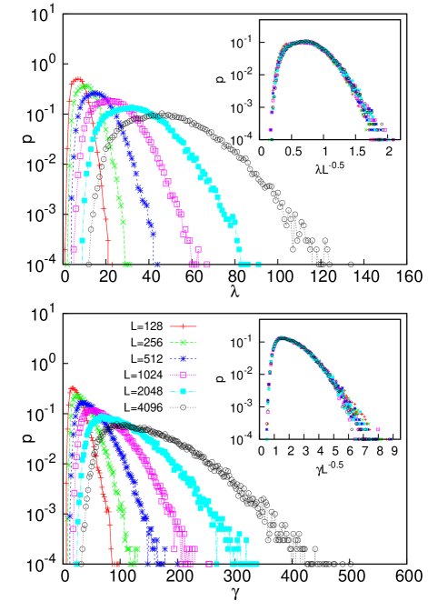
Figure 6: (Color online) Distribution of the last decimated log-coupling, $\lambda$, (upper panel) and the last decimated log-transverse field, $\gamma$ (lower panel) for various lengths, $L$, for the $w=10$-leg ladder. In the insets the distribution of the scaled variables: $\lambda L^{-0.5}$ and $\gamma L^{-0.5}$, respectively are shown.

At an infinite disorder fixed point there is a special form of dynamical scaling, as given in Eq.(4). The energy scale of a sample at the end of the renormalization can be defined either by the value of the last decimated (log) coupling $-\log\tilde{J}=\lambda$ or by the last decimated (log) transverse field $-\log\tilde{h}=\gamma$. The distribution of $\lambda$ as well as $\gamma$ are shown in Fig.6 in upper and in the lower panel, respectively, for the $w=10$-leg ladder for various values of the length, $L$. An appropriate scaling collapse of the date is observed in terms of the scaling variables, $\lambda L^{-\psi}$ and $\gamma L^{-\psi}$, with $\psi=\psi(1d)=1/2$, as illustrated in the insets.

In order to have a more quantitative picture about dynamical scaling we consider the mean value: $\Gamma(w,L)=[\gamma(w,L)]_{\rm av}$ and the standard deviation, $\Delta\Gamma(w,L)$ and similarly, $\Lambda(w,L)=[\lambda(w,L)]_{\rm av}$ and $\Delta\Lambda(w,L)$. All these quantities are expected to scale in the same way, for example with $\Gamma(w,L)$ we have:

$$\Gamma(w,L)=L^{\psi(2d)}\tilde{\Gamma}(w/L)\;,$$ (23)

with $\tilde{\Gamma}(y)\sim y^{\psi(2d)-\psi(1d)}$. For a finite width, $w$, we have then:

$$\Gamma(w,L)=L^{\psi(1d)}g(w)\;,$$ (24)

with $g(w)\sim w^{\delta}$ for large $w$ with $\delta=\psi(2d)-\psi(1d)$.

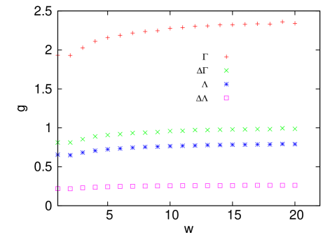
Figure 7: (Color online) Scaling functions for typical energy-scales: $g(w)=\lim_{L\to\infty}G(w,L)L^{-1/2}$, in which $G(w,L)$ is either $\Gamma(w,L)$, $\Delta\Gamma(w,L)$, $\Lambda(w,L)$ or $\Delta\Lambda(w,L)$, see text.

We have checked that the scaling form in Eq.(24) is indeed satisfied for all values of $1\leq w\leq 20$ and than calculated the limiting value of $\Gamma(w,L)L^{-1/2}$, which is denoted by $g(w)$. As illustrated in Fig.7 the scaling functions of the typical energy-scales have only a very weak $w$ dependence, and we estimate (not shown) a small exponent: $\delta=0.01(2)$. Thus we have for the $\psi$ exponent in the $2d$ model:

$$\psi(2d)=0.51(2)\;.$$ (25)

V Entanglement entropy

In the ladder geometry we consider a block, $\cal{A}$, which contains all the $w$ legs and has a length, $\ell\ll L$. Consequently the block has two parallel lines of width, $w$, at which it has contact with the rest of the system, $\cal{B}$. The entanglement of $\cal{A}$ with $\cal{B}$ is quantified by the von-Neumann entropyAmicoetal08 :

$${\cal S}_{\cal A}(w,\ell)=-{\rm Tr}_{\cal A}(\rho_{\cal A}\log\rho_{\cal A})\;,$$ (26)

in terms of the reduced density matrix: $\rho_{\cal A}=Tr_{{\cal B}}|\Psi\rangle\langle\Psi|$, where $|\Psi\rangle$ denotes a pure state (in our case the ground state) of the complete system.

At the critical point of a random quantum system the properties of which are controlled by an infinite disorder fixed point the asymptotic behavior of the entropy in the large $l$ limit can be obtained by the strong disorder renormalization group method. For the random transverse-field Ising model entanglement between $\cal{A}$ and $\cal{B}$ are given by such renormalized spin clusters, which contain sites both in $\cal{A}$ and in $\cal{B}$, and the cluster is eliminated at some point of the renormalizationrefael ; lin07 ; yu07 . Due to the very broad distribution of the effective couplings and transverse fields, the cluster at the energy scale of its decimation is in a so called GHZ entangled state of the form: $1/\sqrt{2}(|\uparrow\uparrow\dots\uparrow\rangle+|\downarrow\downarrow\dots\downarrow\rangle)$. Each such cluster contribute by an amount of $\log 2$ to the entanglement entropy, thus calculation of the entropy is equivalent to a cluster counting problem, which is illustrated in Fig.8.

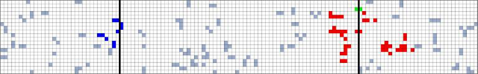
Figure 8: (Color online) Structure of the decimated spin clusters at the critical point of a ladder of $20\times 128$ sites, which is devided into two equal blocks the boundary of which is indicated by thick vertical lines. There are three clusters, denoted by blue, red and green colors, respectively, which contain sites at both blocks and thus result in an entropy $3\times\log 2$.

In the chain geometry the asymptotic behavior of the entropy at the critical point is obtained from the analytical solution of the RG equations asrefael :

$${\cal S}_{\cal A}(1,\ell)\approx\frac{c(1)}{3}\log\ell+k(1)\;,$$ (27)

where $k(1)$ is a non-universal constant, which depends on the form of the disorder, whereas the prefactor of the logarithm, $c(1)$, which is also called as the effective central charge, is universal and given by: $c(1)=\ln 2/2$. This result is checked numerically in Ref.[il08, ]. In the two-dimensional case, which is expected to hold for $w/L=O(1)$, there are somewhat conflicting numerical results at the critical point. Lin et al.lin07 have observed a double-logarithmic multiplicative factor to the area-law: ${\cal S}_{\cal A}(\ell,\ell)\approx\ell\log\log\ell$ whereas later Yu et al.yu07 argued to have only a subleading logarithmic term to the area law: ${\cal S}_{\cal A}(\ell,\ell)\approx a\ell+b\log\ell+k$.

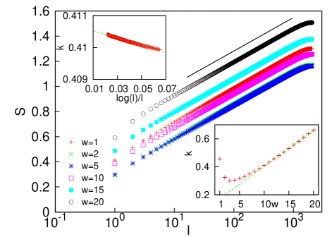
Figure 9: (Color online) The log-$\ell$-dependence of the entanglement entropy at the critical point of ladders for different number of legs, $w$, and for $L=4096$. The linear part of the curves has approximately the same slope, which is consistent with $\ln 2/6$, as indicated by a full straight line. Upper inset: the non-universal part of the critical entropy, $k(w,\ell)$, for the $w=10$-leg ladder and its extrapolation for $\ell\gg w$ (but $\ell\ll L=4096$) with a correction term of $\sim\log\ell/\ell$. Lower inset: the asymptotic value of the non-universal part of the critical entropy, $k(w)$, as a function of $w$. Asymptotically there is a linear $w$-dependence, which is shown by a broken (green) straight line.

Here we study numerically the critical ladder systems with various number of legs and try to identify the cross-over between one- and two dimensions. To illustrate the $\ell$ dependence of the entanglement entropy in Fig.9 we show ${\cal S}_{\cal A}$ as a function of $\log\ell$ for different number of legs for $L=4096$. (We have checked, that the asymptotic results does not change for $L=2048$.) The central parts of the curves are very well linear having approximately the same slope, which is consistent with the exact result for the $w=1$ chain geometry. Thus we conclude that the effective central charge, $c(w)$, does not depend on the number of legs.

In the next step we fix $c(w)=\ln 2/2$, calculate the non-universal term: $k(w,\ell)={\cal S}_{\cal A}(w,\ell)-\frac{\ln 2}{6}\log\ell$ and take its limit, $k(w)$, for large $\ell$ (but still with $\ell\ll L$). As illustrated in the upper inset of Fig.9 the $\ell$-dependent correction term is approximated as $\log\ell/\ell$ and the asymptotic non-universal terms, $k(w)$, are shown for different number of legs in the lower inset of Fig.9. One can see that starting with the chain, $w=1$, first $k(w)$ is decreasing, has a minimum around $w=3$ and then starts to increase. This increase for large $w$ is approximately linear, we have fitted: $k(w)=0.0256(5)w+0.148(5)$. This linear increase is compatible with the area law, which should hold for non-critical systems and for large blocks. Our analysis can be used to clarify the one- to two-dimensional cross-over of the entropy in the limit $w/\ell\ll 1$. However, our data can not be used to make predictions further, for $w/L=O(1)$, i.e. for the two-dimensional case. For this one should analyze the occurrent and possibly very weak $w$ dependence of the prefactor of the linear term of $k(w)$, which however can not be done with our data, which are only up to $w=20$.

VI Discussion

In this paper we have studied the critical properties and the entanglement entropy of random transverse-field Ising models in the ladder geometry by the strong disorder renormalization group method. In our numerical calculation we went up to w=20 legs and with a length up to L=4096 for $4\times 10^{4}$ realizations. In principle the sizes of the systems could have been increased further, but it was not necessary. With $L$ we have already reached the limit where no further systematic finite-size effects are seen. On the other hand for larger values of $w$ we would have obtained too large errors in calculating quantities, such as through two-point fit.

First, we have calculated sample dependent finite-size critical points, which are obtained by the doubling procedure and the strong disorder renormalization group method. We have analyzed the shift of the mean value of the transition points and the width of the distribution as a function of the number of legs, $w$, and estimated the exponents of the $2d$ model, $\nu_{s}(2d)$ and $\nu_{w}(2d)$, respectively. These are found to be identical and given by the correlation-length exponent of the $2d$ model. Consequently the scaling behavior of the pseudo-critical points of the $2d$ random transverse-field Ising model is in the same form as for classical and conventional random fixed pointsaharony . In this respect there is a difference with the $1d$ modelilrm , in which $\nu_{s}(1d)<\nu_{w}(1d)$. For this latter model probably the free-fermionic character could be the reason for the different scaling properties. Our estimate for the correlation length exponent, $\nu(2d)=1.25(3)$, is clearly larger than the possible limiting value of $2/d$, which has been observed in the $1d$ model and in some other random systemspsz .

Scaling at the critical point for different quantities is analyzed in a similar way, what we summarize here as follows. Let us consider a physical observable, ${\bf A}$, which at the critical point has the mean value, $A(w,L)$. This quantity scales with the critical exponent of the $2d$ model, $\alpha(2d)$, as:

$$A(w,L)\sim L^{\alpha(2d)}\tilde{A}(w/L)$$ (28)

where the scaling function, $\tilde{A}(y)$, for small arguments behaves as:

$$\tilde{A}(y)\sim y^{\alpha(2d)-\alpha(1d)}$$ (29)

where $\alpha(1d)$ is the critical exponent in the $1d$ model. Consequently for a finite $w$, but for $L\to\infty$, we have

$$A(w,L)\sim L^{\alpha(1d)}a(w)$$ (30)

with $a(w)\sim w^{\omega}$ and $\omega={\alpha(2d)-\alpha(1d)}$. In general we measure the scaling function $a(w)$ for different widths, estimate the exponent $\omega$ and calculate the critical exponent in $2d$ as: $\alpha(2d)=\alpha(1d)+\omega$. Since the exponents in $1d$ are exactly known and the correction term, $\omega$, is comparatively small we have obtained quite accurate exponents in $2d$. In the following we compare the estimates for the different critical exponents in the $2d$ infinite disorder fixed point, which are listed in Table 2.

Table 2: Numerical estimates of the critical exponents at the infinite disorder fixed point in $2d$. MC: Monte Carlo simulation; SDRG: numerical strong disorder renormalization group; CP: Monte Carlo simulation of the $2d$ random contact process. The exponents, $\phi$, denoted by an asterisk are calculated from the scaling relation in Eq.(10).

$\psi$	$\phi$	$\nu$	$x$	method
0.4(1)	2.5*		1.0	MCpich98
0.42(6)	2.5(4)	1.07(15)	1.0(1)	SDRGmotrunich00
0.5	2		0.94	SDRGlin00
0.6	1.7	1.25	0.97	SDRGkarevski01
0.51(6)	2.04(28)*	1.20(15)	0.96(2)	CPvojta09
0.51(2)	1.97(10)*	1.25(3)	0.996(10)	this work

Here besides different numerical strong disorder renormalization group results there are also Monte Carlo simulations, both for the random transverse-field Ising model and for the random contact process. This latter model is expected to belong to the same universality classhiv , at least for strong enough disorder. It is seen in Table 2 that our estimates fit to the trend of the previous results and generally have a somewhat smaller error.

We have also studied the scaling behavior of the entanglement entropy in the ladder geometry. For a fixed width, $w$, the entropy is found to grow logarithmically with the length of the block, $\ell$, and the prefactor is found independent of $w$. On the other hand the $\ell$ independent term of the entropy is found to have a linear $w$ dependence, at least for large enough $w$, which corresponds to the are law for this systems.

The investigations presented in this work can be naturally continued for larger and larger widths and approaching the case, $w/L=O(1)$, which corresponds to the two-dimensional model. However, with increasing $w$ the numerical computation becomes more and more costly. The reason for this is the fact that the connected clusters in the strong disorder renormalization group method are typically of size $w\times w$, which for large $w$ becomes fully connected after decimating a small percent of the transverse fields. The number of further renormalization steps grows in a naïve approach as $w^{6}$, so that by this method one can not go further than $L\sim 100$ or $200$ in $2d$. To treat larger $2d$ systems improved algorithms are necessary. Studies in this direction are in progress.

- (1) L. B. Freund and S. Suresh, Thin film materials, (Cambridge University Press, Cambridge, 2004).
- (2) C. F. Majkrzak, J. Kwo, M. Hong, Y. Yafet, D. Gibbs, C. L. Chien, and J. Bohr, Adv. Phys. 40, 99 (1991).
- (3) E. Dagotto and T. M. Rice, Science 271, 618 (1996).
- (4) M. E. Fisher and M. N. Barber, Phys. Rev. Lett. 28, 1516 (1972).
- (5) M. N. Barber, Phase Transitions and Critical Phenomena Vol. 8 [eds. C. Domb and J. L. Lebowitz] 146 (Academic Press, London, 1983).
- (6) J. Kogut, Rev. Mod. Phys. 51, 659 (1979).
- (7) S. Wiseman and E. Domany, Phys. Rev. Lett. 81 (1998) 22; Phys Rev E 58 (1998) 2938.
- (8) A. Aharony, A.B. Harris and S. Wiseman, Phys. Rev. Lett. 81 (1998) 252.
- (9) A. B. Harris, J. Phys. C 7 , 1671 ( 1974)
- (10) J. T. Chayes et al., Phys. Rev. Lett. 57, 299 (1986).
- (11) F. Pázmándi, R.T. Scalettar, and G.T. Zimányi, Phys. Rev. Lett. 79, 5130 (1997).
- (12) K. Bernardet, F. Pazmandi and G. Batrouni Phys. Rev. Lett. 84 4477 (2000).
- (13) M. T. Mercaldo, J-Ch. Anglès d’Auriac, and F. Iglói Phys. Rev. E 69, 056112 (2004).
- (14) C. Monthus and T. Garel, Eur. Phys. J. B 48, 393-403 (2005).
- (15) For reviews, see: H. Rieger and A. P Young, in Complex Behavior of Glassy Systems, ed. M. Rubi and C. Perez-Vicente, Lecture Notes in Physics 492, p. 256, Springer-Verlag, Heidelberg, 1997; R. N. Bhatt, in Spin glasses and random fields A. P. Young Ed., World Scientific (Singapore, 1998).
- (16) D.S. Fisher, Phys. Rev. Lett. 69, 534 (1992); Phys. Rev. B 51, 6411 (1995).
- (17) C. Pich, A.P. Young, H. Rieger and N. Kawashima, Phys. Rev. Lett. 81 5916 (1998).
- (18) O. Motrunich, S.-C. Mau, D.A. Huse and D.S. Fisher, Phys. Rev. B61 1160 (2000).
- (19) Y.-C. Lin, N. Kawashima, F. Iglói and H. Rieger, Progress in Theor. Phys. 138, (Suppl.) 479 (2000).
- (20) D. Karevski, Y-C. Lin, H. Rieger, N. Kawashima and F. Iglói, Eur. Phys. J. B 20 267-276 (2001).
- (21) F. Iglói, Y-C. Lin, H. Rieger, and C. Monthus, Phys. Rev. B76, 064421 (2007)
- (22) F. Iglói and C. Monthus, Physics Reports 412, 277, (2005).
- (23) T. Vojta, A. Farquhar and J. Mast, Phys. Rev. E79, 011111 (2009).
- (24) L. Amico, R. Fazio, A. Osterloh and V. Vedral, Rev. Mod. Phys. 80 517 (2008).
- (25) G. Refael and J. E. Moore, Phys. Rev. Lett. 93, 260602 (2004).
- (26) Y-C. Lin, F. Iglói and H. Rieger, Phys. Rev. Lett. 99:147202 (2007).
- (27) R. Yu, H. Saleur and S. Haas, Phys. Rev. B77:140402 (2008).
- (28) S.K. Ma, C. Dasgupta and C.-K. Hu, Phys. Rev. Lett. 43, 1434 (1979); C. Dasgupta and S.K. Ma, Phys. Rev. B22, 1305 (1980).
- (29) P. Pfeuty, Phys. Lett. 72A, 245 (1979).
- (30) F. Iglói, Phys. Rev. B 65, 064416 (2002).
- (31) E. Lieb, T. Schultz and D. Mattis, Annals of Phys. 16, 407 (1961).
- (32) F. Iglói and Y-C. Lin, J. Stat. Mech. P06004 (2008).
- (33) J. Hooyberghs, F. Iglói and C. Vanderzande, Phys. Rev. Lett. 90 100601, (2003); Phys. Rev. E 69, 066140 (2004).