Mimicking multi-channel scattering with single-channel approaches

Abstract

The collision of two atoms is an intrinsic multi-channel (MC) problem as becomes especially obvious in the presence of Feshbach resonances. Due to its complexity, however, single-channel (SC) approximations, which reproduce the long-range behavior of the open channel, are often applied in calculations. In this work the complete MC problem is solved numerically for the magnetic Feshbach resonances (MFRs) in collisions between generic ultracold ⁶Li and ⁸⁷Rb atoms in the ground state and in the presence of a static magnetic field $B$. The obtained MC solutions are used to test various existing as well as presently developed SC approaches. It was found that many aspects even at short internuclear distances are qualitatively well reflected. This can be used to investigate molecular processes in the presence of an external trap or in many-body systems that can be feasibly treated only within the framework of the SC approximation. The applicability of various SC approximations is tested for a transition to the absolute vibrational ground state around an MFR. The conformance of the SC approaches is explained by the two-channel approximation for the MFR.

I Introduction

The tunability of the interparticle interaction on the basis of Feshbach resonances, especially magnetic ones (MFRs), marked a very important corner-stone in the research area of ultracold atomic gases. At ultracold energies s-wave scattering dominates the atom-atom interaction, such that for large internuclear distances the elastic scattering properties are solely described by the s-wave scattering length $a_{\rm sc}$ Weiner et al. (1999). Its sign determines the type of interaction (repulsive or attractive) and its absolute value the interaction strength. In the presence of an MFR this parameter can be tuned at will by applying an external magnetic field. A wide range of experiments using MFR techniques has been carried out including the formation of cold, even Bose-Einstein condensed molecules Jochim et al. (2003); Regal et al. (2003); Zwierlein et al. (2003) or the realization of a Mott insulator phase with atoms in an optical lattice (OL) Jordens et al. (2008).

Experiments with ultracold gases are usually performed in external trapping potentials and over an ensemble of many particles. For tight trapping conditions the influence of the additional potential can become essential. For example, processes of molecule formation via photoassociation (PA) where two ultracold atoms absorb a photon and form a bound excited molecule Lett et al. (1993); Fioretti et al. (1998) can be more efficient, if performed under tight trapping conditions as they are accessible in OLs Jaksch et al. (2002); Deb and You (2003); Grishkevich and Saenz (2007).

However, the presence of a trapping potential or, worse, the existence of many-body effects is a great challenge for the full theoretical description of an MFR, since all accessible spin configurations of the colliding atoms must be included, leading to a multi-channel (MC) problem. For the case of s-wave scattering of two free atoms the separation in relative and center-of-mass motions, the formulation in spherical coordinates, and the continuous energy spectrum make the numerical solution manageable. This changes, unfortunately, if an external potential couples the six spatial coordinates of the two colliding atoms and induces the need to find discrete eigenenergies Grishkevich and Saenz (2009). This can be the case for atoms loaded in a cubic OL formed with the aid of standing light waves Jaksch et al. (1998); Greiner et al. (2002); Köhl et al. (2005). Furthermore, the theoretical microscopic investigation of ultracold many-body systems is feasible only within the framework of the SC approximation. Nevertheless, a good knowledge of two-body MC collisions should help in understanding the consequences of SC approximations which must be done when many-body systems are considered.

Single-channel (SC) approximations allowed to study the influence of the scattering length as it results from an MFR for three-body collisions Esry et al. (1999); Simoni et al. (2009) and in the presence of an external trap Deb and You (2003); Grishkevich and Saenz (2007); Schneider et al. (2009). However, to our knowledge it is not yet well established to what extent SC approximations describe correctly the behavior of a coupled MC system, if more than one channel contributes significantly. The successful usage of (SC) pseudo-potentials to model, e. g., the atom-atom interaction in OLs Bloch et al. (2008) shows that physical properties depending on the long-range behavior of the open-channel scattering wave function, i. e., the scattering length $a_{\rm sc}$, are well described within the SC framework. For shorter interatomic distances in the order of the van der Waals length scale $\beta_{6}$ ($\beta_{6}=(2\mu C_{6})^{1/4}$ where $\mu$ is the reduced mass and $C_{6}$ is the van der Waals coefficient) this is not necessarily the case. Here, all coupled channels contribute to the full wave function and affect processes, such as transitions to molecular bound states. For these distances, SC approximations cannot cover all details of the MC solution. As will be shown, some important aspects are, nevertheless, reflected and can be used to study processes of molecule formation in the presence of an MFR where MC calculations may be too laborious. A very systematic investigation of both short-range and long-range parts of the MC solutions against various SC ones is considered that is done in this work.

The formation of ultracold molecules especially in deeply bound levels is currently of large interest. In order to associate them, the starting point is often a sample of Feshbach molecules, obtained from ultracold atoms via a sweep of the magnetic field around an MFR Inouye et al. (1998); Regal et al. (2003); Köhler et al. (2006). These molecules are usually formed in high lying vibrational ground states. Molecules in lower vibrational states and eventually in the absolute vibrational ground state are, however, favorable since they are more stable against inelastic collisions. The most successful scheme to access those molecules is the two-color stimulated Raman adiabatic passage (STIRAP) Drummond et al. (2002) when the passage is realized using PA via an intermediate excited state. The dump photoassociation (DPA) process during which two ultracold atoms absorb a photon and form directly a ground molecule is in principle possible for heteronuclear systems, although the yield is very small.

It has been shown theoretically and for some cases even experimentally, that the PA and DPA yields can be significantly increased in the presence of an MFR van Abeelen et al. (1998); Courteille et al. (1998); Regal et al. (2003); Grishkevich and Saenz (2007); Junker et al. (2008); Pellegrini et al. (2008); Deiglmayr et al. (2009). For example in Grishkevich and Saenz (2007) it was found that an SC scheme based on mass variation predicts the same enhancement of the PA rate for almost all final states except the very high-lying ones and the ones at the PA window (for $a_{\rm sc}>0$). The reason for the enhancement was the increase of the absolute value for the initial-state wave function that occurs for large absolute values of $a_{\rm sc}$. As a consequence the corresponding Franck-Condon (FC) factors and PA yields increase with $|a_{\rm sc}|$ (see Sec.III,G of Grishkevich and Saenz (2007) for details). Noteworthy, a strong enhancement of the PA rate by at least two orders of magnitude while scanning over an MFR was predicted on the basis of a MC calculation for a specific ⁸⁵Rb resonance already in van Abeelen et al. (1998). The explanation for the enhancement given in van Abeelen et al. (1998) is, however, based on an increased admixture of a bound-state contribution to the initial continuum state in the vicinity of the resonance. This is evidently different from the reason for the enhancement due to large values of $|a_{\rm sc}|$ discussed in Grishkevich and Saenz (2007). This suggests that both seemingly different systems appear exhibit a strong correspondence. One of the motivations of the present work is to clarify this observation.

To mimic certain aspects of the MC wave function for studying molecular processes, SC approaches make use of a controlled tuning of system parameters such as the reduced mass Grishkevich and Saenz (2007), van der Waals coefficients Ribeiro et al. (2004a), inner wall Grishkevich and Saenz (2009) of the interaction potential or the interaction potential in the intermediate range as is proposed in this work. Long-range scattering properties like the s-wave scattering length can be sensitive to even small changes of those parameters. To date, the justification of these systematical variations is mainly given by the broad variety of atomic species and their isotopes, each with different parameter values. In this work it will be shown that by these variational approaches one is also able to reproduce changes of both long and short range collision properties of a given scattering system as it is induced by an external magnetic field in the proximity of an MFR.

The general validity of the SC methods will be based on a two-channel (TC) approximation of the MFR Feshbach (1958); Köhler et al. (2006). This approximation is widely used to describe the phenomenon of an MFR and has been adopted to study many-body interactions Kokkelmans et al. (2002) and two-atom interaction in a time-dependent magnetic field Mies et al. (2000); Góral et al. (2004) and in a structured continuum induced by an OL Nygaard et al. (2008). The TC approximation reproduces many aspects of the coupled MC system. It allows to describe the complex PA transition process by just two free parameters, the maximal transition rate and the position of the minimal transition rate Schneider and Saenz . An analysis of the TC approximation reveals why SC approaches can show an astonishing conformance with the coupled MC predictions.

In order to compare concrete MC and SC solutions the exemplary case of ⁶Li and ⁸⁷Rb scattering is considered and the relative motion of this system in a static magnetic field $B$ is fully solved employing the $R$-matrix method Burke et al. (2007). This system is of great importance by itself for its large static dipole moment, which makes it interesting for applications in quantum information processing Micheli et al. (2006); Rabl et al. (2006) or the exploration of lattices of dipolar molecules Pupillo et al. (2008). The applicability of the different SC approaches is studied by considering the process of molecule formation by a direct PA of ⁶Li-⁸⁷Rb to the absolute vibrational ground state in the presence of an MFR. We describe this process by using the exact MC solution and compare to different SC approximations.

The paper is organized in the following way. In Sec. II, a theoretical description of ⁶Li and ⁸⁷Rb scattering is given and the TC approximation is briefly introduced. The possibility of SC approaches is motivated by considering the results of a full MC calculation for different resonant and off-resonant magnetic field values. In Sec. III, diverse SC approaches are introduced and their wave functions are compared to those of the full MC calculation. The direct dumping to the absolute vibrational ground state is considered in Sec. IV. The prediction of the TC approximation is presented and MC and SC results are compared. Finally, a conclusion is given in Sec. V. All equations in this paper are given in atomic units unless otherwise specified.

II Multi-channel approach

II.1 Hamiltonian

The Hamiltonian of relative motion for two colliding ground-state alkali atoms – in the present case ⁶Li (atom 1) and ⁸⁷Rb (atom 2) – is given as Moerdijk and Verhaar (1995)

$$\hat{\rm H}=\hat{\rm T}_{\mu}+\sum_{j=1}^{2}(\hat{\rm V}_{j}^{\rm hf}+\hat{\rm V}_{j}^{\rm Z})+\hat{\rm V}_{\rm int}$$ (1)

where $\hat{\rm T}_{\mu}$ is the kinetic energy and $\mu$ is the reduced mass. The hyperfine operator $\hat{\rm V}_{j}^{\rm hf}=a_{\rm hf}^{j}\vec{s}_{j}\cdot\vec{i}_{j}$ and the Zeeman operator $\hat{\rm V}_{j}^{\rm Z}=(\gamma_{e}\vec{s}_{j}-\gamma_{n}\vec{i}_{j})\cdot\vec{B}$ in the presence of a magnetic field $\vec{B}$ depend on the electronic spin $\vec{s}_{j}$ and nuclear spin $\vec{i}_{j}$ of atom $j=1,2$. For the present system the values of the hyperfine constants $a_{\rm hf}^{1}$, $a_{\rm hf}^{2}$, and those of the nuclear and electronic gyromagnetic factors $\gamma_{n}$ and $\gamma_{e}$ are adopted from Arimondo et al. (1977). In Eq. (1) the central interaction $\hat{\rm V}_{\rm int}(R)$ between the atoms is a combination of electronic singlet and triplet contributions

$$\hat{\rm V}_{\rm int}(R)=V_{0}(R)\hat{\rm P}_{0}+V_{1}(R)\hat{\rm P}_{1}$$ (2)

where $\hat{\rm P}_{0}$ and $\hat{\rm P}_{1}$ project on the singlet and triplet components of the scattering wave function, respectively. The potential curve $V_{0}$ ($V_{1}$) for the singlet (triplet) states of ⁶Li-⁸⁷Rb in Born-Oppenheimer (BO) approximation were obtained using data from Marzok et al. (2009); Li et al. (2008) and references therein. In Marzok et al. (2009) refined potential parameters such as the van der Waals and exchange coefficients, which we use in the following, were determined by a comparison of MC calculations with experimentally observed resonances. It is important to note that the MC approach considered in the present work is formulated in relative motion coordinates. This is based on the assumption that the center-of-mass and relative motion of two atoms may be decoupled and effects due to coupling may be neglected. Furthermore, calculations of the present work assume the BO approximation to be valid Bransden and Joachain (2003).

For the interactions present in Hamiltonian (1) the projection $M_{F}$ of the total spin angular momentum $\vec{F}=\vec{f}_{1}+\vec{f}_{2}$ on the magnetic field axis is conserved during the collision. Here, $\vec{f}_{j}=\vec{s}_{j}+\vec{i}_{j}$ is the total spin of atom $j$. For a given $M_{F}$ of the colliding atoms only spin-states with the same total projection of the angular momentum can be excited during the collision. If $\{|\alpha\rangle\}_{\alpha}$ is a complete basis of the electron and nuclear spins of the $M_{F}$-subspace, one may use the function

$$\Psi(R)=\sum_{\alpha}\frac{\psi_{\alpha}(R)}{R}|\alpha\rangle$$ (3)

in order to find the s-wave scattering solution of the stationary Schrödinger equation with Hamiltonian (1). This ansatz yields a system of coupled second-order differential equations

$$\begin{split}\left(-\frac{1}{2\mu}\frac{\partial^{2}}{\partial R^{2}}+V_{\alpha}(R)+E_{\alpha}(B)-E\right)&\psi_{\alpha}(R)\\ +\sum_{\alpha^{\prime}}W_{\alpha^{\prime}\alpha}(R)\,&\psi_{\alpha^{\prime}}(R)=0\end{split}$$ (4)

where the channel threshold energies $E_{\alpha}$, the channel potentials $V_{\alpha}(R)$, and the coupling potentials $W_{\alpha^{\prime}\alpha}(R)$ depend on the chosen spin basis and will be specified below.

Depending on the spin basis, the scaled channel functions $\psi_{\alpha}(R)$ will be used in the analysis instead of the full channel functions $\psi_{\alpha}(R)/R$, while the name “channel function” is kept for convenience.

II.1.1 Atomic basis

If the two atoms are far apart from each other, the central interaction $\hat{\rm V}_{\rm int}(R)$ may be neglected and the two-body system is described by the spin eigenstates $|f_{j},m_{f_{j}}\rangle$ of each atom. In this atomic basis (AB) the collision channels $|\alpha\rangle$ are written as a direct product of the atomic states $|\chi\rangle=|f_{1},m_{f_{1}}\rangle|f_{2},m_{f_{2}}\rangle$. In this case the threshold energy $E_{\chi}(B)$ of channel $|\chi\rangle$ is given as the sum of Zeeman and hyperfine energies of the two atoms. The channel potential $V_{\chi}(R)$ in the AB is identical for all channels,

$$V_{\chi}(R)=V_{+}(R)=\frac{V_{0}(R)+V_{1}(R)}{2}\,.$$ (5)

The long-range asymptote of $V_{+}$ is described by an attractive van der Waals interaction, that in the present case of ⁶Li and ⁸⁷Rb atoms in their ground states is given as

$$V_{\rm vdW}(R)=-\sum_{n=3}^{5}\frac{C_{2n}}{R^{2n}}\quad,$$ (6)

with $C_{6}=2543$ a.u., $C_{8}=228250$ a.u., and $C_{10}=25\,645\,000$ a.u. The coupling between the channels in the AB is given as $W_{\chi^{\prime}\chi}(R)=\langle\chi^{\prime}|\hat{\rm P}_{0}-\hat{\rm P}_{1}|\chi\rangle V_{-}(R)$ where

$$V_{-}(R)=\frac{V_{0}(R)-V_{1}(R)}{2}=\frac{1}{2}V_{\rm ex}(R)\,.$$ (7)

The exchange interaction $V_{\rm ex}$ is in the long-range regime very well represented in the Smirnov and Chibisov form Smirnov and Chibisov (1965)

$$V_{\rm ex}(R;J_{0},\alpha)=J_{0}\,R^{\frac{7}{\alpha}-1}e^{-\alpha R}\,.$$ (8)

In Eq. (8) $J_{0}=0.0125$ is a normalization constant and $\alpha=1.184$ depends on the ionization energies of each atom. For a given magnetic field $B$ the channel threshold energies $E_{\chi}$ and coupling matrix $W_{\chi\chi^{\prime}}$ are fixed and $V_{-}(R)$ describes how strongly the different channels $|\chi\rangle$ are coupled.

The total energy $E$ avaliable to the system is the kinetic energy, i. e., the energy at a time prior to the interaction when particles are far apart from each other. Since the coupling vanishes exponentially, the channels in the AB are asymptotically uncoupled. If the threshold energy of a channel either lies above or equals the total energy avaliable to the system, $E_{\chi}(B)\geq E$, the channel is considered to be “open”, otherwise it is “closed”. Without loss of generality we consider in the following an elastic collision where only the channel $|a_{1}\rangle=|1/2,1/2\rangle|1,1\rangle$ with the lowest threshold energy is open. The threshold energy $E_{a_{1}}$ marks the zero point of the energy scale throughout the paper.

II.1.2 Molecular basis

Another possible choice of the spin basis of the channels $|\alpha\rangle$ is the molecular basis (MB) $|\xi\rangle=|S,M_{S}\rangle|m_{i_{1}},m_{i_{2}}\rangle$ where $S$ and $M_{S}$ are the quantum numbers of the total electronic spin and its projection along the magnetic field. Furthermore, $m_{i_{1}}$ and $m_{i_{2}}$ are the nuclear spin projections of the individual atoms. In the MB the threshold energy $E_{\xi}(B)$ is equal to the Zeeman energy of the two atoms. Depending on the value of $S$, the channel potentials correspond to the singlet ($S=0$) or triplet ($S=1$) potential, i. e., $V_{\xi}(R)=V_{S}(R)$. While in the AB the coupling $W_{\chi^{\prime}\chi}$ is strong for small internuclear distances, in the MB the channels are only coupled by the relatively weak hyperfine interaction. The coupling $W_{\xi^{\prime}\xi}=\langle\xi^{\prime}|\hat{\rm V}^{\rm hf}_{1}+\hat{\rm V}^{\rm hf}_{2}|\xi\rangle$ is, on the other hand, present for all internuclear distances, which makes it impossible to define open and closed channels in the MB.

Depending on the distance between the two particles the set of interacting states is preferably considered in either of the two bases Bhattacharya et al. (2004); Bambini and Geltman (2002). The AB of asymptotically uncoupled states is convenient for the description of the long-range part of the wave function. The MB is suitable for the short-range part where the exchange interaction leads to a strong coupling in the AB. While inappropriate for large distances, the MB is the natural choice to study molecular processes, such as the association of molecules, which take place when the atoms are close to each other. Presently for ⁶Li-⁸⁷Rb the transition from the description in the AB to the MB is appropriate at a distance $R_{\rm sh}\approx 20\,a_{0}$ ($a_{0}$ is the Bohr radius) where the exchange interaction is equal to the hyperfine interaction, i. e., where $\Delta E_{\rm hf}({{}^{6}\rm Li})+\Delta E_{\rm hf}({{}^{87}\rm Rb})=J_{0}R^{\frac{7}{\alpha}-1}e^{-\alpha R}$, with $\Delta E_{\rm hf}({{}^{6}\rm Li})=228.2$ MHz and $\Delta E_{\rm hf}({{}^{87}\rm Rb})=6834.7$ MHz being the hyperfine splittings Arimondo et al. (1977).

Table 1: Atomic and molecular basis states of the ⁶Li-⁸⁷Rb system for the manifold of states with $M_{F}=3/2$.

index $|\chi\rangle$	atomic basis	index $|\xi\rangle$	molecular basis
$|a_{1}\rangle$	$|1/2,1/2\rangle|1,1\rangle$	$|S_{1}\rangle$	$|0,0\rangle|1,1/2\rangle$
$|a_{2}\rangle$	$|3/2,1/2\rangle|1,1\rangle$	$|S_{2}\rangle$	$|0,0\rangle|0,3/2\rangle$
$|a_{3}\rangle$	$|3/2,3/2\rangle|1,0\rangle$	$|T_{1}\rangle$	$|1,-1\rangle|1,3/2\rangle$
$|a_{4}\rangle$	$|1/2,1/2\rangle|2,1\rangle$	$|T_{2}\rangle$	$|1,0\rangle|0,3/2\rangle$
$|a_{5}\rangle$	$|1/2,-1/2\rangle|2,2\rangle$	$|T_{3}\rangle$	$|1,0\rangle|1,1/2\rangle$
$|a_{6}\rangle$	$|3/2,3/2\rangle|2,0\rangle$	$|T_{4}\rangle$	$|1,1\rangle|-1,3/2\rangle$
$|a_{7}\rangle$	$|3/2,1/2\rangle|2,1\rangle$	$|T_{5}\rangle$	$|1,1\rangle|0,1/2\rangle$
$|a_{8}\rangle$	$|3/2,-1/2\rangle|2,2\rangle$	$|T_{6}\rangle$	$|1,1\rangle|1,-1/2\rangle$

II.2 Computational details

Since for the present case of ⁶Li-⁸⁷Rb the channel with the lowest threshold energy $|a_{1}\rangle=|1/2,1/2\rangle|1,1\rangle$ is considered as the open entrance channel, only channels with the total angular momentum $M_{F}=3/2$ are coupled during the collision. All eight coupled atomic and molecular basis states are given in Tab. 1.

The system of eight coupled equations is numerically solved in the AB employing the $R$-matrix method Burke et al. (2007). This method is a general ab initio approach to a wide class of atomic and molecular collision problems. The essential idea is to divide the physical space into two or possibly more regions. In each region the stationary Schrödinger equation may be solved using techniques designed to be optimal to describe the important physical properties of that region. The solutions and their derivatives are then matched at the boundaries. The transition from AB to MB is carried out by a unitary basis transformation.

The wave function $\Psi$ in Eq. (3) must obey appropriate boundary conditions in order to reduce the number of the independent solutions of the set of equations in (4) to one. The condition $\psi_{\alpha}(0)=0$ ensures that the full wave function does not diverge at $R=0$. Another demand is that functions of the closed channels $\psi_{\chi}(R)$ must vanish at $R\rightarrow\infty$. The implementation of these boundary conditions allows to solve Eqs. (4) leaving one free parameter in the solution, e. g., the normalization of the open channel. We chose to scale the open channel function to the $\sin$-normalized form

$$\psi_{a_{1}}(R)|_{R\rightarrow\infty}=\sin(k\cdot R+\delta)\,,$$ (9)

with $k=\sqrt{2\mu E}$. The phase shift $\delta$ is a result of the interaction and is connected via

$$\tan(\delta)=-k\cdot a_{\rm sc}\,,$$ (10)

to the s-wave scattering length $a_{\rm sc}$. In order to normalize the incoming channel function its asymptotic form is matched using Eq. (9). The value of $a_{\rm sc}$ is automatically determined by the matching procedure. As will become evident in Sec.II.4 a variation of the magnetic field around a resonance leads to a transition of the phase through $\pi/2$ and thereby drastically changes the value of $a_{\rm sc}$. There are different types of normalization, e. g., the energy or momentum ones. For calculating observables like absolute transition rates the norm plays a role. However, general conclusions of the present work do not depend on the choice for the normalization.

The kinetic energy $E$ of two atoms when they are far apart is set to the arbitrarily chosen small value of 50 Hz. Since this energy is very small, the collisions are limited to the s-wave type only. The choice of a small but finite energy is justified because under ultracold conditions two particles collide with a low but non-zero energy. Furthermore, the non-zero energy helps to avoid non-physical numerical artifacts in the definition of the phase $\delta$.

II.3 Multi-channel results

The system of ⁶Li-⁸⁷Rb features for a collision energy $E=50\,$Hz two s-wave resonances in the range of $B<1500\,$G, a broad one at $B=1066,917\,$G and a narrow one at $B=1282.576\,$G (see Fig. 1).

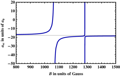
Figure 1: (Color online) Scattering length $a_{\rm sc}$ as a function of the external magnetic field value $B$ for ⁶Li-⁸⁷Rb scattering at $E=50\,$Hz. A broad and a narrow MFR are visible at $B_{0}=1066,917\,$G and $B_{0}=1282.576\,$G. The horizontal line marks the background scattering length $a_{\rm bg}=-17.8\,a_{0}$ of the left resonance.

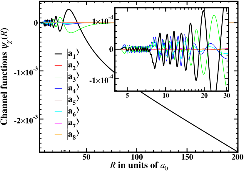
(a) (b)

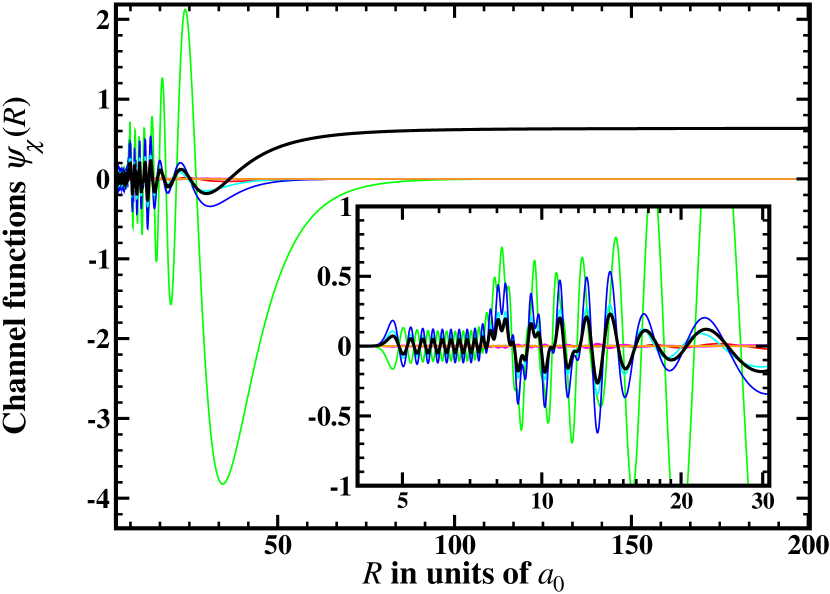
Figure 2: (Color online) The channel functions $\psi_{\chi}(R)$ for the ⁶Li-⁸⁷Rb collision in an off-resonant field $B=1000\,$G (a) and a field $B=1066.9\,$G close to the resonance (b). The atomic labels (see Tab. 1) are indicated in (a). The insets focus on a region of small internuclear distance.

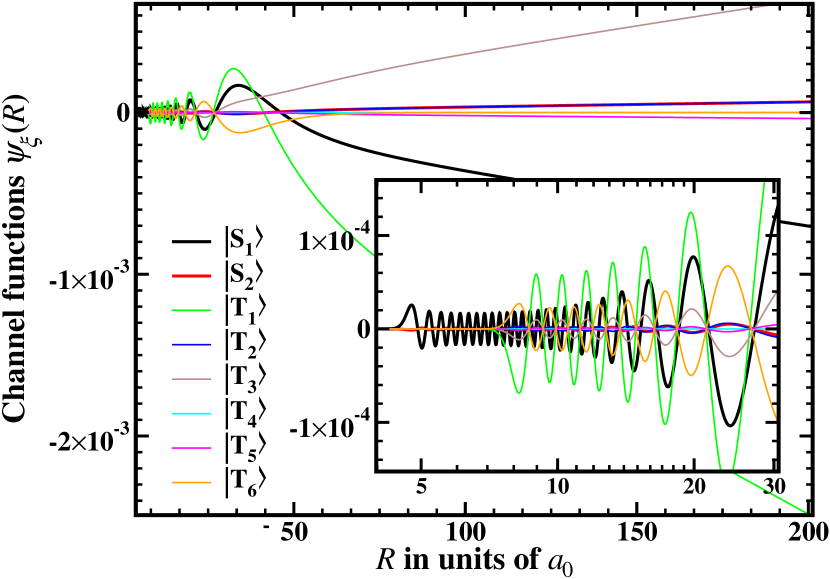
(a) (b)

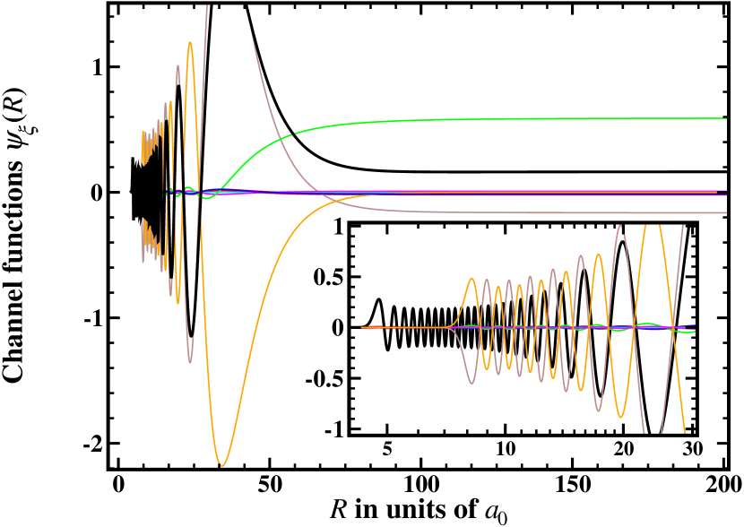
Figure 3: (Color online) The channel functions $\psi_{\xi}(R)$. The same as Fig. 2 but in MB. The molecular labels are indicated in (a).

While the narrow resonance is also examined, this paper focuses on MC solutions around the broad resonance. This resonance has been also observed experimentally Deh et al. (2008) and is well reproduced by the MC calculations. Moreover, processes like, e. g., PA are more efficient for a broad resonance because three-body losses can be minimized in this case.

Figures 2 and 3 present the channel functions of the MC calculations in AB and MB, respectively, for a collision of ⁶Li-⁸⁷Rb at two different magnetic field strengths $B$. Figures. 2(a) and 3(a) show the case of a far off-resonant field of $B$=1000 G which results in a small scattering length of only $a_{\rm sc}=-14.9\,a_{0}$. Figures 2(b) and 3(b) are taken close to the resonance at $B$=1066.9 G with a scattering length of $a_{\rm sc}=-65\ 450\,a_{0}$. This large value is arbitrarily chosen for the present study. It is already a good representation of the resonant case $a_{\rm sc}=-\infty$.

The change of the long-range behavior between two scattering situations with small and large $a_{\rm sc}$ can be more clearly analyzed in the AB where all but one channel are closed, i. e., decay for large internuclear separations (see Fig. 2). As is evident from Figs. 2(a) and (b) the open-channel wave function $\psi_{a_{1}}$ changes the slope resulting in a plateau when changing $a_{\rm sc}$ from small to large. Furthermore, the resonant open-channel function has a much larger amplitude within the considered range of interatomic distances than the off-resonant one. This large difference in amplitudes (about four orders of magnitude) sustains in the region of small internuclear distances (see insets of Figs. 2(a) and 2(b)).

At small internuclear distances above $R\approx 7\,a_{0}$ the channel functions in the AB show quite irregular behaviors (see insets of Fig. 2), which is a result of the large coupling proportional to the exchange energy $V_{\rm ex}(R)$. In the MB the coupling between the channels is induced by the hyperfine interaction that is much smaller. Hence, the channel functions show a clear behavior of pure singlet and triplet wave functions for small internuclear distances (see insets of Fig. 3). For distances $R\leq 7\,a_{0}$ the triplet components vanish due to their higher exchange energy. Accordingly, also in the AB the channel functions are similar to pure singlet wave functions at $R\leq 7\,a_{0}$ (see insets of Fig. 2). All channel functions in the MB contribute correspondingly to the decomposition of the open channel $\psi_{a_{1}}$ into states of the MB. Therefore, at large internuclear distances they look similar to $\psi_{a_{1}}$. It is important to note that at small distances the closed channel functions have non-zero amplitudes even in the $B$-field-free case; they are slightly excited during the collision and possess a background contribution to the scattering process. Therefore, the two-body collision is a multi-channel process even in field-free space.

Due to the resonant coupling at $B$=1066.9 G, the admixture of the closed channels increases about four orders of magnitude. This is well described by the TC approximation Feshbach (1958); Köhler et al. (2006) where the admixture of the closed channel and the long-range behavior of the open channel show a similar dependence on the scattering length (see Sec. II.4). In contrast to the TC approximation where one assumes that a bound state composed of a superposition of all closed channels is simply scaled at the resonance, the relative amplitudes change in reality between the resonant and off-resonant cases. On the other hand, the functional form of all closed channels indeed stays constant (compare, e. g., channel $|a_{4}\rangle$ in Figs. 2(a) and 2(b)). Altogether, this gives hope to be able to reproduce the change of the amplitude of both the open channel and the closed channels at small internuclear distances around an MFR with just one SC wave function.

II.4 Two-channel approximation

The TC approximation is very successfully used to describe resonance phenomena in MC problems Feshbach (1958); Köhler et al. (2006); Pellegrini et al. (2008). It is briefly introduced in order to understand to what extent SC approaches can mimic MC systems. A more rigorous introduction may be found in Friedrich (1991); Marcelis et al. (2004); Schneider and Saenz .

Within the TC approximation one projects the MC Hilbert space onto two subspaces, the one of the closed channels (with projection operator $\hat{\rm Q}$) and the one of the open channel (with projection operator $\hat{\rm P}$). The full wave function is thus written as $|\Psi\rangle=(\hat{\rm P}+\hat{\rm Q})|\Psi\rangle=|\Psi_{P}\rangle+|\Psi_{Q}\rangle$. An MFR occurs, if the energy $E$ of the system is close to the eigenenergy $E_{0}(B)$ of a bound state $|\Phi_{b}\rangle$ of the closed-channel subspace. In the one-pole approximation one effectively assumes that the closed-channel wave function is simply a multiple $A$ of the bound state $|\Phi_{b}\rangle$, i. e., $|\Psi_{Q}\rangle=A\,|\Phi_{b}\rangle$. This approximation yields the closed-channel admixture Schneider and Saenz

$$A=-\tilde{C}\sqrt{\frac{2}{\pi\Gamma}}\sin\delta_{\rm res}$$ (11)

where $\tilde{C}$ is a normalization constant. The long-range behavior of the open channel is given as

$$\left.\Psi_{P}(R)\right|_{R\rightarrow\infty}=\tilde{C}\sqrt{\frac{2\mu}{\pi k}}\sin(kR+\delta_{\rm bg}+\delta_{\rm res})\,.$$ (12)

If the wave function is $\sin$ normalized, then $\tilde{C}=\sqrt{\frac{\pi k}{2\mu}}$. Another popular choice is the energy normalization with $\tilde{C}=1$. However, the presence of an external trap can also induce a dependence of the normalization on the long-range behavior of the open channel parameterized by $a_{\rm sc}$, such that in general $\tilde{C}=\tilde{C}(a_{\rm sc})$.

The total phase shift $\delta=\delta_{\rm bg}+\delta_{\rm res}$ results from the background phase shift $\delta_{\rm bg}$ of the open channel without coupling to the closed channels and from a contribution $\delta_{\rm res}$ due to the resonant coupling to the bound state. Via Eq. (10) the total phase shift is connected to the scattering length $a_{\rm sc}$. The TC approximation yields for $k\rightarrow 0$ the well known relation Moerdijk et al. (1995)

$$a_{\rm sc}=a_{\rm bg}\left(1+\frac{\Delta B}{B-B_{0}}\right)$$ (13)

between scattering length and magnetic field strength, where $a_{\rm bg}=-\tan{\delta_{\rm bg}}/k$ is the background scattering length, $\Delta B$ is the width of the resonance, and $B_{0}$ its position.

We note that independently of the normalization function $\tilde{C}(a_{\rm sc})$ both the admixture of the closed channel $A$ and the long range open-channel solution (12) show for small energy, not too large internuclear distances (i. e., $kR\ll\delta$), and small background phase shifts (i. e., $\delta\approx\delta_{\rm res}$) a similar dependence on the scattering length $a_{\rm sc}$.

Usually, for small energy $E$ the background phase shift $\delta_{\rm bg}=-\arctan(ka_{\rm bg})$ is necessarily also small. Since a scaling of the open-channel wave function in the long range is more or less directly continued to shorter distances, the proportionality between $A$ and $\Psi_{P}(R)$ holds approximately also for smaller $R$. Therefore, looking at molecular processes taking place at small internuclear distances, the enhancement of the closed-channel contribution is already reproduced by the open channel. This paves the way to an SC description which will now be discussed.

III Single-channel approaches

III.1 Variations of the single-channel Hamiltonian

In order to reflect the molecular behavior at small distances, we will seek to base the SC approximations on pure singlet or triplet interaction potentials. This ensures that the nodal structure of the resulting SC wave function is similar to the relevant singlet or triplet components of the MC system. The final aim is to mimic in parallel the long-range behavior of the open channel and the variation of the amplitude of singlet or triplet components in the vicinity of an MFR.

In an SC approach the interaction strength can be artificially varied by a controlled manipulation of the Hamiltonian

$$H(R)=-\frac{1}{2\mu}\frac{\partial^{2}}{\partial R^{2}}+V(R)\,.$$ (14)

Subject to modification are the inter-atomic potential $V(R)$ and the reduced mass $\mu$ of the system. The modifications can lead to a shift of the energy of the least bound state relative to the potential threshold. When lifted above the threshold, the bound state turns into a virtual state Newton (2002); Marcelis et al. (2004). A large scattering length of the solution of the SC Schrödinger equation with Hamiltonian (14) can be elegantly explained by a resonance of the scattering state with either a real bound state or a virtual state close to the threshold Newton (2002); Marcelis et al. (2004). Within an SC approach the energy of a bound or virtual state is changed in order to induce a variation of the scattering length. In this respect SC approaches show striking similarities to MFRs where the energy of a bound state in the closed-channel subspace is moved by changing its Zeeman energy by an external magnetic field.

As argued before, the SC wave functions should be either of singlet or triplet character for small internuclear distances. We reduce our considerations for Li-Rb to the singlet case and chose as initial potential the one for the $X^{1}\Sigma^{+}$ electronic ground state, i. e., $V(R)=V_{X^{1}\Sigma^{+}}(R)$. This potential is varied by a controlled manipulation of the strong-repulsive inner wall Grishkevich and Saenz (2009), the long-range van der Waals attraction $V_{\rm vdW}(R)$ Ribeiro et al. (2004a), and a novel Gaussian perturbation around the transition point $R_{\rm sh}$ between the molecular and the atomic description of the system (introduced in Sec. II.1.2). These procedures will be called $s$ variation, $C_{6}$ variation, and $G$ variation, respectively.

The potential variations are induced by replacing $V(R)$ by

$$V^{s}(R)=\begin{cases}V(R-s\cdot\frac{R-R_{e}}{R_{c}-R_{e}})&R\leq R_{e}\\ V(R)&R>R_{e}\end{cases}\,,$$ (15)

$$V^{\delta G}(R)=V(R)+\delta G\,{\rm Exp}{\left(\frac{R-R_{G}}{\sigma}\right)^{2}}\,,$$ (16)

or

$$V^{\delta C_{6}}(R)=V(R)+\frac{\delta C_{6}}{R^{6}}\cdot f(R)$$ (17)

where $R_{e}=6.5\,a_{0}$ is the equilibrium distance and $R_{c}=4.6\,a_{0}$ is the crossing point of the $V_{X^{1}\Sigma^{+}}(R)$ with the threshold. The width in the $G$ variation is chosen as $\sigma=2\,a_{0}$ and its position as $V_{G}=R_{\rm sh}+\sigma$. The smooth variation of the long-range region of the potential in the $C_{6}$ variation is achieved by the gradual stepping function

$$f(R)=\left(1+e^{\frac{\gamma(R_{0}-R)}{\Delta}}\right)^{-1}$$ (18)

where $\gamma=\ln(999)\approx 6.9$ ensures that $f(R)$ rises from 0.001 to 0.999 in the region $R_{0}-\Delta\leq R\leq R_{0}+\Delta$. For the present study the parameters of the tuning function are chosen as $\Delta=6$ and $R_{0}=16a_{0}$. The three potential variations are depicted in Fig. 4.

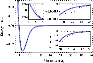
Figure 4: (Color online) Original $X^{1}\Sigma^{+}$ potential $V(R)$ (blue solid) with applied s variation (black solid), $C_{6}$ variation (dashes) and $G$ variation (dots). The variation parameters are $s=0.03\,a_{0}$, $\delta C_{6}=C_{6}/2$ and $\delta G=V(R_{\rm sh})$ (see Tab. 2 for the adopted parameters). The insets show some relevant ranges of $R$ on an enlarged scale.

An alternative way to tune $a_{\rm sc}$ is offered by the $\mu$ variation within which one changes the reduced mass of the system by $\mu\rightarrow\mu-\delta\mu$ Grishkevich and Saenz (2007). This alters the kinetic energy operator and can modify the energy of the least bound state like potential variations. In contrast to the presented potential variations which act on either the short-range, mid-range or long-range part of the potential, the mass variation influences the Schrödinger equation at any distance. It is very similar to a scaling of the potential by $V(R)\rightarrow\gamma V(R)$ Esry et al. (1999). The only difference is an additional change of the energy-momentum relation $E(k)=k^{2}/(2\mu)$ which can, e. g., slightly influence the normalization of the wave function.

One can think of several other approaches to vary the SC Hamiltonian. For example, one can vary the strength of the exchange energy $J_{0}$, its decay parameter $\alpha$ or the van der Waals parameters $C_{8},C_{10}$ Ribeiro et al. (2004a, b). The current approaches are chosen to comprise variations that act on the short rage of interatomic distance ($s$ variation), on an intermediate range ($G$ variation), on the long range ($C_{6}$ variation), and on the full range ($\mu$ variation).

No matter which SC approach is finally chosen, a mapping between the MC system and an appropriate SC Hamiltonian is straightforward. Knowing the parameters $\Delta B$ and $B_{0}$ in Eq. (13) for an MFR either from experimental data or a coupled MC calculation one can connect each value of the magnetic field $B$ to a scattering length $a_{\rm sc}$ and a corresponding value of the SC variation parameter that induces the same value of the scattering length. Clearly, this additional information is required, i. e., the SC model has no predictive power by itself.

Typical values of the four variation parameters as they will be used in the following are given in Tab. 2. The wave functions resulting from the different variation methods are denoted $\phi^{\upsilon}(R)$ where $\upsilon\in\{s,G,C_{6},\mu\}$ stands for the applied $\upsilon$ variation.

Table 2: Values of the parameters for $s,C_{6},G,\mu$ variations at small and large scattering lengths resulting from a magnetic field far away, close and right at an MFR. An infinitesimally small change of the field right at the resonance ($B=1066.92\,a_{0}$) switches the interaction regime from the infinitely attractive ($a_{\rm sc}=-\infty$) to infinitely repulsive ($a_{\rm sc}=+\infty$).

$B/$Gauss	$a_{\rm sc}/a_{0}$	$s/a_{0}$	$\delta C_{6}/C_{6}$	$\delta G/|V(R_{\rm sh})|$	$\delta\mu/\mu$
1000.00	-14.93	-0.00947	-0.0281	-0.1310	-0.00235
1066.90	-65450	-0.04142	-0.1282	-0.6296	-0.01046
1066.92	$-\infty$	-0.04145	-0.1283	-0.6302	-0.01047
	$+\infty$	0.13065	0.3357	-4.3856	0.02984

III.2 Multi-channel vs single-channel

In the following, the wave functions of the SC and MC approaches are compared. As discussed in Sec. II.1.2, the appropriate choice of the MC basis depends on the interatomic distance. While for large interatomic distances ($R>R_{\rm sh}$) the description in the AB is adequate, their basis states are strongly coupled for shorter distances. Here, the MB describes the physical properties far better. Due to the weak hyperfine coupling the states in the MB keep to a good degree of accuracy the structure of an uncoupled singlet or triplet state, respectively. Close to an MFR solely amplitudes for some of the states are heavily increased. Figure 5 shows for example a comparison of the singlet state $|S_{1}\rangle$ close to an MFR with the same state far away from the resonance and with the other singlet state $|S_{2}\rangle$ again close to the resonance. Clearly, for $R<R_{\rm sh}$ they differ only by a constant prefactor. This is important, as it allows to describe the short-range behavior of the MC wave function by either a pure singlet or triplet channel function depending on the physical process which is to be described. For example, only singlet components contribute to the DPA process for the transition into the absolute vibrational ground state (as it will be discussed in Sec. IV), hence, the triplet components may be omitted.

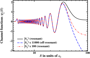
Figure 5: (Color online) The channel functions of the singlet state $|S_{1}\rangle$ close to the resonance ($a_{\rm sc}=-65\ 450\,a_{0}$) and away from the resonance ($a_{\rm sc}=-14.9\,a_{0}$) are depicted together with the channel function of the close to resonant $|S_{2}\rangle$ state. All three functions differ for $R<30\,a_{0}$ only by a constant prefactor.

In the following, the aim of the SC approach is to mimic the behavior of the MC singlet components for $R<R_{\rm sh}$ by a controlled variation of the SC Hamilton operator (14) with singlet potential $V_{X^{1}\Sigma^{+}}(R)$. With the help of the $s,C_{6},G$ and $\mu$ variations presented in Sec. III.1 the SC wave function is adjusted to match the asymptotic behavior (i. e., the scattering length $a_{\rm sc}$) of the open channel for a given external magnetic field $B$. The cases of an off-resonant magnetic field ($B=1000.0\,$G) and one close to a resonance $(B=1066.9\,$G) are considered. The corresponding scattering lengths are $a_{\rm sc}=-14.9\,a_{0}$ and $a_{\rm sc}=-65\ 450\,a_{0}$ (see Sec. II.3 and Figs. 3, 2).

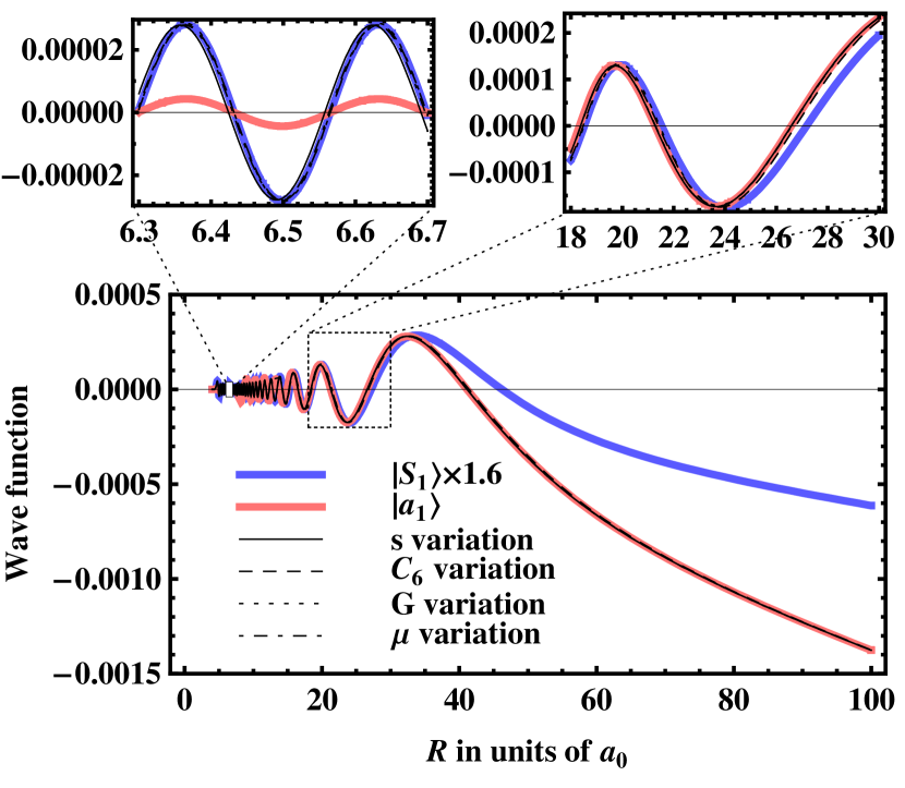
(a) (b)

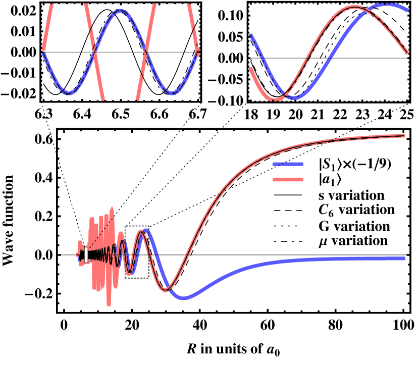
Figure 6: (Color online) Comparison of the SC wave functions $\phi^{\upsilon}(R)$ with the MC functions of the singlet state $|S_{1}\rangle$ (scaled) and the open channel $|a_{1}\rangle$. The SC potentials are varied to match the asymptotic behavior of the MC channel functions of the open channel. (a) Off-resonant case with $a_{\rm sc}=-14.9\,a_{0}$ ($B=1000\,$G). (b) Resonant case with $a_{\rm sc}=-65\ 450\,a_{0}$ ($B=1066.9\,$G). The according values of the $s,\delta C_{6},\delta G$, and $\delta\mu$ parameter are given in Tab. 2. The smaller plots focus respectively on a region of small internuclear distance (left) and a region $R\approx R_{\rm sh}$ (right).

Figure 6 shows a comparison of the SC wave functions $\phi^{\upsilon}(R)$ with the channel functions of the dominant singlet channel $|S_{1}\rangle$ and the open channel $|a_{1}\rangle$ for the full range of short and long interatomic distances. Figure 6 allows to examine how the different variational methods are able to reflect both the behavior of the singlet components for distances $R<R_{\rm sh}$ and the one of the open channel for $R>R_{\rm sh}$.

Generally, any SC approach has to induce a shift of the phase $\delta$ in order to tune the scattering length $a_{\rm sc}=-\tan(\delta)/k$. The difference $\delta-\delta_{\rm ini}$ from the phase of the unperturbed system $\delta_{\rm ini}$ is accumulated where the variation of the SC Hamiltonian takes place. Since the scattering length of the original singlet potential $V_{X^{1}\Sigma^{+}}(R)$ is with $a_{\rm sc}^{\rm ini}=2.3\,a_{0}$ relatively close to $a_{\rm sc}=-14.9\,a_{0}$, hardly any phase shift has to be acquired ($\delta-\delta_{\rm ini}=8.6\cdot 10^{-5}\pi$) to match the open channel for the off-resonant magnetic field $B=1000\,$G. Accordingly, the nodal structure of the MC singlet component is very well matched in Fig. 6(a). The situation changes close to the resonance where the large scattering length $a_{\rm sc}=-65\ 450\,a_{0}$ requires a phase shift of $\delta-\delta_{\rm ini}=0.22\pi$ (Fig. 6(b)). This is about half way to the resonant phase shift $\pi/2$.

For the $s$ variation the total phase shift to match the open channel is acquired for distances $R<6.5\,a_{0}$. Accordingly, the nodal structure between the $|S_{1}\rangle$ channel function and the SC $\phi^{s}(R)$ wave function is shifted for $R>6.5\,a_{0}$ (see upper left plot in Fig. 6(b)). Contrarily, both the $C_{6}$ variation and the $G$ variation induce a phase shift for distances $R$ larger than $R_{G}-\sigma=20\,a_{0}$ and $R_{0}=16\,a_{0}$. Thus, for smaller internuclear distances, the SC wave functions $\phi^{G}(R)$ and $\phi^{C_{6}}(R)$ coincide with the $|S_{1}\rangle$ channel function. Finally, since the $\mu$ variation acts on any internuclear distance, the phase difference is gradually accumulated for $\phi^{\mu}(R)$.

Depending on the range of variation for the SC approaches, also the matching to the open channel of AB differs. The $s$ variation matches the open channel already closely before $R_{\rm sh}$. Surprisingly, also the $\mu$ variation shows a reasonable match already before $R_{\rm sh}$, although it acts also for larger distances by changing at least the dispersion relation $E(k)$. This effect may, however, not be visible, since $kR\ll 1$ in the plotted region. The $C_{6}$ variation changes the long-range behavior of the interaction potential. Correspondingly, the wave function shows a clear difference to the open channel even up to $R=100\,a_{0}$. The Gaussian perturbation of the G variation acts only around $R_{\rm sh}$. This results in the favorable situation that both the $|S_{1}\rangle$ channel for $R<20\,a_{0}$ and the open channel for $R>24\,a_{0}$ are matched by the SC wave function.

Since the nodal structure among different singlet and different triplet channels coincides for $R<R_{\rm sh}$ the presented results are generalizable to any singlet or triplet state. Thus, SC approaches are generally able to reproduce the asymptotic behavior of the open channel of the MC wave function in the presence of an MFR while also reflecting certain aspects of singlet or triplet components for small internuclear distances. Depending on the region of the variation of the SC Hamiltonian, the nodal structure of any channel function in the MB can be reproduced for $R<R_{\rm sh}$. The most flexible SC approach is the $G$ variation which is able to smoothly switch between the accurate description of a MB channel and the open channel. Furthermore, it offers the advantage, that one can define the transition point (here $R=R_{\rm sh}$) at will, such that also for slightly larger distances MB channel functions can be emulated.

An aspect of the MB channels which cannot be reflected by the present approaches is their absolute amplitude. Since the amplitudes at small internuclear distances of the different channels change drastically in the presence of an MFR, they have a large impact on molecular processes such as the association of molecules utilizing MFRs. In the next section the exemplary case of a direct dumping of the scattering state to the vibrational ground state of the $X^{1}\Sigma^{+}$ is considered. The transition rate depends strongly on the behavior of the amplitude of the dominant singlet state $|S_{1}\rangle$ which was considered in this section. It will be shown that although the absolute amplitude of this state is not reproduced by any SC approach, the relative enhancement of the transition rate at magnetic fields close to a resonance can be well reflected.

IV Photoassociation of ⁶Li-⁸⁷Rb to the absolute vibrational ground state

Ultracold polar molecules are of great interest for many applications in quantum information processing Micheli et al. (2006); Rabl et al. (2006), the exploration of lattices of dipolar molecules Pupillo et al. (2008), precision measurement of fundamental constants Zelevinsky et al. (2008), and ultracold chemical reactions Chin et al. (2005); Tscherbul and Krems (2006). Since standard cooling technics developed for atoms are not suitable for molecules due to their complex level structure, ultracold molecules may alternatively be associated directly from ultracold atoms. As was already mentioned in the introduction the starting point to create ultracold molecules in their vibrational ground state are often Feshbach molecules formed by a sweep of the magnetic field around an MFR in a high-lying vibrational level Köhler et al. (2006). These loosely bound molecules are usually transferred by complex PA schemes via intermediate excited states to the desired vibrational ground state Ni et al. (2008); Sage et al. (2008). Especially STIRAP Bergmann et al. (1998); Winkler et al. (2008); Ospelkaus et al. (2008); Danzl et al. (2008) showed to be successful in efficiently creating ultracold ground state molecules. However, Feshbach molecules possess a relatively short life time such that a Feshbach optimized transition directly at the resonance can be favorable Kuznetsova et al. (2009).

For all schemes that make advantage of the resonant coupling to a molecular bound state at an MFR van Abeelen et al. (1998); Courteille et al. (1998); Regal et al. (2003); Grishkevich and Saenz (2007); Junker et al. (2008); Pellegrini et al. (2008); Deiglmayr et al. (2009), the increase of the amplitude for the relevant channels as the scattering length grows is of great importance to enhance the molecule creation. Although in the last section it was shown that the absolute amplitude of the MB channels is not reproduced by the SC approaches, the TC approximation gives hope that the relative enhancement can still be recovered. In Sec. II.4 it was discussed that both the admixture of the closed-channel bound state and the open-channel function scale similarly with the scattering length. One can therefore expect to be able to combine this collective relative enhancement into one channel.

In the following, the Feshbach optimized DPA (FOPA) Kuznetsova et al. (2009) to the absolute vibrational ground state of ⁶Li-⁸⁷Rb in the electronic $X^{1}\Sigma^{+}$ state is considered to examine the applicability of SC approaches to study processes of molecule creation. We consider this case since it has an interest on its own for the creation of bound ultracold molecules. Furthermore, the transition rate to the absolute vibrational ground state depends on the scattering wave function at very small internuclear distances (see Fig. 7). We also examined the transition to the vibrational ground state of the electronic triplet state $a^{3}\Sigma^{+}$ which is situated at slightly larger interatomic distances. Since we found no essential differences to the singlet case, we focus on presenting only its results in this work.

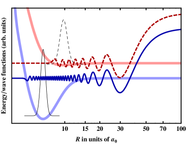
Figure 7: (Color online) Sketch of the resonant SC wave functions obtained via $G$ variation and respective BO potentials relevant for the DPA transition to either the singlet ground state (thin, solid) or the triplet ground state (thin, dashed) of the respective $X^{1}\Sigma^{+}$ (thick, blue) and $a^{3}\Sigma^{+}$ (thick, red) potentials. For better visibility, the potentials and wave functions are shifted along the y-axis. In reality, singlet and triplet potentials have the same threshold energy.

IV.1 Calculation of transition rates

Given the solution of the MC problem $\Psi(R)=\sum_{\xi}\frac{\psi_{\xi}(R)}{R}|\xi\rangle$ in the MB for a given magnetic field $B$ the free-bound FOPA transition rate $\Gamma_{\downarrow}(B)$ to the final molecular state $\Psi_{\rm f}(R)=\frac{\Psi_{\nu}(R)}{R}Y_{J}^{M}(\Theta,\Phi)|\xi_{\rm f}\rangle$ with vibrational quantum number $\nu$ and rotational quantum number $J$ within the dipole approximation is proportional to the squared dipole transition moment Sando and Dalgarno (1971)

$$I_{\rm MC}(B)=\left|\int\limits_{0}^{\infty}\Psi_{\nu}(R)D(R)\psi_{\xi_{\rm f}}(R)dR\right|^{2}\,.$$ (19)

Here, $D(R)$ is the electronic dipole moment. Within the dipole approximation only transitions from the s-wave scattering function to a final state with $J=1$ are allowed. Due to the orthogonality of the MB, only one molecular channel has to be taken into account in Eq. (19).

The TC approximation predicts a rate Schneider and Saenz

$$I_{\rm TC}(B)=|\tilde{C}\cdot\mathcal{C}|^{2}\cdot\left|\sin\left(\delta_{\rm res}(B)-\delta_{0}\right)\right|^{2}$$ (20)

where the constants $\mathcal{C}$ and $\delta_{0}$, explicitely given in Schneider and Saenz , do not depend on the magnetic field within the TC approximation. The phase shift $\delta_{0}$ is usually small Schneider and Saenz and thus the minimum lies close to a vanishing resonant phase shift $\delta_{\rm res}=0$, i. e., close to the background scattering length $a_{\rm bg}$. We determine $a_{\rm bg}$ by a fit of $a_{\rm sc}(B)$ to Eq. (13) which yields $a_{\rm bg}=-17.8a_{0}$. From $\delta=\delta_{\rm res}+\delta_{\rm bg}$ and Eq. (13) one can then directly determine $\delta_{\rm res}(B)$. The behavior of Eq. (20) accurately reflects the one of a MC system for well separated resonances Schneider and Saenz . We use it here to determine the maximal MC transition rate.

The transition rate $\Gamma_{\downarrow}^{\upsilon}$ to the final state within an SC approach is simply proportional to

$$I_{\rm SC}^{\upsilon}(a_{\rm sc})=\left|\int_{0}^{\infty}\Psi_{\nu}(R)D(R)\phi^{\upsilon}(R)\right|^{2}$$ (21)

where $\upsilon$, as before, denotes the variational method which for the present analysis induces the scattering length $a_{\rm sc}$ equal to the one of the MC system for a given $B$-field value.

$D(R)$ is again the electronic dipole transition moment. For the purpose of the present study we reduce our considerations to the linear approximation $D(R)=D_{0}+D_{1}\cdot R$. The SC scattering wave function is orthogonal to the different vibrational bound states. In the MC case only the weak hyperfine coupling in the MB causes a very slight non-orthogonality. The influence of $D_{0}$ can be therefore safely ignored. Calculations with higher-order expansions showed that the exact functional behavior of $D(R)$ (obtainable from Aymar and Dulieu (2005)) does hardly influence the relative enhancement of the transition rate. Thus, the use of $D(R)=D_{1}\cdot R$ does not restrict generality. It is important to note that Eqs. (19)-(21) are only valid within the dipole approximation. It is supposed to be applicable, if the wavelength of the associating photon is much larger than the spatial extension of the atomic or molecular system. The shortest PA laser wavelength corresponds to the transition to the lowest vibrational state. Although the spatial extention of the initial state is infinite, the integrals for dipole transition moments is finite, as it contains a finite wave function of the bound vibrational state as a factor. Therefore the dipole approximation is valid.

IV.2 Comparison of transition rates

A change of $a_{\rm sc}$ leads to an increase or decrease of $\Gamma_{\downarrow}^{v}$. In order to quantify the magnitude of this change, an enhancement or suppression factor may be introduced Grishkevich and Saenz (2007)

$$g^{v}(a_{\rm sc})=\frac{\Gamma_{\downarrow}^{v}(a_{\rm sc})}{\Gamma_{\downarrow}^{v}(a_{\rm sc}^{\rm ref})}=\frac{I^{v}(a_{\rm sc})}{I^{v}(a_{\rm sc}^{\rm ref})}\quad.$$ (22)

It describes the relative enhancement [$g^{v}>1$] or suppression [$g^{v}<1$] of the DPA rate at a given $a_{\rm sc}$ vs. a reference scattering length $a_{\rm sc}^{\rm ref}$, for a specific final state $v$. Although it may appear to be most natural to choose $a_{\rm sc}^{\rm ref}=0$, a large non-zero value offers some advantages. In this case, $I^{v}(a_{\rm sc}^{\rm ref})$ is not too small and large numerical errors are avoided.

Figure 8 shows a comparison of the SC transition rate for the different variational approaches with the correct MC result. In the calculation of the MC transition rates, we assume a measurement in which the nuclear spins are not resolved. This corresponds in practice to the case in which the transition rates from the $|S_{1}\rangle$ and $|S_{2}\rangle$ channel are summed. All rates are normalized to their respective maximum value ($a_{\rm sc}^{\rm ref}=\infty$). Note, however, that the different absolute dipole transition moments disagree by some orders of magnitude.

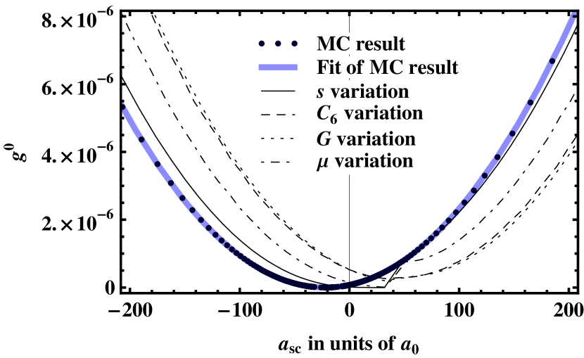
(a) (b)

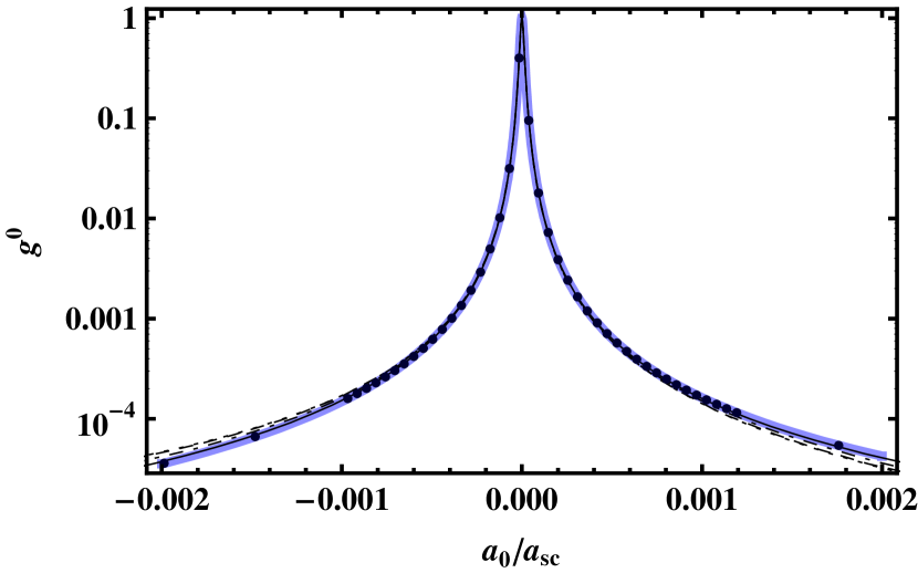
Figure 8: (Color online) Comparison of MC and SC results for the transition rate to the absolute vibrational ground state relative to the respective maximal transition rate as a function of the scattering length (a) and the inverse scattering length (b). The MC results are fitted according to the TC approximation (Eq. (20)).

A fit of the MC result by the TC estimate with only two free parameters $\mathcal{C}$ and $\delta_{0}$ reveals that the simple dependence of the transition rate given by Eq. (20) describes the transition process of the MC system correctly.

All SC approaches agree with the MC result for large scattering lengths in the proximity of the resonance (see Fig. 8(b)). For small scattering lengths where the transition rate is already suppressed by more than four orders of magnitude deviations from the MC result appear. The differences mainly originate from a shift of the minimal transition rates of the SC approaches compared to the MC result. In the MC case the minimum lies at $a_{\rm sc}=-21.1a_{0}$ close to the background scattering length $a_{\rm bg}=-17.8a_{0}$ in accordance with the TC approximation. The minima of the SC approaches tend to be situated on the positive side around $a_{\rm sc}\approx 50a_{0}$. This is, however, not a general trend, since we observed for other transitions also minimal SC transition rates at negative scattering lengths. The location of the minimum depends on a system under investigation and on the applied SC variation.

Figure 8(a) features two kinks of the transition rate at $a_{\rm sc}=40\,a_{0}$ for the $s$ and $\mu$ variations. This can be explained by the shift of the nodes of the SC wave functions which takes place at the equilibrium distance of the bound molecule and therefore influences the PA rate. Since the variation parameters are tuned around their resonance value, with increasing distance from the resonance both left and right of it, eventually the same scattering length is induced (see Fig. 9). However, the nodal structure of $\phi^{s}(R)$ and $\phi^{\mu}(R)$ for short ranges can differ, leading to different transition rates. This does not occur for the $C_{6}$ and $G$ variations that act far beyond the equilibrium distance. Note, however, the scale at which the kink is visible. Its effect on the rate is minute.

Analogous examinations were also done for the other MFR of ⁶Li-⁸⁷Rb at $B=1282.58\,$G. Although this resonance is two orders of magnitude narrower than the one considered before and the amplitudes of the channels are different, no significant differences for the relative rates were observed. The generality of our considerations is also supported by calculations of the dumping rate to the vibrational ground state of the triplet configuration $a^{3}\Sigma^{+}$. In all cases the SC approaches showed a comparable ability to reflect results of the MC system.

It is also interesting to note that results of the $g^{0}$ analysis show that neither the details of the interatomic nor magnetic-field interactions are relevant for the calculation of the relative rate. A simple SC model turns out to be adequate to calculate the relative enhancement of the PA process. Furthermore, in view of the important question of how to optimize the efficiency of DPA, Fig. 8 reveals once more that the use of a large absolute value of the scattering length is favorable.

IV.3 Number of bound states

As already mentioned, SC resonances are evoked by artificially shifting the least bound state or a virtual state across the threshold. By turning a bound state into a virtual state or vice versa, the total number of bound states $N_{\rm b}$ changes necessarily. This can be avoided by stopping the variation just before the bound or virtual states reach the threshold. Nevertheless it is possible to achieve any scattering length by moving between two different SC resonances. This is illustrated by the example of the $\mu$ variation in Fig. 9(a) where three resonant branches of the $a_{\rm sc}(\delta\mu)$ curve are depicted. As discussed in Grishkevich and Saenz (2007) the question arises, whether it is preferable to keep $N_{\rm b}$ constant or to change the variation parameter across a SC resonance as was done so far in this work.

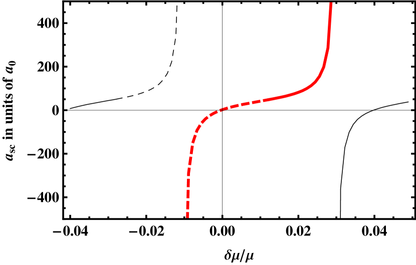
(a) (b)

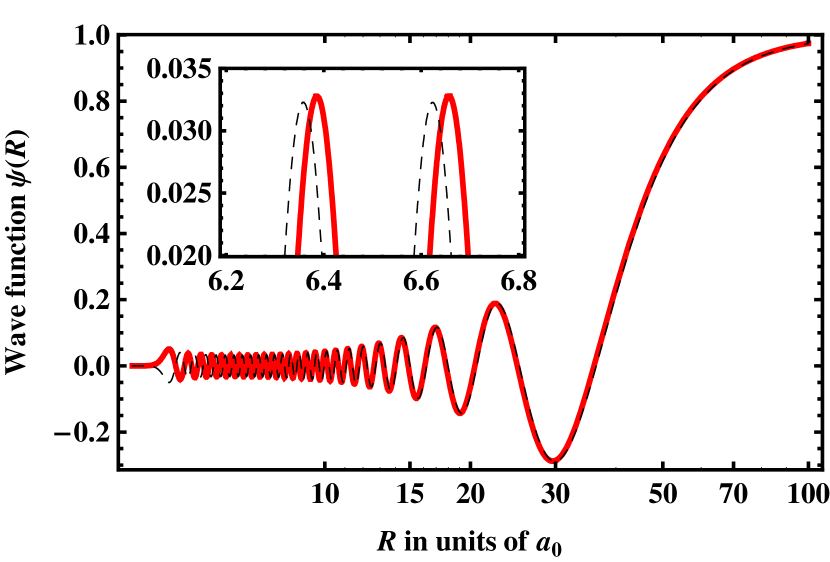
Figure 9: (Color online) (a) Scattering length $a_{\rm sc}$ as a function of the $\delta\mu$-parameter of the mass variation. By constraining the variation to the thick (red) branch, any scattering length is reached while keeping the number of bound states $N_{\rm b}$ constant. By constraining it to the dashed (black/red) branch any scattering length is reached while $N_{\rm b}$ changes. (b) Resonant SC functions ($a_{\rm sc}=\infty$) at two different $\delta\mu$-parameters $\delta\mu\approx-0.01\mu$ (dashed), $\delta\mu\approx 0.03\mu$ (thick, red). In order to make the relevant phase and amplitude difference at small internuclear distances visible one of the wave function is multiplied by $-1$ in the inset.

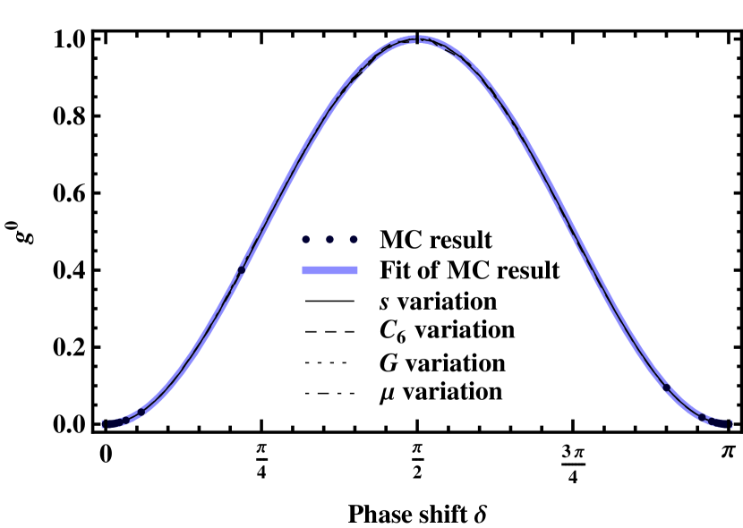
(a) (b)

Figure 10: (Color online) Comparison of MC and SC results for the transition rate $I^{0}$ to the absolute vibrational ground state relative to the respective maximal transition rate as a function of the phase shift $\delta$. The different SC variation parameters are either varied around one SC resonance (a) or between two resonances staying on the same $a_{\rm sc}(\delta\mu)$ branch (b). The MC results are fitted, according to the TC approximation (Eq. (20)). Note the $\sin^{2}$-like form of the functions.

In Figs. 10(a) and (b) the relative transition rate is depicted as a function of the phase shift $\delta$. In comparison to a $1/a_{\rm sc}$-plot (Fig. 8(b)), this allows an enlarged view on the region of resonance where the phase $\delta$ suddenly crosses $\pi/2$. In Fig. 10(a) the SC variations are performed in the same way as in Fig. 8 around one SC resonance while changing $N_{\rm b}$. This results in a perfect agreement with the MC result (the deviations at small relative rates as shown in Fig. 8(a) are not visible on a linear scale of the relative rate). Furthermore, large values of the scattering length can be obtained by slight modifications of the SC Hamiltonian. By fixing $N_{\rm b}$, one has to stay on the same branch of the resonant curve $a_{\rm sc}(\upsilon)$. This modifies the SC Hamiltonian strongly and can lead to a sudden change of the relative rate by some 30% as is shown in Fig. 10(b).

The reason for the sudden change of the wave function is twofold. In all cases the asymptotic behavior of the wave functions are the same at different resonant points corresponding the same $a_{\rm sc}$, but different Hamiltonians lead to a slightly different continuation of the wave function towards smaller distances. If the variation takes place at ranges larger than the equilibrium distance $R_{e}$ ($C_{6},G$ and $\mu$ variation), the wave function around $R_{e}$ where it influences directly the transition rate can differ slightly in amplitude. Secondly, if the variation takes place around $R_{e}$ ($s$ and $\mu$ variation) the nodal structure of the SC wave functions differs for both resonant SC parameters, since the necessary phase shift is acquired in different ways. Both effects induce a “step” in the transition rate at $\delta=\pi/2$ as is visible in Fig. 10(b). The nodal shift can in principle change the transition rate more strongly than in the present case. Figure 9(b) compares the two wave functions of the $\mu$ variation at different resonant $\delta\mu$ parameters. One can observe around $R\approx R_{e}$ both effects just described: the change of amplitude and the change of the nodal structure for different resonant variation parameters.

To conclude, in order to calculate relative PA rates it should be in most cases preferable not to keep the number of bound states fixed and to avoid a sudden change of the SC scattering wave function while going over the resonance. The drawback is of course a sudden change of the wave function for small scattering lengths. But here the SC approaches show in any way differences to the MC result, such as a shift of the minimal transition rate along the $a_{\rm sc}$ axis (Fig. 8(a)). Noteworthy, for the energy spectrum analysis, as it was done, e. g., in Grishkevich and Saenz (2009) for two atoms in an OL, it is more convenient to stay on the same SC resonant branch. The alternative variation with non-constant $N_{\rm b}$ does not influence the resulting energy spectrum. However, the disadvantage is that the numbering of the discrete levels should be changed across a SC resonance.

V Conclusion

We presented single-channel approaches that were able to reproduce both the long-range behavior of the open channel as well as the nodal structure and relative enhancement of any singlet or triplet state of a multi-channel system in the presence of a magnetic Feshbach resonance. However, single-channel variations induce a shift of the nodal structure not present in the multi-channel solution. Furthermore, the overall amplitude of the wave function stemming from the asymptotical behavior can be slightly modulated by long and intermediate-range variations. The $G$ variation, introduced in this work, showed to reproduce the corresponding multi-channel components at short and long interatomic distances most accurately.

As was demonstrated for the exemplary case of ⁶Li-⁸⁷Rb scattering single-channel wave functions can be used to study processes of molecule formation. We examined the specific process of a direct one-photon photoassociation to the absolute vibrational ground state of ⁶Li-⁸⁷Rb and proved the applicability of the single-channel approaches to model this process. The effects of the nodal shift and the modulation of the amplitude lead to a discontinuity in the transition rate for either small scattering lengths, if varying the single-channel Hamiltonian over a resonance, or at large scattering lengths, if keeping the number of bound states constant. As was discussed, a variation around a resonance of the single-channel Hamiltonian is preferable, since the point of minimal transition at small scattering lengths deviates in any way between multi-channel and single-channel results. These deviations appear, however, at scattering lengths where the transition rate is negligible compared to the one at resonance.

The general applicability of single-channel approaches was based on the two-channel approximation which reveals that the scaling of the open-channel wave function and the admixture of closed channels depends on the scattering length in a similar way. Additionally, by the help of this approximation one is able to reproduce exactly the multi-channel transition rate by adjusting two free parameters, that combine all details of the transition process.

We can conclude that single-channel approaches are a suitable starting ground to study molecular processes in regimes were full multi-channel calculations are too laborious. This is, e. g., the case, if the scattering takes place in an external trapping potential like an optical lattice, that in general couples relative and center-of-mass motions and spoils the spherical symmetry. In most cases the trapping potential does not directly influence the scattering wave function at short interatomic distances, but it induces an additional modulation of the amplitude as a function of the scattering length. The examination of effects due to these modulations are perfect candidates for the use of single-channel approaches.

Since the nodal structure of either the singlet or the triplet components of the multi-channel wave function is reproduced by single-channel approximations, also more complicated photoassociation schemes, exciting a range of higher vibrational states, can be examined in the presence of a trapping potential. Furthermore, single-channel approaches allow to treat three and many-body collisions with reasonable numerical efforts in the presence of a magnetic Feshbach resonance.

Of course, the presented single-channel approaches have also clear restrictions. For example, one has to assume that the scattering energy and the background scattering length are sufficiently small. This condition can be spoiled for certain atomic systems and in deep external trapping potentials with significantly large ground state energy. Another problem can be caused by the energy dependence of the scattering length especially for narrow Feshbach resonances. This energy dependence is not reflected by the current approaches. Furthermore, the multi-channel wave function might behave differently compared to the single-channel one, if an energy variation is induced by, e. g., ramping up an external trap. There exist single-channel approaches, which account for the energy dependence of the scattering length by a well-barrier pseudo-potential De Palo et al. (2004). However, like any pseudo potential it is unable to reflect the nodal structure of the scattering wave function at small internuclear distances.

Recently Deiglmayr et al. observed for ⁷Li-¹³³Cs (at $B=0$) the exceptional case of a strong deviation of molecular channel functions from pure singlet or triplet behavior at small internuclear distances Deiglmayr et al. (2009). Since spin-orbit coupling was neglected, they attributed this unusual effect to strong hyperfine coupling but gave no reason, why this happens specifically for the considered system. It is certainly interesting to further investigate this effect which would limit the applicability of single-channel wave functions to predict, e. g., the relative transition rates to different vibrational levels.

Apart from this unusual behavior it should be possible from the theoretical considerations presented in this work to determine, whether and which single-channel approach is applicable for a specific system and molecular process.

References

- Weiner et al. (1999) J. Weiner, V. S. Bagnato, S. Zilio, and P. S. Julienne, Rev. Mod. Phys. 71, 1 (1999).
- Jochim et al. (2003) S. Jochim, M. Bartenstein, A. Altmeyer, G. Hendl, S. Riedl, C. Chin, J. Hecker Denschlag, R. Grimm, C. Zhu, A. Dalgarno, et al., Science 302, 2101 (2003).
- Regal et al. (2003) C. A. Regal, C. Ticknor, J. L. Bohn, and D. S. Jin, Nature 424, 47 (2003).
- Zwierlein et al. (2003) M. W. Zwierlein, C. A. Stan, C. H. Schunck, S. M. F. Raupach, S. Gupta, Z. Hadzibabic, and W. Ketterle, Phys. Rev. Lett. 91, 250401 (2003).
- Jordens et al. (2008) R. Jordens, N. Strohmaier, K. Gunter, H. Moritz, and T. Esslinger, Nature 455, 204 (2008).
- Lett et al. (1993) P. D. Lett, K. Helmerson, W. D. Phillips, L. P. Ratliff, S. L. Rolston, and M. E. Wagshul, Phys. Rev. Lett. 71, 2200 (1993).
- Fioretti et al. (1998) A. Fioretti, D. Comparat, A. Crubellier, O. Dulieu, F. Masnou-Seeuws, and P.Pillet, Phys. Rev. Lett. 80, 4402 (1998).
- Jaksch et al. (2002) D. Jaksch, V. Venturi, J. I. Cirac, C. J. Williams, and P. Zoller, Phys. Rev. Lett. 89, 040402 (2002).
- Deb and You (2003) B. Deb and L. You, Phys. Rev. A 68, 033408 (2003).
- Grishkevich and Saenz (2007) S. Grishkevich and A. Saenz, Phys. Rev. A 76, 022704 (2007).
- Grishkevich and Saenz (2009) S. Grishkevich and A. Saenz, Phys. Rev. A 80, 013403 (2009).
- Jaksch et al. (1998) D. Jaksch, C. Bruder, J. I. Cirac, C. W. Gardiner, and P. Zoller, Phys. Rev. Lett. 81, 3108 (1998).
- Greiner et al. (2002) M. Greiner, O. Mandel, T. Esslinger, T. Hänsch, and I. Bloch, Nature 415, 39 (2002).
- Köhl et al. (2005) M. Köhl, H. Moritz, T. Stöferle, K. Günter, and T. Esslinger, Phys. Rev. Lett. 94, 080403 (2005).
- Esry et al. (1999) B. D. Esry, C. H. Greene, and J. P. Burke, Phys. Rev. Lett. 83, 1751 (1999).
- Simoni et al. (2009) A. Simoni, J.-M. Launay, and P. Soldán, Phys. Rev. A 79, 032701 (2009).
- Schneider et al. (2009) P.-I. Schneider, S. Grishkevich, and A. Saenz, Phys. Rev. A 80, 013404 (2009).
- Bloch et al. (2008) I. Bloch, J. Dalibard, and W. Zwerger, Rev. Mod. Phys. 80, 885 (2008).
- Inouye et al. (1998) S. Inouye, M. R. Andrews, J. Stenger, H.-J. Miesner, D. M. Stamper-Kurn, and W. Ketterle, Nature 392, 151 (1998).
- Köhler et al. (2006) T. Köhler, K. Góral, and P. S. Julienne, Rev. Mod. Phys. 78, 1311 (2006).
- Drummond et al. (2002) P. D. Drummond, K. V. Kheruntsyan, D. J. Heinzen, and R. H. Wynar, Phys. Rev. A 65, 063619 (2002).
- van Abeelen et al. (1998) F. A. van Abeelen, D. J. Heinzen, and B. J. Verhaar, Phys. Rev. A 57, R4102 (1998).
- Courteille et al. (1998) P. Courteille, R. S. Freeland, D. J. Heinzen, F. A. van Abeelen, and B. J. Verhaar, Phys. Rev. Lett. 81, 69 (1998).
- Junker et al. (2008) M. Junker, D. Dries, C. Welford, J. Hitchcock, Y. Chen, and R. Hulet, Phys. Rev. Lett. 101, 060406 (2008).
- Pellegrini et al. (2008) P. Pellegrini, M. Gacesa, and R. Côté, Phys. Rev. Lett. 101, 053201 (2008).
- Deiglmayr et al. (2009) J. Deiglmayr, P. Pellegrini, A. Grochola, M. Repp, R. Cote, O. Dulieu, R. Wester, and M. Weidemuller, New Journal of Physics 11, 055034 (2009).
- Ribeiro et al. (2004a) E. Ribeiro, A. Zanelatto, and R. Napolitano, Chem. Phys. Lett. 390, 89 (2004a).
- Feshbach (1958) H. Feshbach, Ann. Phys. (N.Y.) 5, 357 (1958).
- Kokkelmans et al. (2002) S. J. J. M. F. Kokkelmans, J. N. Milstein, M. L. Chiofalo, R. Walser, and M. J. Holland, Phys. Rev. A 65, 053617 (2002).
- Mies et al. (2000) F. H. Mies, E. Tiesinga, and P. S. Julienne, Phys. Rev. A 61, 022721 (2000).
- Góral et al. (2004) K. Góral, T. Köhler, S. A. Gardiner, E. Tiesinga, and P. S. Julienne, J. Phys. B: At. Mol. Phys. 37, 3457 (2004).
- Nygaard et al. (2008) N. Nygaard, R. Piil, and K. Mølmer, Phys. Rev. A 78, 023617 (2008).
- (33) P.-I. Schneider and A. Saenz, arXiv:0909.4406 (to be published).
- Burke et al. (2007) P. G. Burke, C. J. Noble, and V. M. Burke, Adv. Atom. Mol. Opt. Phys. 54, 237 (2007).
- Micheli et al. (2006) A. Micheli, G. K. Brennen, and P. Zoller, Nature 2, 341 (2006).
- Rabl et al. (2006) P. Rabl, D. DeMille, J. M. Doyle, M. D. Lukin, R. J. Schoelkopf, and P. Zoller, Phys. Rev. Lett. 97, 033003 (2006).
- Pupillo et al. (2008) G. Pupillo, A. Griessner, A. Micheli, M. Ortner, D.-W. Wang, and P. Zoller, Phys. Rev. Lett. 100, 050402 (2008).
- Moerdijk and Verhaar (1995) A. J. Moerdijk and B. J. Verhaar, Phys. Rev. A 51, R4333 (1995).
- Arimondo et al. (1977) E. Arimondo, M. Inguscio, and P. Violino, Rev. Mod. Phys. 49, 31 (1977).
- Marzok et al. (2009) C. Marzok, B. Deh, C. Zimmermann, P. W. Courteille, E. Tiemann, Y. V. Vanne, and A. Saenz, Phys. Rev. A 79, 012717 (2009).
- Li et al. (2008) Z. Li, S. Singh, T. V. Tscherbul, and K. W. Madison, Phys. Rev. A 78, 022710 (2008).
- Bransden and Joachain (2003) B. H. Bransden and C. J. Joachain, eds., Physics of atoms and molecules (Prentice Hall, England, 2003).
- Smirnov and Chibisov (1965) B. M. Smirnov and M. I. Chibisov, Sov. Phys. JETP 21, 624 (1965).
- Bhattacharya et al. (2004) M. Bhattacharya, L. O. Baksmaty, S. B. Weiss, and N. P. Bigelow, Eur. Phys. J. D 31, 301 (2004).
- Bambini and Geltman (2002) A. Bambini and S. Geltman, Phys. Rev. A 65, 062704 (2002).
- Deh et al. (2008) B. Deh, C. Marzok, C. Zimmermann, and P. W. Courteille, Phys. Rev. A 77, 010701 (2008).
- Friedrich (1991) H. Friedrich, Theoretical Atomic Physics (Springer-Verlag, Berlin, 1991).
- Marcelis et al. (2004) B. Marcelis, E. G. M. van Kempen, B. J. Verhaar, and S. J. J. M. F. Kokkelmans, Phys. Rev. A 70, 012701 (2004).
- Moerdijk et al. (1995) A. J. Moerdijk, B. J. Verhaar, and A. Axelsson, Phys. Rev. A 51, 4852 (1995).
- Newton (2002) R. Newton, Scattering theory of waves and particles (Dover Pubns, 2002).
- Ribeiro et al. (2004b) E. Ribeiro, A. Zanelatto, and R. Napolitano, Chem. Phys. Lett. 399, 135 (2004b).
- Zelevinsky et al. (2008) T. Zelevinsky, S. Kotochigova, and J. Ye, Phys. Rev. Lett. 100, 043201 (2008).
- Chin et al. (2005) C. Chin, T. Kraemer, M. Mark, J. Herbig, P. Waldburger, H.-C. Nägerl, and R. Grimm, Phys. Rev. Lett. 94, 123201 (2005).
- Tscherbul and Krems (2006) T. V. Tscherbul and R. V. Krems, Phys. Rev. Lett. 97, 083201 (2006).
- Ni et al. (2008) K.-K. Ni, S. Ospelkaus, M. H. G. de Miranda, A. Pe’er, B. Neyenhuis, J. J. Zirbel, S. Kotochigova, P. S. Julienne, D. S. Jin, and J. Ye, Science 322, 231 (2008).
- Sage et al. (2008) J. M. Sage, S. Sainis, T. Bergeman, and D. DeMille, Phys. Rev. Lett. 94, 203001 (2008).
- Bergmann et al. (1998) K. Bergmann, H. Theuer, and B. W. Shore, Rev. Mod. Phys. 70, 1003 (1998).
- Winkler et al. (2008) K. Winkler, F. Lang, G. Thalhammer, P. v. d. Straten, R. Grimm, and J. H. Denschlag, Phys. Rev. Lett. 98, 043201 (2008).
- Ospelkaus et al. (2008) S. Ospelkaus, A. Pe’er, K.-K. Ni, J. J. Zirbel, B. Neyenhuis, S. Kotochigova, P. S. Julienne, J. Ye, and D. S. Jin, Nature 4, 622 (2008).
- Danzl et al. (2008) J. G. Danzl, E. Haller, M. Gustavsson, M. J. Mark, R. Hart, N. Bouloufa, O. Dulieu, H. Ritsch, and H.-C. Nägerl, Science 321, 1062 (2008).
- Kuznetsova et al. (2009) E. Kuznetsova, M. Gacesa, P. Pellegrini, S. F. Yelin, and R. Cote, New Journal of Physics 11, 055028 (2009).
- Sando and Dalgarno (1971) K. Sando and A. Dalgarno, Mol. Phys. 20, 103 (1971).
- Aymar and Dulieu (2005) M. Aymar and O. Dulieu, J. Chem. Phys. 122, 204302 (2005).
- De Palo et al. (2004) S. De Palo, M. L. Chiofalo, M. J. Holland, and S. J. J. M. F. Kokkelmans, Phys. Lett. A 327, 490 (2004).