Thermal Response of A Solar-like Atmosphere to
An Electron Beam from A Hot Jupiter: A Numerical Experiment

Abstract

We investigate the thermal response of the atmosphere of a solar-type star to an electron beam injected from a hot Jupiter by performing a 1-dimensional magnetohydrodynamic numerical experiment with non-linear wave dissipation, radiative cooling, and thermal conduction. In our experiment, the stellar atmosphere is non-rotating and is modelled as a 1-D open flux tube expanding super-radially from the stellar photosphere to the planet. An electron beam is assumed to be generated from the reconnection site of the planet’s magnetosphere. The effects of the electron beam are then implemented in our simulation as dissipation of the beam momentum and energy at the base of the corona where the Coulomb collisions become effective. When the sufficient energy is supplied by the electron beam, a warm region forms in the chromosphere. This warm region greatly enhances the radiative fluxes corresponding to the temperature of the chromosphere and transition region. The warm region can also intermittently contribute to the radiative flux associated with the coronal temperature due to the thermal instability. However, owing to the small area of the heating spot, the total luminosity of the beam-induced chromospheric radiation is several orders of magnitude smaller than the observed Ca II emissions from HD 179949.

1 Introduction

Hot Jupiters are Jupiter-mass planets located within $\sim$ 0.1 AU or less from their parent stars. Because of the close proximity to the parent stars, hot Jupiters have been expected to be able to influence their stellar companions via magnetic (Cuntz et al., 2000; Rubenstein & Schaefer, 2000) and/or tidal interactions (Lin et al., 1996; Jackson et al., 2009; Pfahl et al., 2008). The observations of Ca II H & K lines from a number of stars harboring a hot Jupiter have suggested that the chromospheric activities, characterized either by line intensity or short-time variability, sometimes correlate with the orbits of their planets (Shkolnik et al., 2003, 2005, 2008). These phenomena can be modelled as a hot spot or a more “variable” region, despite residing in the chromosphere, following the planet’s orbital motion with a phase difference. In particular, the observations carried out in 2001, 2002, and 2005 imply that a hot spot on HD 179949 persistently leads the planet by $\sim 70^{\circ}$ with the intensity of $\sim 10^{27}$ erg/s in Ca II emissions. The similar phase lead of a variable region in optical has been suggested by the MOST satellite photometry for the hot-Jupiter host star $\tau$ Bootis (Walker et al., 2008). Since the planet-induced stellar activities occur only once during one orbital period, the origins of this “spot” have been attributed to magnetic rather than tidal interactions.

One of the commonly adopted scenarios to describe the star-planet magnetic interactions is the magnetic interactions between Jupiter and its Galilean satellites (see Zarka 2007 for a review). In this scenario, the orbital motion of the Galilean satellites relative to Jupiter’s magnetosphere taps the orbital energy of the satellites at a rate that depends on detailed modelling on the magnetic interactions. The interactions can be classified into two types: the unipolar interaction with an unmagnetized satellite such as Io and the magnetic reconnection with a magnetized satellite such as Ganymede. The energy is then transported by the Alfvén waves and/or by a fast electron beam along the field lines from the satellites to Jupiter’s surface where the energy is dissipated, thereby explaining the satellite-induced emissions from Jupiter. In the case of star-planet interactions, this picture has been modified to take into consideration stellar winds along open field lines or to allow for a large static magnetic loop connecting the star and the planet. As a result, the phase differences between the stellar “spot” and the planet are explained by the time lag due to the Alfvén travel time to the star in the Alfv́en-wave model (Preusse et al., 2006), or by the large magnetic loop having a geometry across longitudes of the star in the electron-beam case (Lanza, 2008). A three-dimensional resistive magnetohydrodynamic simulation was performed to study how the magnetic field-aligned current can develop from a hot Jupiter (Preusse et al., 2007).

However, how the stellar atmosphere thermally responds to any energy injection from the planet so as to generate the chromospheric emissions of $\gtrsim 10^{27}$ erg/s remains elusive. The magnetic energy at the magnetopause of a hot Jupiter has been estimated to be insufficient to supply the energy rate of $\gtrsim 10^{27}$ erg/s (Shkolnik et al., 2005; Zarka, 2007) if the strength of the stellar surface field is $\sim$ a few Gauss (Catala et al., 2007). Furthermore, if this energy dissipation rate arises entirely from the orbital energy of a hot Jupiter, most hot Jupiters would plunge into their central stars in a few billion years, a timescale comparable to the age of these planetary systems (Shkolnik et al., 2005). However, the gas in a stellar atmosphere is certainly not quiescent but is fluctuating with the free energy that may be liberated as a hot Jupiter encounters the turbulent stellar fields along its orbit. Cuntz et al. (2000) and Saar et al. (2004) took into account the energy contribution from the stellar macroturbulence velocity and compared the strength of the planet-star interactions relative to each other for a number of hot-Jupiter systems. Gu et al. (2005) postulated that most of the planet induced emissions may result from stellar turbulent energy to reconcile the energetic problem. To further examine this possibility, a more realistic stellar atmosphere model implemented with an energy equation involving stellar turbulence is required.

In the case of the solar atmosphere, the coronal fields that can reach the typical orbits of hot Jupiters are the open magnetic fields emanating from the coronal holes. The dynamical features of the open fields are the non-linear fluctuations in the corona and the high-speed winds (800 km/s at $\approx 1$ AU). To explain these features, Suzuki & Inutsuka (2005) (hereafter SI05) introduced a 1-dimensional magnetohydrodynamic simulation with radiative cooling and thermal conduction. In this simulation, the authors have self-consistently treated the transfer of mass/momentum/energy by solving the magnetic waves propagating from the photosphere to the interplanetary space. The open field lines are assumed to expand super-radially from the photosphere to the corona (Kopp & Holzer, 1976), which is consistent with the spectropolarimetric measurements of magnetic structures in the Sun’s polar region (Tsuneta et al., 2008). The heating and acceleration of the gas in the coronal holes are achieved by the dissipation and the pressure of the non-linear magnetic waves. The model can explain the structure of the solar atmosphere (i.e. consisting of the chromosphere, the thin transition region, and the corona) as well as the high-speed winds from the coronal holes.

In this paper, we employ the magnetohydrodynamic simulation described above and model the open fields as a 1-dimensional flux tube from the stellar photosphere to the hot Jupiter. The aim is to conduct a numerical experiment as a starting point to study the thermal properties of the stellar chromosphere, transition region, and corona in response to an energy injection. Our study concerns HD 179949, but it is also guided by information about the solar wind due to the fact that various properties of HD 179949, especially in regard to its chromosphere, corona and wind, are poorly constrained. In §2, we describe the stellar atmosphere model in the presence of an inward-propagating electron beam. The numerical results are presented in §3. The paper concludes with a summary and discussion in §4.

2 Model Description

We consider a magnetized hot Jupiter revolving in a circular orbit on the equatorial plane of its parent star. As the planet orbits through the open flux tubes emanating from the stellar surface, magnetic reconnections occur and generate plasma jets propagating inwards along the flux tubes to the parent star. In the following subsections, we shall describe the model of electron-beam injection and the stellar atmosphere associated with the flux tube.

2.1 Electron-Beam Injection

Since HD 179949 has been the canonical planetary system highlighted by most previous studies for magnetic interactions, we adopt the parameters of HD 179949 as an illustrative example for our main study. In other words, we focus on a hot Jupiter orbiting at the radial distance $r=7.8R_{*}$ around a central star of mass $M_{*}=1.21M_{\odot}$, radius $R_{*}=1.22R_{\odot}$, and effective temperature $T_{\rm eff}=6168$ K (Butler et al., 2006). In terms of $M_{*}$, $R_{*}$, and $T_{\rm eff}$, these stellar parameters are noticeably different from the solar values, although in the broad sense HD 179949 still constitutes a solar-type star.

The typical field strength at the plane orbit is $B\sim 0.1-0.01$ G, for the average radial field strength $\sim 1-10$ G at the stellar surface (i.e. $B\propto r^{-2}$). At $r\approx 10R_{\odot}$, the planet is located inside the Alfvén radius of the star (see the next subsection) and therefore no fast MHD shocks form as the stellar winds encounter the planet’s magnetosphere (cf. Zarka 2001; Ip et al. 2004; Preussue et al. 2005). Assuming a dipole field for the planet’s magnetic field, we can estimate the radius of the magnetopause $R_{mp}$ at which the stellar and the planet’s fields are balanced:

$$R_{mp}=4.64R_{J}\left({R_{p}\over R_{J}}\right)\left[\left({B_{p}\over 1\,{\rm G}}\right)\left({B_{*}\over 1\,{\rm G}}\right)^{-1}\left({a\over 10R_{\odot}}\right)^{2}\left({R_{*}\over R_{\odot}}\right)^{-2}\right]^{1/3},$$ (1)

where $B_{p}$ and $B_{*}$ are the average surface fields of the planet and the parent star respectively, $R_{J}$ is the radius of Jupiter, and $a$ is the semi-major axis. As can be clearly seen from the above equation, $R_{mp}<<a=10R_{\odot}$. Therefore the magnetic field strength $B_{mp}$ at the magnetopause is almost equal to the stellar field strength at $r=a$; i.e., $B_{mp}\sim 0.1-0.01G$.

We consider a jet originating from the reconnection sites at the magnetopause. The energy flux liberated by the reconnection is on the order of $~{}(B_{mp}^{2}/4\pi)v_{rel}$, where $v_{rel}$ is the speed of the planet relative to the stellar fields. For a slowly rotating solar-type star, $v_{rel}$ is close to the orbital speed of the planet $\sqrt{GM_{\odot}/a}=1.38\times 10^{7}$ cm/s (cf. $v_{rel}\gtrsim 300$ km s^-1 in Zarka (2007)). Thus, we arrive at a rough estimate of the liberated energy flux

$$\frac{B_{mp}^{2}}{4\pi}v_{rel}\approx 10^{2}{\rm erg\;cm^{-2}s^{-1}}\left(\frac{B_{mp}}{0.01{\rm G}}\right)^{2}\left(\frac{v_{rel}}{138\,\rm{km\;s^{-1}}}\right).$$ (2)

A fraction of this energy is converted to the kinetic energy of the reconnection jets. The speed of the jets is on the order of the local Alfvén speed $B_{mp}/\sqrt{4\pi\rho}\simeq 900$km s${}^{-1}\left(\frac{B}{0.01{\rm G}}\right)\left(\frac{\rho}{10^{-21}{\rm gcm^{-3}}}\right)^{-1/2}$, where $\rho=10^{-21}$ g/cm³ is the typical mass density at $r\approx 10R_{\odot}$ (e.g. Suzuki & Inutsuka 2006). We assume that the same energy per unit mass is converted to the kinetic energy of the electrons. Therefore the electrons are moving faster than the ions by a factor of the square root of the ion-electron mass ratio ($\approx 40$). As a result, $v_{b}\approx 3\times 10^{4}$ km s^-1 is a typical speed of the electron beam.

We denote the momentum flux and the energy flux of the electron beam as $P_{b}$ and $F_{b}$, and their initial values as $P_{bi}$ and $F_{bi}$, respectively. If we neglect thermal fluctuations of the beam particles, the initial momentum flux and energy flux of the electron beam are

$$P_{bi} = \rho_{bi}v_{b}^{2},$$ (3)

$$F_{bi} = \frac{1}{2}\rho_{bi}v_{b}^{3},$$ (4)

where $\rho_{bi}$ is the initial beam mass density. In the present numerical experiment, we restrict ourselves to the cases in which $F_{bi}=10^{2}$ and $10^{4}$ erg cm^-2s^-1. We adopt a constant $v_{b}=3\times 10^{4}$km s^-1, and vary $\rho_{bi}$ for different $F_{bi}$. Note that according to eq. (2) and the parameters of the HD 179949 system, $F_{bi}=10^{2}$erg cm^-2s^-1 corresponds to $B_{mp}\approx 0.005-0.01$ G and hence $B_{*}\approx 1$ G, and the larger energy flux $F_{bi}=10^{4}$erg cm^-2s^-1 corresponds to $B_{mp}\approx 0.05-0.1$ G and thus the stronger stellar field $B_{*}\approx 5$ G.

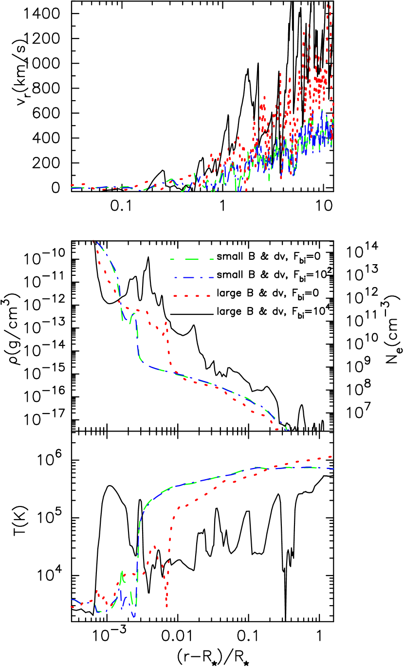
Figure 1: Snapshot structures of the radial velocity, density, and temperature for the different beam energy fluxes at 142 minutes after the electron beam is switched on. The green dashed and blue dash-dotted curves are the results of $F_{bi}=0$ and $10^{2}$erg cm ^-2s^-1 for $B_{*}=1$ G, whereas the red dotted and black solid curves are the results of $F_{bi}=0$ and $10^{4}$ erg cm^-2s^-1 for $B_{*}=5$ G. Note that the vertical scale of the radial velociy is different from that of the density and temperature.

We assume that the electron beam initially streams freely along the flux tube at a constant $v_{b}$. As they approach the parent star, the beam particles start to interact with the dense background ions through Coulomb collisions and become more concentrated due to the flux-tube convergence (see the next subsection). The collisions lead to the heating of surrounding plasma. The heating becomes efficient when the mean free path of the beam is comparable to the local density scale height $H_{\rho}$. The mean free path of an electron colliding with a pool of thermal ions is given by $l_{\rm mfp}\approx 3\times 10^{4}{\rm km}\left(\frac{v_{b}}{3\times 10^{4}{\rm km\;s^{-1}}}\right)^{4}\left(\frac{n}{10^{9}{\rm cm^{-3}}}\right)^{-1}$ (Braginskii, 1965), where $n=10^{9}$cm^-3 is the typical density at the upper transition region or the lower corona (e.g. see SI05, or refer to the density profile in Figure 1 to be discussed in §3). Roughly speaking, for $v_{b}=3\times 10^{4}$ km/s, $l_{\rm mfp}\lesssim H_{\rho}$ when $n>10^{9}$cm^-3. Therefore, we anticipate the inward-propagating electron beam to heat up ambient media from the lower corona to the upper chromosphere. This allows us to assume that the incoming electron beam starts dissipating from $r_{\rm max}=1.1R_{\odot}$ (lower corona) to $r_{\rm min}=1.001R_{\odot}$ (upper chromosphere).

We model the energy flux of the beam to decrease inwardly according to

$$F_{\rm b}\propto\left(\frac{r-r_{\rm min}}{r_{\rm max}-r_{\rm min}}\right)^{k},$$ (5)

where $k$ is a parameter that describes the spacial distribution of the heating. $k=1$ corresponds to constant volumetric heating; namely, the heating rate per unit mass is higher in the upper region (i.e. corona) than in the lower region (i.e. chromosphere). If $k=0.1$, the heating rate per unit mass is more uniformly distributed. In this work, we adopt $k=0.1$ to resemble the situation of a constant beam-heating rate per unit mass. We also assume that the momentum flux of the beam $P_{b}$ dissipates in the same manner as that described by eq. (5) for the energy flux. This implies that although the beam velocity $v_{b}$ does not decay in our dissipation model, the beam density $\rho_{b}$ declines, meaning that more and more beam electrons have been transformed into thermal electrons as the beam progresses downwards in the dissipation region.

The beam heating at the footpoint of one open field line occurs when the planet’s magnetosphere is crossing the field line. Hence, by means of eq. (1), the beam heating proceeds on the timescale

$$t_{beam}={2R_{mp}\over v}\approx 80\,{\rm mins}\left({R_{p}\over R_{J}}\right)\left({v\over 138\,{\rm km/s}}\right)^{-1}\left[\left({B_{p}\over 1\,{\rm G}}\right)\left({B_{*}\over 1\,{\rm G}}\right)^{-1}\left({a\over 10R_{\odot}}\right)^{2}\left({R_{*}\over R_{\odot}}\right)^{-2}\right]^{1/3}.$$ (6)

2.2 Stellar Atmosphere Model

The stellar atmosphere model is based on the 1-D magnetohydrodynamic simulation with radiative cooling and thermal conduction in an open flux tube (SI05). In the original simulation, the heating is given by the nonlinear dissipation of the Alfvén waves excited by the granulations at the photosphere. In the case of $B_{*}=1$ G, we set a rms average amplitude $<dv_{\perp}>\sim 1.8$ km/s at the photosphere, which is estimated from the scaling with the surface convective flux (Suzuki 2007) from the Sun (SI05). In the case of the stronger field $B_{*}=5$ G, the larger rms velocity fluctuation $<dv_{\perp}>\sim 3.6$ km/s is used for the experiment, which is twice the value for the $B_{*}=1$ G case. We neglect the effect of rotation for simplicity in order to focus mainly on the energetics influenced by the electron beam.

When an inward-propagating electron beam described in the above subsection is taken into account, the momentum and energy equations in a 1-D open flux tube are modified to (cf. SI05)

$$\rho\frac{dv_{r}}{dt}=-\frac{\partial p}{\partial r}-\frac{1}{8\pi r^{2}f}\frac{\partial}{\partial r}(r^{2}fB_{\perp}^{2})+\frac{\rho v_{\perp}^{2}}{2r^{2}f}\frac{\partial}{\partial r}(r^{2}f)-\rho\frac{GM_{*}}{r^{2}}-\frac{\partial P_{\rm b}}{\partial r},$$ (7)

and

$$\rho\frac{d}{dt}(e+\frac{v^{2}}{2}+\frac{B^{2}}{8\pi\rho}-\frac{GM_{*}}{r})+\frac{1}{r^{2}f}\frac{\partial}{\partial r}[r^{2}f\{(p+\frac{B^{2}}{8\pi})v_{r}-\frac{B_{r}}{4\pi}(\mbox{\boldmath${B\cdot v}$})\}]$$

$$+\frac{1}{r^{2}f}\frac{\partial}{\partial r}(r^{2}fF_{\rm c})+\frac{1}{r^{2}f}\frac{\partial}{\partial r}(r^{2}fF_{\rm b})+q_{\rm R}=0,$$ (8)

where $\rho$, ${v}$, $p$, $e$, and ${B}$ are the density, velocity, pressure, specific internal energy, and magnetic field strength, respectively; the subscripts $r$ and $\perp$ denote radial and tangential components, respectively; $d/dt$ and $\partial/\partial t$ denote Lagrangian and Eulerian derivatives, respectively; $G$ and $M_{*}$ are the gravitational constant and the stellar mass, respectively; $F_{c}$ is thermal conductive flux; $q_{R}$ is the radiative cooling and $f$ is a super-radial expansion factor. We assume that the super-radial expansion (in addition to the radial expansion $\propto r^{2}$) is a factor of 240 and 480 from the photosphere to $\approx 2R_{\odot}$ in the cases of $B_{*}=1$ and 5 G, respectively. It then follows that to give $B_{*}=$ 1G and 5G, the radial magnetic field strength at the footpoint of the flux tube at the photosphere $B_{ph}$ is 240G and 2400G, respectively.

Note that on account of the convergence of the flux tube toward the central star, the energy flux of the incoming electron beam increases due to the areal focusing. In the case of $B_{*}=1$G, the flux tube converges by a factor of $\approx$14,600 (a factor of $\approx 61$ from the radial convergence and another factor of 240 from the super-radial convergence) from $7.8R_{*}$ (the planet’s orbit) to $1R_{*}$. On the other hand, the converging factor of the flux tube in the $B_{*}=5G$ case is twice as large. In the absence of dissipation, the energy flux of the beam increases by the same factor as the converging factor of the flux tube. In contrast, the same enhancement effect of the electron beam pressure on stellar thermal ions is almost negligible in our calculations because of the small mass of an electron.

3 Results of the Numerical Experiment

We conduct the numerical experiment to study the effects on the stellar atmosphere due to the electron beam with the initial energy fluxes for the two $B_{*}$ cases as described in the preceding session. The experiment is first carried out in the absence of the beam until the simulated atmosphere attains a quasi-steady state. The beam heating is then added afterwards.

Figure 1 shows the snapshot structures of the stellar atmosphere for $B_{*}=$ 1 and 5 G denoted respectively by “small” and “large $B$ and $dv$”, and compares the results with and without the electron-beam injection. In the $B_{*}=1$G case, the results for $F_{bi}=10^{2}$ erg cm^-2 s^-1 (blue curves) are almost identical to those for the no-beam case (green curves). In contrast, the atmospheric structures change noticeably in the larger $B_{*}$ ($=5$G) and $<dv_{\perp}>$ ($=3.6$ km/s) cases, as illustrated by the red and black curves. In the absence of the beam heating, the stronger dissipation arising from the larger $<dv_{\perp}>$ raises the chromospheric temperature and therefore causes the chromosphere to evaporate and expand (see the red curve in the middle panel). The local density scale height increases and the density drops more slowly with $r$. Therefore, the locations of the transition region lie at higher altitudes in the larger $<dv_{\perp}>$ case. A hot and dense region forms in the chromosphere, which we term as “a warm region” (i.e. $T>10^{4}$K, see the bottom panel). It then becomes difficult to further heat up the warm region to the coronal temperature (i.e. $\gtrsim 10^{6}$ K) as a result of the efficient radiative cooling at $T\lesssim 10^{5}$ K (Landini & Monsignori-Fossi, 1990). However, when the beam energy of $F_{bi}=10^{4}$ erg cm^-2 s^-1 is added, the chromosphere is further heated up and thus an even larger warm region can form at the location of $r=1.001-1.01R_{*}$ (see the black curve in the bottom panel). The black curve in the middle panel indicates that the density is on the average much higher in the beam-heated region. Consequently, the heating rate per unit mass becomes smaller and the temperature of the coronal region at $r\gtrsim 1.01R_{*}$ then becomes lower in the case of $F_{bi}=10^{4}$ erg cm^-2 s^-1 than in the case of $F_{bi}=0$ (see the bottom panel). The sharp transition region disappears.

The top panel of Figure 1 shows the radial profile of the stellar wind velocity $v_{r}$. The winds in the outer region ($r\gtrsim 2R_{*}$) are faster in the large $B_{*}$ case. $B_{*}$ equals $B_{ph}/f$, which in fact specifies the flux tube properties. The larger the factor $B_{ph}/f$ is, the more the wave energy dissipates in the outer region of the atmosphere, leading to faster winds (Kojima et al., 2005; Suzuki, 2006). However, the winds on the average are not significantly amplified by the beam heating, as indicated by the large overlap between the red and black curves in the plot. The wind speed at the planet’s orbit is $\approx 300$ km s^-1, which is lower than the Alfvén speeds $\sim 500$ and 1000 km s^-1 there in our cases for $B_{*}=1$ and 5 G. That is, the planet lies inside the Alfvén radius.

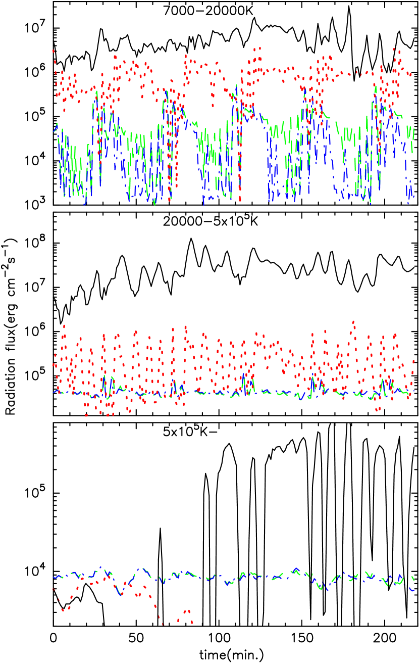
Figure 2: Comparison of the radiative flux arising from different temperature components. The top, middle, and bottom panels show the radiative flux from the gas at the temperatures corresponding to the hot chromosphere, transition region, and corona. The cases for $B_{*}=1$ and 5 G in the absense and presence of the beam heating are plotted with the same color coding as those shown in Figure 1.

Having described the snapshot structures, we should note that the thermal properties of the stellar atmosphere actually fluctuate with time owing to wave propagation and dissipation. As a result, the location and thermal properties of the warm region fluctuate with time as well. Figure 2 shows the evolution of the radiative fluxes arising from different temperature components in the beam and no-beam cases. In general, all of the radiative fluxes fluctuate with time. Nevertheless for the case of $B_{*}=1$G and $<v_{\perp}>=1.8$ km/s, the electron beam of $F_{bi}=10^{2}$ erg cm^-2 s^-1 gives rise to only tiny effects on the radiations compared to the no-beam case, as expected from the snapshot structures shown in Figure 1. In contrast, the case of $F_{bi}=10^{4}$ erg cm^-2 s^-1 corresponding to $B_{*}=5$G exhibits noticeable differences from the no-beam case, which can also be expected from the snapshot structures in Figure 1. The radiative fluxes from the hot chromosphere (7000-20000K) and the transition region (20000-$5\times 10^{5}$K) are greatly enhanced by the warm region in the vicinity of $r=1.001-1.01R_{*}$. Since the warm region is on the average denser than the usual chromosphere and transition region in $r\gtrsim 1.003R_{*}$ (see Figure 1), the radiative flux corresponding to the chromospheric temperature is on average increased by a factor of $\sim 10$ and the radiative flux associated with the transition-region temperature is intensified by a factor of $\sim 100$.

The bottom panel of Figure 2 shows that the beam of $F_{bi}=10^{4}$ erg cm^-2 s^-1 associated with $B_{*}=5$G is able to enhance the radiation from the hot gas of $T>5\times 10^{5}$K occasionally by a factor of $\gtrsim 100$. This radiation is mainly from the warm region that intermittently develops around $r=1.001-1.003R_{*}$. With this beam heating, the temperature of the warm region can sometimes go up and down between $10^{5}$K and $10^{6}$K. This temperature variability is due to the thermal instability (Landini & Monsignori-Fossi, 1990; Suzuki, 2007). The electron beam is energetic enough to continuously heat up the warm region, while the wave dissipation heats it up in a stochastic manner. A small change of the wave heating rate triggers violent fluctuations of temperature in the thermally unstable regime of $10^{5}<T<10^{6}$K.

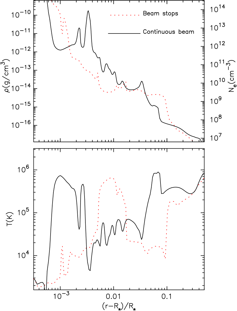
Figure 3: Comparison of snapshot structures of the density and the temperature at $t=219$ minutes for the case with the continuous beam of the energy flux $F_{\rm bi}=10^{4}$erg cm^-2 s^-1 (black solid curve) and the case with the beam switched off at 109 minutes (red dotted curve).

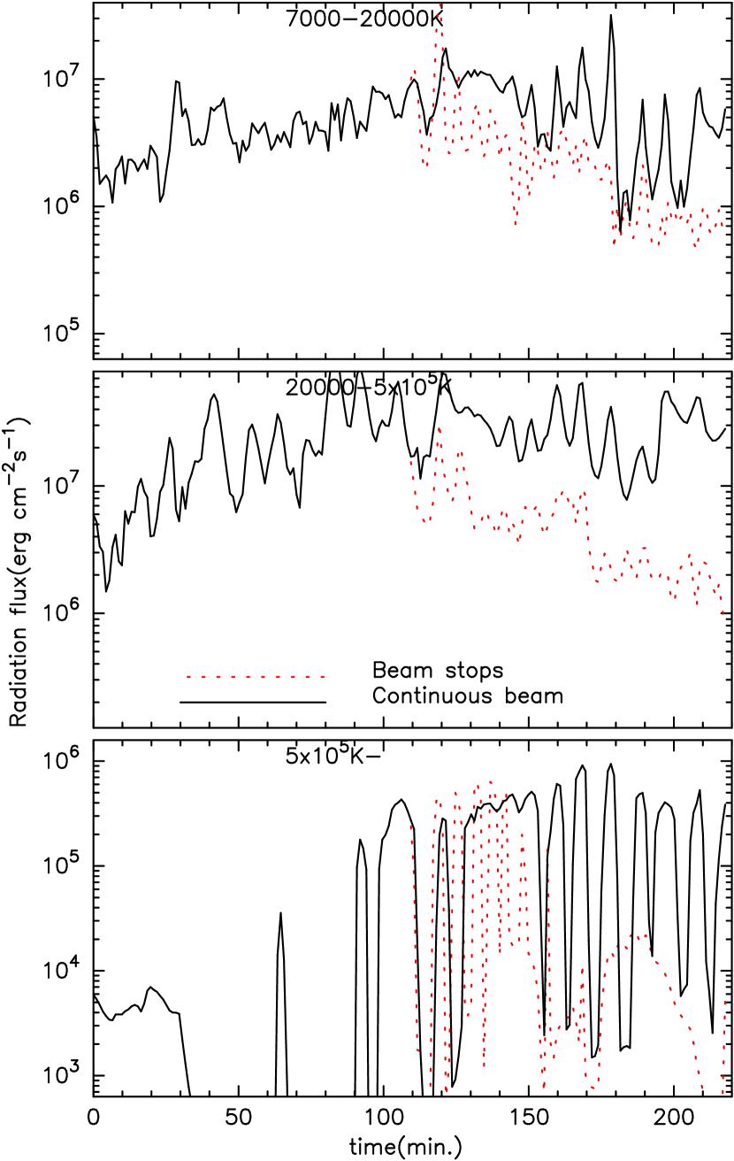
Figure 4: Comparison of the radiative flux for the case with the continuous beam (solid) and the case with the beam switched off at 109 minutes (red dotted). The three panels show the radiation from the gas at the temperatures corresponding to hot chromosphere (top), transition region (middle), and corona (bottom).

As is shown in Figure 2, the thermal response of the stellar atmosphere to the onset of the beam-heating to evolve to the hot state is nearly instantaneously. In §2.1, we estimated the duration of the electron beam as $\sim 100$ min, which is rather short in comparison with the simulation time presented in Figure 2. To estimate the area of the hot spot, it is equally important to examine how long the hot atmosphere can be sustained after the electron beam passes by. Figures 3 & 4 show the results for the $B_{*}=5$G case but the beam is switched off at $t=109$ min. Figure 3, which presents the snapshot structure at $219$ min, namely 110 min after the beam stops, illustrates that while the warm region in the chromosphere is still present as shown by the temperature profile, its density has dropped to the original lower-density level. Figure 4 shows that the radiative fluxes from the hot chromosphere (top) and transition regions (middle) have declined for $\approx$ 50-60 minutes since the beam is switched off, which indicates that the atmosphere takes only a fraction of the heating time to revert to the normal state in the absence of the electron beam. Therefore, the size of the hot spot estimated in terms of the projected area of the planet’s magnetosphere along a flux tube onto the chromosphere is a reasonable approximation.

Shkolnik et al. (2005, 2008) found that in the case of HD 179949, the planet induced Ca II flux averaged over the stellar disk is $\sim 1.5\times 10^{5}$ ergs cm^-2 s^-1, which amounts to an increase of a factor of about 1.04 compared to the non-planet induced Ca II emissions. Hence the Ca II emissions with no planet induced component is $\sim 1.5/0.04\times 10^{5}=3.7\times 10^{6}$ erg cm^-2 s^-1, which is on the similar order of the value given from the model shown by the red-dotted line in Figure 2. In this sense, the model for $B_{*}=5$G and $<dv_{\perp}>=3.6$ km/s may mimic a chromospheric condition similar to that of HD 179949, although our cooling function $q_{R}$ for the chromospheric radiation is based on the observation of the Sun (Anderson & Athay, 1989). Having obtained the radiative flux $\sim 10^{6-7}$ erg cm^-2 s^-1 from the hot chromosphere in the case for $B_{*}=5$G and $<dv_{\perp}>=3.6$ km/s, we can estimate the luminosity of the hot spot. In our model, the cross-sectional area of the converging flux tube in the chromosphere is about 8000 times smaller than the planet’s magnetosphere. In other words, the area of the hot spot in the chromosphere is given by

$$A_{chromo}\approx 10^{17-18}\left({R_{mp}\over 5R_{J}}\right)^{2}\,{\rm cm^{2}},$$ (9)

which when multiplied by the chromospheric flux gives the luminosity of the chromospheric hot spot $\approx 10^{23-25}$ erg/s. This total chromospheric emission is still 2-4 orders of magnitude weaker than the observational Ca II emissions for HD 179949.

4 Summary and Discussions

By conducting a numerical experiment, we study the thermal response of the atmosphere of a solar-type star to the dissipation of an injected electron beam at the coronal base. The experiment is carried out based on the framework of the 1-D magnetohydrodynamic simulation by SI05 with non-linear wave dissipation, radiative cooling, and thermal conduction. We assume that the magnetic stress due to the orbital motion of the planet relative to the stellar coronal fields generates an electron beam, which in turn funnels along the stellar open field lines to the central star. As the beam travels inwards, the energy flux of the incoming electron beam is intensified by the areal focusing of the super-radially converging open flux tube.

We use the stellar parameters of HD 179949 as an illustrative example but ignore possible magnetic properties arising from its stellar rotation. When the average stellar field at the photosphere $B_{*}$ is about 1 G and the average amplitude of the wave velocity $<v_{\perp}>$ is about 1.8 km/s, the stellar atmosphere is not considerably altered after the beam dissipation is turned on. In contrast, when $B_{*}=$5 G and $<v_{\perp}>=3.6$ km/s, we find that a warm region forms in the chromosphere. The warm region becomes substantially hotter and denser once the electron-beam heating is switched on. As a result, the beam-intensified warm region enhances the chromospheric radiative flux by a factor of $\sim 10$, and the radiative flux corresponding to the temperature of the transition region by a factor of $\sim 100$. The warm region can also intermittently contribute to the radiative flux associated with the coronal temperature by a factor of $\sim 100$ due to the thermal instability (Landini & Monsignori-Fossi, 1990). In other words, the planet-induced radiations are not perturbations in the local region of the hot spot compared to the normal state of the stellar emissions. However, owing to the small area of the heating spot, the total luminosity of the beam-induced chromospheric radiation is 2-4 orders of magnitude smaller than the observed Ca II emissions from HD 179949.

The energetics of the planet-induced emissions becomes a more serious problem in our numerical experiments when explaining the statistical results of X-rays from planet-host stars: stars with close-in giant planets are on average more X-ray active by a factor $\sim 4$ than those with planets that are more distant (Kashyap et al., 2008). Since the typical X-ray luminosity from a solar-type stars is $\gtrsim 10^{27-28}$ erg/s, the planet-induced X-ray inferred from the statistical analysis is actually even stronger than the planet-induced Ca II emissions from HD 179949. Our simulation results show that an $\sim 100$ times enhancement in X-ray due occasionally to the thermal instability of the small warm region contributes only an even more negligible perturbation to the total X-ray emission, rather than being comparable to it.

We note that our open-field model for the chromospheric emissions is different from those occurring on the Sun where the emissions come primarily from the solar plage regions in closed magnetic loops. Needless to say, our 1-D numerical experiment restricts ourselves to exclude any mechanical and thermal influence of the heating area on neighboring open fields and closed magnetic loops. As such, our results leave an open question as to whether the thermal instability or any other magnetic instabilities (e.g. Lanza 2008; Ishikawa et al. 2008) can be further triggered around the beam-heated spot to liberate more energy.

In our numerical experiment $B_{*}$ has been taken to be 1 and 5 G, which is consistent with the field measurements via spectrapolarimetry for the similar spectral type dwarf $\tau$ Bootis (Catala et al., 2007). However, the field strength inferred from the Stokes V observation may be underestimated due to the cancellation of circular polarization arising from the opposite directions of $B_{*}$ along the line of sight. It is normally expected that a faster rotator and therefore a stronger X-ray emitter may possess stronger $B_{*}$ than the Sun (Rüedi et al., 1997; Güdel, 2007). For instance, $B_{*}$ of HD 179949 has been assumed to be $\approx$ 8-9$\times$ solar value by scaling with the X-ray flux (Saar et al., 2004). Furthermore, Montesinos & Jordan (1993) related $B_{*}$ and the filling factor $f_{s}$ to the Rossby number $Ro$ ($\equiv P_{rot}/\tau_{c}$, where $P_{rot}$ is the rotation period and $\tau_{c}$ is the convection turnover time) of a dwarf star. In the case of HD 179949, $P_{rot}$ has been suggested to be about 7 days (Wolf & Harmanec, 2004; Shkolnik et al., 2008) and $\tau_{c}\approx 4.287$ days may be inferred from its color B$-$V=0.503 (Noyes et al. 1984). Thus following Montesinos & Jordan (1993), we obtain the average field $Bf_{s}=37.6$ G and the filling factor $f_{s}=0.02$. If we assume that these magnetic properties are contributed mainly from the open-field region of our model, then $Bf_{s}=37.6$ G is equivalent to $B_{*}$ and the filling factor $f_{s}=0.02$ may correspond to the super-radial expansion factor $1/f$ in our experiment. In reality, some of the contribution may come from closed-field regions (Montesinos & Jordan, 1993), which introduces additional complexity.

The other free parameter that governs our numerical results is the power spectrum of MHD waves. The stellar macroturbulent velocity $v_{mac}$ for HD 179949 is expected to be 2 times larger than that for the Sun (Saar & Osten, 1997; Saar et al., 2004). In our experiment, we adopt a larger $<dv_{\perp}>$ for the stronger $B_{*}$ case. However, the correlation between $v_{mac}$ and $<dv_{\perp}>$ is not tested in this work and how these velocities are associated with $B_{*}$ is not modelled in our numerical experiment. After all, in view of all of the uncertainties and complexities mentioned above, our results serve only as the fiducial examples for future studies. The numerical experiment covering a broader parameter space coupled with more magnetic-field measurements will be essential to further diagnose the problem.

The effect of the centrifugal force is not implemented in the present numerical experiment. While it is a reasonable approximation for thermally driven winds from a slow rotator like the Sun, the magneto-centrifugal winds play an equally important role in accelerating stellar winds for a star rotating $\sim 10$ times faster than the Sun (Belcher & MacGregor, 1976; Washimi & Shibata, 1993; Preusse et al., 2006). The centrifugal force of a 7 day-period star is $\sim 1/5$ that of a 3 day-period star, as the force is proportional to the square of the rotation frequency. The effect of the centrifugal force on the stellar atmosphere will be investigated in a future work.

While most of the previous magnetohydrodynamic simulations and studies have focused on the planet’s side for the magnetic interactions (Ip et al. 2004; Preusse et al. 2006, 2007; cf. Laine et al. 2008 for a young hot Jupiter), our numerical experiment makes an attempt to investigate how a stellar atmosphere down to the photosphere in the open field region responds to the dissipation likely from a hot Jupiter. The current model is simplified in such a way that we prescribe the energy dissipation and ignore stellar rotation. Nevertheless, the dissipation contributed by the planet is described only by the energy flux $F_{b}$ at the coronal base, meaning that $F_{b}$ is not necessarily specific only to an incoming electron beam but can be in the form of other dissipative sources (e.g. damping of Alfv́en waves) with proper modification. Furthermore, our simulation lays the framework to extend the calculations for other types of dwarf stars if the corresponding magnetic wave amplitudes and power spectra are specified.

References

- Anderson & Athay (1989) Anderson, L. S., & Athay, R. G. 1989, ApJ, 346, 1010
- Braginskii (1965) Braginskii, S. I. 1965, Rev. Plasma Phys., 1, 205
- Belcher & MacGregor (1976) Belcher, J. W., & MacGregor, K. B. 1976, ApJ, 210, 496
- Butler et al. (2006) Butler, R. P., Wright, J. T., Marcy, G. W., Fischer, D. A., Vogt, S. S., Tinney, C. G., Jones, H. R. A., Carter, B. D., Johnson, J. A., McCarthy, C., & Penny, A. J. 2006, ApJ, 646, 505
- Catala et al. (2007) Catala, C., Donati, J.-F., Shkolnik, E., Bohlender, D., & Alecian, E. 2007, MNRAS, 374, L42
- Cuntz et al. (2000) Cuntz, M., Saar, S. H., & Musielak, Z. E. 2000, ApJ, 533, L151
- Gu et al. (2005) Gu, P.-G., Shkolnik, E., Li, S.-L., & Liu, X.-W. 2005, Astronomische Nachrichten, 326, 909
- Güdel (2007) Güdel, M. 2007, Living Rev. Solar Phys., 4, 3
- Ip et al. (2004) Ip, W.-H., Kopp, A., & Hu, J.-H. 2004, ApJ, 602, L53
- Ishikawa et al. (2008) Ishikawa, R., Tsuneta, S., Ichimoto, K., Isobe, H., Katsukawa, Y., Lites, B. W., Nagata, S., Shimizu, T., Shine, R. A., Suematsu, Y., Tarbell, T. D., & Title, A. M. 2008, A&A, 481, L25
- Jackson et al. (2009) Jackson, B., Barnes, R., & Greenberg, R. 2009, ApJ, 698, 1357
- Jacques (1977) Jacques, S. A. 1977, ApJ, 215, 942
- Kashyap et al. (2008) Kashyap, V. L., Drake, J. J., & Saar, S. H. 2008, ApJ, 687, 1339
- Kojima et al. (2005) Kojima, M., Fujiki, K., Hirano, M., Tokumaru, M., Ohmi, T., and Hakamada K., 2005, ”The Sun and the heliosphere as an Integrated System”, G. Poletto and S. T. Suess, Eds. Kluwer Academic Publishers, 147
- Kopp & Holzer (1976) Kopp, R. A., & Holzer, T. E. 1976, Sol. Phys., 49, 43
- Laine et al. (2008) Laine, R. O., Lin, D. N. C., & Dong, S.-F. 2008, ApJ, 685, 521
- Landini & Monsignori-Fossi (1990) Landini, M., & Monsignori-Fossi, B. C. 1990, A&AS, 82, 229
- Lanza (2008) Lanza, A. F. 2008, A&A, 487, 1163
- Lin et al. (1996) Lin, D. N. C., Bodenheimer, P., & Richardson, D. C. 1996, Nature, 380, 606
- Montesinos & Jordan (1993) Montesinos, B., Jordan, C. 1993, MNRAS, 264, 900
- Noyes et al. (1984) Noyes, R. W., Hartmann, L. W., Baliunas, S. L., Duncan, D. K., Vaughan, A. H. 1984, ApJ, 279, 763
- Pfahl et al. (2008) Pfahl, E., Arras, P., & Paxton, B. 2008, ApJ, 679, 783
- Preusse et al. (2005) Preusse, S., Kopp, A., Büchner, J., & Motschmann, U. 2005, A&A, 434, 1191
- Preusse et al. (2006) Preusse, S., Kopp, A., Büchner, J., & Motschmann, U. 2006, A&A, 460, 317
- Preusse et al. (2007) Preusse, S., Kopp, A., Büchner, J., & Motschmann, U. 2007, Planetary & Space Science, 55, 589
- Rubenstein & Schaefer (2000) Rubenstein, E. P. & Schaefer, B. E. 2000, ApJ, 529, 1031
- Rüedi et al. (1997) Rüedi, I, Solanki, S. K., Mathys, G., & Saar, S. H. 1997, A&A, 318, 429
- Saar & Osten (1997) Saar, S. H., & Osten, R. A. 1997, MNRAS, 284, 803
- Saar et al. (2004) Saar, S. H., Cuntz, M. & Shkolnik, E. 2004, IAU Symposium, Stars as Suns: Activity, Evolution, and Planets, A. K. Dupree and A. O. Benz, Eds, 219, 355
- Shkolnik et al. (2003) Shkolnik, E., Walker, G. A.H., & Bohlender, D. A., 2003, ApJ, 597, 1092
- Shkolnik et al. (2005) Shkolnik, E., Walker, G. A.H., Bohlender, D. A., Gu, P.-G., & Kürster, M. 2005, ApJ, 622, 1075
- Shkolnik et al. (2008) Shkolnik, E., Bohlender, D. A., Walker, G. A. H., & Collier Cameron, A. 2008, ApJ, 676, 628
- Suzuki & Inutsuka (2005) Suzuki, T. K. & Inutsuka, S.-I. 2005, ApJ, 632, L49 (SI05)
- Suzuki (2006) Suzuki, T. K. 2006, ApJ, 640, L75
- Suzuki & Inutsuka (2006) Suzuki, T. K. & Inutsuka, S.-I. 2006, Journal of Geophysical Research, l11, A06101
- Suzuki (2007) Suzuki, T. K. 2007, ApJ, 659, 1592
- Tsuneta et al. (2008) Tsuneta, S., Ichimoto, K., Katsukawa, Y., Lites, B. W., Matsuzaki, K., Nagata, S., Orozco Suarez, D., Shimizu, T., Shimojo, M., Shine, R. A., Suematsu, Y., Suzuki, T. K., Tarbell, T. D., & Title, A. M. 2008, ApJ, 688, 1374
- Walker et al. (2008) Walker, G. A. H. et al. 2008, A&A, 482, 691
- Washimi & Shibata (1993) Washimi, & Shibata 1993, MNRAS, 262, 936
- Wolf & Harmanec (2004) Wolf, M. & Harmanec, P. 2004, Inf. Bull. Variable Stars, 5575, 1
- Zarka (2001) Zarka, P., Treumann, R. A., Ryabov, B. P., & Ryabov, V. B. 2001, Ap&SS, 277, 293
- Zarka (2007) Zarka, P. 2007, Plan. Spa. Sci., 55, 589