Theory of Raman and Resonant Inelastic X-ray Scattering from Collective Orbital Excitations in YTiO₃

Abstract

We present two different theories for Raman scattering and Resonant Inelastic X-ray Scattering (RIXS) in the low temperature ferromagnetic phase of YTiO₃ and compare this to the available experimental data. For description of the orbital ground-state and orbital excitations, we consider two models corresponding to two theoretical limits: one where the $t_{2g}$ orbitals are degenerate, and the other where strong lattice distortions split them. In the former model the orbitals interact through superexchange. The resulting superexchange Hamiltonian yields an orbitally ordered ground state with collective orbital excitations on top of it – the orbitons. In the orbital-lattice model, on the other hand, distortions lead to local $dd$-transitions between crystal field levels. Correspondingly, the orbital response functions that determine Raman and RIXS lineshapes and intensities are of cooperative or single-ion character. We find that the superexchange model yields theoretical Raman and RIXS spectra that fit very well to the experimental data.

I Introduction

In many 3$d$ transition metal compounds, like the titanates and colossal magnetoresistance manganites, the low-energy orbital degrees of freedom are (approximately) degenerate. This leads to all kinds of interesting phenomena like cooperative Jahn-Teller (JT) distortions, orbital frustration and strong spin-orbit coupling. Orbitals on neighboring orbitally active ions can be coupled via JT-distortions and via superexchangeGehring1975 ; Kugel1982 ; Goodenough1963 . Both couplings can give rise to an orbitally ordered ground state. However, the nature of the orbital excitations on top of the orbitally ordered ground state is very different depending on the coupling mechanism. In a pure superexchange system, collective excitations called ‘orbitons’ emerge. These collective orbital excitations are coherent waves of excited orbitals, similar to the spin wave excitations in spin systems. When this system is coupled to the lattice, as is the case when JT-distortions are present, interaction with phonons destroys the orbiton coherence. The distortions lift the orbital degeneracy and the excitations become local $dd$-excitations.

The titanates, with a pseudo-cubic perovskite lattice structure, are good candidates to support orbitons. The Ti ions with their 3$d^{1}$ configuration have one electron in one of the three nearly degenerate $t_{2g}$ orbitals. Since these orbitals are directed away from the neighboring oxygen ions, the coupling to the lattice is expected to be small. Further, it has been shownKhaliullin2002 ; Khaliullin2003 that a superexchange-only model explains many of the ground state properties of YTiO₃. Also, there is experimental evidence that LaTiO₃ is a (superexchange-driven) orbital liquidKeimer2000 ; Khaliullin2000 ; Cheng2008 . On the other hand, local crystal field models also well reproduce some of the physical properties of the titanatesMochizuki2003 ; Pavarini2004 ; Pavarini2005 ; Cwik2003 ; Schmitz2005 ; Haverkort2005 ; Solovyev2006 ; Akimitsu2001 ; Kiyama2003 ; Kubota2004 ; Kiyama2005 . Both models have their shortcomings as well: a Jahn-Teller dominated description is not able to reproduce the spin wave spectrum, which is nearly isotropic in both spin and real space, while the superexchange model has difficulties explaining the experimentally observed orbital polarizationAkimitsu2001 ; Kiyama2003 ; Kubota2004 ; Kiyama2005 . Consequently, it still remains controversial which mechanism dominates the orbitals in titanatesKhaliullin2005 .

In order to resolve this controversy, it is of crucial importance to compare recent Raman and Resonant Inelastic X-ray Scattering (RIXS) experiments on titanatesUlrich2006 ; Ulrich2008 ; experimentalpaper to both of the competing theories.

The experimental observation of orbitons is a difficult task, as is underscored by the heavily debated Raman measurements on LaMnO₃Saitoh2001 ; Grueninger2002 ; Saitoh2002 . Because the hallmark of collective excitations is dispersion, a much better technique to directly probe orbitons is RIXS. With its energy resolution drastically improved over the last few years, RIXS now offers a whole new way of accessing the elementary excitations of solids, complementary to for instance Raman and neutron scattering. In this paper we analyze recent Raman and RIXS spectraUlrich2006 ; Ulrich2008 ; experimentalpaper for YTiO₃ from the point of view of a superexchange-only model and the alternative extreme of a completely local, lattice distortion dominated model. We find that while the orbital-lattice model can be finetuned to capture some aspects of the observed spectra, the collective superexchange model yields a much better overall description of the Raman and RIXS data.

The paper is organized as follows: Sec. II compactly reviews previous work on YTiO₃ and introduces the superexchange formalism and the local crystal field model. Sections III and IV deal with the theory of Raman scattering and RIXS respectively, in both the superexchange and crystal field models.

II Two models of YTiO₃

For the existence of collective excitations of orbitals, the so-called orbitons, it makes a difference whether the orbital order is driven by JT distortions or superexchangeGehring1975 ; Kugel1982 . For large JT distortions, the crystal field splitting is large and a local picture applies: the collective nature of the orbital excitations characteristic of orbitons is lost. In materials where the orbital-lattice coupling is small, the superexchange interactions between orbitals can dominate over crystal field splittings due to lattice distortions. The Ti ions have a 3$d^{1}$ configuration, and the octahedral crystal field induces a splitting between the higher energy $e_{g}$ and lower energy $t_{2g}$ levels. Because the $t_{2g}$ orbitals are not directed towards neighboring oxygen ions, they are not expected to couple strongly to lattice distortions.

Building on this assumption, one can derive a superexchange Hamiltonian starting from a Hubbard model. Below, we follow Refs. [Khaliullin2002, ; Khaliullin2003, ] closely. By symmetry, the hopping term connects, for instance, the $zx$ to $zx$ and $yz$ to $yz$ orbitals along the $z$-direction ($c$-axis) via the intermediate oxygen 2$p_{\pi}$ states. $xy$ orbitals are not coupled along this direction. In the limit of large on-site Coulomb repulsion $U$, this leads to a superexchange interaction that depends on the spatial direction of a bond, and the resulting model is intrinsically frustrated: on any given ion, there is no orbital that minimizes the bond energy in all directions simultaneously.

Because YTiO₃ is ferromagnetic at low temperatureGoral1982 ($T_{c}\approx 30$ K), we restrict ourselves to the completely ferromagnetic part of the Hilbert space. Then one obtains the simple Hamiltonian

$$\hat{H}_{0}=\frac{1}{2}J_{\rm orb}\sum_{\left<i,j\right>}\left(\hat{A}^{(\gamma)}_{ij}+\frac{n_{\gamma,i}+n_{\gamma,j}}{2}\right),$$ (1)

with the orbital exchange integral $J_{\rm orb}=r_{1}J_{SE}$, where $r_{1}=1/(1-3J_{H}/U)\approx 1.56$ parametrizing Hund’s rule coupling and $J_{SE}=4t^{2}/U$ is the superexchange constant derived from the Hubbard model. The operator $\hat{A}^{(\gamma)}_{ij}$ depends on the direction $\gamma$ of the bond $ij$. For example, in the $z$-direction we have

$$\hat{A}^{(c)}_{ij}=n_{a,i}n_{a,j}+n_{b,i}n_{b,j}+a^{{\dagger}}_{i}b^{\phantom{{\dagger}}}_{i}b^{{\dagger}}_{j}a^{\phantom{{\dagger}}}_{j}+b^{{\dagger}}_{i}a^{\phantom{{\dagger}}}_{i}a^{{\dagger}}_{j}b^{\phantom{{\dagger}}}_{j}.$$ (2)

The operators $a^{{\dagger}},b^{{\dagger}}$ and $c^{{\dagger}}$ create an electron in the $yz$-, $zx$- and $xy$-orbital, respectively, and $n_{a}=a^{{\dagger}}a$. The Hamiltonian can also be written in terms of interacting effective angular momenta $l=1$, operating on the $t_{2g}$ triplet. Because of the orbital frustration, these can form a myriad of different classical ground states. Refs. [Khaliullin2002, , Khaliullin2003, ] conclude that a $4$-sublattice quadrupole ordered state is favored, in which the orbitals

$$\left|\psi_{c}\right>=\frac{1}{\sqrt{3}}\left(\left|d_{yz}\right>\pm\left|d_{zx}\right>\pm\left|d_{xy}\right>\right)$$ (3)

are condensed. The signs $\pm$ alternate between the sublattices, such that nearest-neighbor orbitals are orthogonal, supporting ferromagnetic order. On top of this condensate, two species of orbitons can be created, loosely speaking by populating either one of the two orbitals orthogonal to $\psi_{c}$. The orbiton spectrum has $3N^{1/3}$ Goldstone modes (where $N$ is the total number of Ti ions), because the number of orbitals of a specific “color” is conserved in the plane in which it is lying. However, in YTiO₃ the TiO₆ octahedra are tilted. Because of this, hopping between different $t_{2g}$ orbitals is now no longer symmetry forbidden, and the conservation of orbital “color” is violated, removing the Goldstone modes. When also some anharmonic terms of the Hamiltonian are taken into account on a mean field level, the orbiton dispersion becomesKhaliullin2003

$$\omega_{1/2,{\bf k}}= \sqrt{Z_{\varepsilon}Z_{f}}J_{\rm orb}\{1-(1-2\varepsilon)(1-2f)(\gamma_{1,{\bf k}}\pm\kappa_{\bf k})^{2}$$

$$-2(\varepsilon-f)(\gamma_{1,{\bf k}}\pm\kappa_{\bf k})\}^{1/2},$$ (4)

where we use the signs $+$ and $-$ for $\omega_{1,{\bf k}}$ and $\omega_{2,{\bf k}}$ respectively. Further, $\sqrt{Z_{\varepsilon}Z_{f}}\approx 1.96$, $f\approx 0.086$, $\varepsilon\approx 0.18$, $\gamma_{1,{\bf k}}=(c_{x}+c_{y}+c_{z})/3$ and $\kappa_{\bf k}=\sqrt{\gamma^{2}_{2,{\bf k}}+\gamma^{2}_{2,{\bf k}}}$ with $\gamma_{2,{\bf k}}=\sqrt{3}(c_{y}-c_{x})/6$ and $\gamma_{3,{\bf k}}=(2c_{z}-c_{x}-c_{y})/6$ with $c_{\alpha}=\cos k_{\alpha}$. Eq. (4) describes the collective orbital modes that disperse up to energies of $2J_{\rm orb}$ and have a gap of approximately $J_{\rm orb}$.

In the second orbital model for YTiO₃ that we consider, lattice distortions dominate over superexchange interactions. Pavarini et al.Pavarini2004 ; Pavarini2005 did a DMFT+LDA calculation and found that lattice distortions of the GdFeO₃-type lift the orbital degeneracy. They also obtained four sublattices. The resulting local eigenstates of the $t_{2g}$ system arePavarini2005

$$\left|1\right> =0.781\left|yz\right>-0.073\left|zx\right>+0.620\left|xy\right>$$ (5)

$$\left|2\right> =-0.571\left|yz\right>+0.319\left|zx\right>+0.757\left|xy\right>$$ (6)

$$\left|3\right> =0.253\left|yz\right>+0.945\left|zx\right>-0.207\left|xy\right>$$ (7)

for sublattice 1, with corresponding orbital energies $\epsilon_{1}=289$ meV, $\epsilon_{2}=488$ meV and $\epsilon_{3}=620$ meV. This yields excitation energies $\omega_{1}=\epsilon_{2}-\epsilon_{1}=199$ meV, $\omega_{2}=\epsilon_{3}-\epsilon_{1}=331$ meV. The orbital states on the other sublattices can be obtained from lattice symmetry considerationsPavarini2005 . Superexchange processes are treated as a perturbation in this model, broadening the states generated by lattice distortions. This picture is also supported by other theoretical workMizokawa1996 ; Mochizuki2003 ; Schmitz2005 ; Ishihara2004 .

It is possible to rotate the axes on each of the sublattices in such a way that in the new coordinates, the eigenstates are still given by Eqs. (5) through (7):

$${\rm subl.}\;1:(x,y,z) \mapsto(x,y,z)$$ (8)

$${\rm subl.}\;2:(x,y,z) \mapsto(y,x,z)$$ (9)

$${\rm subl.}\;3:(x,y,z) \mapsto(x,y,-z)$$ (10)

$${\rm subl.}\;4:(x,y,z) \mapsto(y,x,-z).$$ (11)

Correspondingly, the orbiton operators transform as follows:

$${\rm subl.}\;1:(a,b,c) \mapsto(a,b,c)$$ (12)

$${\rm subl.}\;2:(a,b,c) \mapsto(b,a,c)$$ (13)

$${\rm subl.}\;3:(a,b,c) \mapsto(-a,-b,c)$$ (14)

$${\rm subl.}\;4:(a,b,c) \mapsto(-b,-a,c).$$ (15)

III Raman scattering

In the search for orbitons, Raman scattering has been an important tool for experimentalists. After the controversial first observation of orbitons in LaMnO₃Saitoh2001 ; Grueninger2002 ; Saitoh2002 , the titanates now seem to be a more promising candidate. In addition to the reasons mentioned in previous sections, recent Raman data by Ulrich et al.Ulrich2006 should be noted, which shows a striking temperature dependence: the spectral weight of the $235$ meV peak in YTiO₃ increases dramatically when temperature is lowered. This can be naturally explained by collective orbitons: as temperature drops, the orbitons gain coherence and the spectral weight increases, analogous to two-magnon Raman scattering in the cupratesKnoll1990 . From the local $dd$-excitation point of view, temperature should not affect the intensity of local transitions between crystal field levels. Also, Ulrich et al. found that the polarization dependence of the spectra is hard to reconcile with the local excitation picture a result that we will reproduce below. In optical dataRueckamp2005 , a peak is seen at the same energy and was ascribed to orbital excitations.

Earlier theoretical work on Raman scattering in the titanatesIshihara2004 built on the assumption that JT-distortions determine the symmetry of the orbital order. In this paper, we investigate the Raman spectrum of YTiO₃ in both the lattice distortion and superexchange frameworks laid out in Sec. II. We start out with the Loudon-Fleury effective Raman scattering operatorElliott1963 ; Fleury1968

$$\hat{R}\propto\sum_{\left<i,j\right>}\left({\boldsymbol{\epsilon}}_{i}\cdot{\boldsymbol{\delta}}_{ij}\right)\left({\boldsymbol{\epsilon}}_{f}\cdot{\boldsymbol{\delta}}_{ij}\right)\left(\hat{A}^{(\gamma)}_{ij}+\frac{n_{\gamma,i}+n_{\gamma,j}}{2}\right)$$ (16)

where the usual spin exchange Hamiltonian has been replaced by the orbital Hamiltonian of Eq. (1). ${\boldsymbol{\epsilon}}_{i,f}$ are the electric field vectors of the in- and out-going light, ${\boldsymbol{\delta}}_{ij}$ connects nearest neighbors $i$ and $j$. The physical picture is that the light induces an electric dipole transition to the intermediate state where a 3$d\;t_{2g}$ electron ends up on a neighboring Ti ion, after which one of the electrons of this now doubly occupied site can hop back in another transition. In this process, the two involved electrons can end up in different orbitals, resulting in a two-orbiton excitation, in full analogy with two-magnon Raman scattering in the cuprates. As the light forces the electrons to perform a superexchange process independently of the intrinsic coupling mechanism of the orbitals, this effective Raman operator holds for the lattice distortion model too.

With this scattering operator, we calculate the Raman spectrum for the superexchange model. Similar calculations have been done before in the context of Raman scattering on orbital excitations in vanadatesMiyasaka2005 . Adopting the geometry used in the experiment of Ref. [Ulrich2006, ], we take the electric field vectors to be in the plane parallel to the $[110]$- and $[001]$-directions: ${\boldsymbol{\epsilon}}_{i(f)}\propto(\frac{1}{\sqrt{2}}\sin\theta_{i(f)},\frac{1}{\sqrt{2}}\sin\theta_{i(f)},\cos\theta_{i(f)})$ where $\theta_{i(f)}$ is the angle the electric field vector makes with the $c$-axis. Throughout this paper we use a coordinate system in which the nearest neighbor Ti-Ti bonds are parallel to the coordinate axes. Substituting into Eq. (16) and using that $\sum_{i}n_{\gamma,i}$ is a conserved quantity in the superexchange model and that $\hat{H}_{0}\left|0\right>\propto\left|0\right>$, we find for inelastic Raman scattering

$$\hat{R}\propto\left(\cos\theta_{i}\cos\theta_{f}-\frac{1}{2}\sin\theta_{i}\sin\theta_{f}\right)\sum_{\left<i,j\right>_{c}}\hat{A}^{(c)}_{ij}$$ (17)

where the sum is over bonds in the $c$-direction only. Performing the transformations mentioned in Sec. II, condensing $\psi_{c}$ and Fourier transforming, we obtain

$$\sum_{\left<i,j\right>_{c}}\hat{A}^{(c)} =\frac{2}{3}\sum_{\bf k}\left[(a^{{\dagger}}_{\bf k}-b^{{\dagger}}_{\bf k})(a^{\phantom{{\dagger}}}_{\bf k}-b^{\phantom{{\dagger}}}_{\bf k})+\frac{c_{z}}{2}(a^{{\dagger}}_{\bf k}-b^{{\dagger}}_{\bf k})\times\right.$$

$$\left.(a^{{\dagger}}_{-{\bf k}}-b^{{\dagger}}_{-{\bf k}})+\frac{c_{z}}{2}(a^{\phantom{{\dagger}}}_{-{\bf k}}-b^{\phantom{{\dagger}}}_{-{\bf k}})(a^{\phantom{{\dagger}}}_{\bf k}-b^{\phantom{{\dagger}}}_{\bf k})\right]$$ (18)

where only quadratic terms in the operators are retained. Linear terms do not appear. Next, this result is Bogoliubov transformed according to

$$a_{\bf k} =u_{\bf k}{\rm ch}\;\theta_{1,{\bf k}}\alpha^{\phantom{{\dagger}}}_{1,{\bf k}}+v_{\bf k}{\rm ch}\;\theta_{2,{\bf k}}\alpha^{\phantom{{\dagger}}}_{2,{\bf k}}$$

$$-u_{\bf k}{\rm sh}\;\theta_{1,{\bf k}}\alpha^{{\dagger}}_{1,-{\bf k}}-v_{\bf k}{\rm sh}\;\theta_{2,{\bf k}}\alpha^{{\dagger}}_{2,-{\bf k}},$$ (19)

$$b_{\bf k} =-v_{\bf k}{\rm ch}\;\theta_{1,{\bf k}}\alpha^{\phantom{{\dagger}}}_{1,{\bf k}}+u_{\bf k}{\rm ch}\;\theta_{2,{\bf k}}\alpha^{\phantom{{\dagger}}}_{2,{\bf k}}$$

$$+v_{\bf k}{\rm sh}\;\theta_{1,{\bf k}}\alpha^{{\dagger}}_{1,-{\bf k}}-u_{\bf k}{\rm sh}\;\theta_{2,{\bf k}}\alpha^{{\dagger}}_{2,-{\bf k}},$$ (20)

where the indices $1,2$ refer to the orbiton branch. This transformation diagonalizes $\hat{H}_{0}$ up to quadratic order if

$$u_{\bf k} =\sqrt{\frac{1}{2}+\frac{\gamma_{2,{\bf k}}}{2\kappa_{\bf k}}}$$ (21)

$$v_{\bf k} ={\rm sign}(\gamma_{3,{\bf k}})\sqrt{\frac{1}{2}-\frac{\gamma_{2,{\bf k}}}{2\kappa_{\bf k}}}$$ (22)

$$\tanh 2\theta_{1(2),{\bf k}} =\gamma_{1,{\bf k}}\pm\kappa_{\bf k}.$$ (23)

The effective Raman scattering operator now either produces two orbitons or scatters single orbitons already present in the initial state. At zero temperature, the initial state has no orbitons (in “linear orbital wave theory”, i.e. if we neglect orbiton-orbiton interactions), so we keep only the two-orbiton creation part of $\sum_{\left<i,j\right>_{c}}\hat{A}^{(c)}$ in Eq. (18):

$$\frac{1}{3} \sum_{\bf k}\left[\left\{(u+v)^{2}(c_{z}{\rm ch}\;2\theta_{1}-{\rm sh}\;2\theta_{1})\right\}\alpha^{{\dagger}}_{1,{\bf k}}\alpha^{{\dagger}}_{1,-{\bf k}}\right.$$

$$+\left\{(u-v)^{2}(c_{z}{\rm ch}\;2\theta_{2}-{\rm sh}\;2\theta_{2})\right\}\alpha^{{\dagger}}_{2,{\bf k}}\alpha^{{\dagger}}_{2,-{\bf k}}$$

$$+2\left\{(u^{2}-v^{2})[{\rm sh}\;(\theta_{1}+\theta_{2})\left.-c_{z}{\rm ch}\;(\theta_{1}+\theta_{2})]\right\}\alpha^{{\dagger}}_{1,{\bf k}}\alpha^{{\dagger}}_{2,-{\bf k}}\right]$$ (24)

where $c_{z}=\cos k_{z}$ and the index ${\bf k}$ is implied on every $u,v,\theta_{1}$ and $\theta_{2}$.

The cross section at zero temperature now is

$$\frac{d^{2}\sigma}{d\omega d\Omega}\propto\sum_{f}\left|\left<f\right|\hat{R}\left|0\right>\right|^{2}\delta(\omega-\omega_{f})$$ (25)

with $f$ labelling the two-orbiton final states with energy $\omega_{f}$. The corresponding matrix elements are given by Eq. (24).

Because there are orbiton-orbiton interaction terms in the Hamiltonian which are neglected in “linear orbital wave theory”, we introduce a phenomenological orbiton damping of $\gamma=30$ meV. Also, broadening from other sources such as interaction with phonons and magnons can be mimicked this way.

The result is displayed in Fig. 1, compared to the data from Ref. [Ulrich2006, ]. In the superexchange model, only two-orbiton creation processes contribute to the Raman spectrum. The best fit is obtained for $J_{\rm orb}=65$ meV, close to the value estimated in Ref. [Khaliullin2003, ] from magnon data of YTiO₃Ulrich2002 . Including orbiton-orbiton interactions will probably reduce the peak energy (in analogy to two-magnon Raman scattering), increasing the fit parameter $J_{SE}$.

The local model of YTiO₃ also yields Raman spectra via Eq. (16). In this model, the orbital order makes the $c$-direction different from the $a$ and $b$ ones. Therefore, all bond directions are considered separately. For technical convenience, the rotations Eqs. (12) through (15) are first performed. Bonds in the $c$-direction connect sublattice $1$ to sublattice $3$, and $2$ to $4$. Both these bonds give the same contribution to the Raman operator:

$$\sum_{\left<i,j\right>_{c}} \left(\hat{A}^{(c)}_{ij}+\frac{1}{2}\left(n_{c,i}+n_{c,j}\right)\right)=$$ (26)

$$\sum_{\left<i,j\right>_{c}} \left(n_{a,i}n_{a,j}+n_{b,i}n_{b,j}+a^{{\dagger}}_{i}b^{\phantom{{\dagger}}}_{i}b^{{\dagger}}_{j}a^{\phantom{{\dagger}}}_{j}+b^{{\dagger}}_{i}a^{\phantom{{\dagger}}}_{i}a^{{\dagger}}_{j}b^{\phantom{{\dagger}}}_{j}\right.$$

$$\left.+\frac{1}{2}\left(n_{a,i}+n_{b,j}\right)\right).$$

Note that the expression is symmetric in $i,j$. Similarly, for the $a$- and $b$-directions, we obtain again the same contribution for both bonds with $i\in$ sublattice $1$ and $j\in$ sublattice $2$, and for bonds with $i\in 3$ and $j\in 4$:

$$\sum_{\left<i,j\right>_{a}} \left(n_{b,i}n_{a,j}+n_{c,i}n_{c,j}+b^{{\dagger}}_{i}c^{\phantom{{\dagger}}}_{i}c^{{\dagger}}_{j}a^{\phantom{{\dagger}}}_{j}+c^{{\dagger}}_{i}b^{\phantom{{\dagger}}}_{i}a^{{\dagger}}_{j}c^{\phantom{{\dagger}}}_{j}\right.$$

$$\left.+\frac{1}{2}\left(n_{a,i}+n_{b,j}\right)\right),$$ (27)

$$\sum_{\left<i,j\right>_{b}} \left(n_{a,i}n_{b,j}+n_{c,i}n_{c,j}+a^{{\dagger}}_{i}c^{\phantom{{\dagger}}}_{i}c^{{\dagger}}_{j}b^{\phantom{{\dagger}}}_{j}+c^{{\dagger}}_{i}a^{\phantom{{\dagger}}}_{i}b^{{\dagger}}_{j}c^{\phantom{{\dagger}}}_{j}\right.$$

$$\left.+\frac{1}{2}\left(n_{b,i}+n_{a,j}\right)\right).$$ (28)

In general, these operators give rise to final states with one and two $dd$-excitations. Using the local wave functions proposed in Ref. [Mizokawa1996, ], final states with one $dd$-excitation cannot be reached in $(z,z)$ polarization configuration, in agreement with the findings of Ref. [Ishihara2004, ]. Because the wave functions Eqs. (5) through (7) of Pavarini et al. are close to these states, there is little single $dd$-excitation weight (in particular in $(z,z)$ polarization), and the spectrum is dominated by double $dd$-excitations. In the numerical calculations of the Raman spectra, the same broadening of $\gamma=30$ meV as above is included.

The resulting Raman spectra are shown in Fig. 1, together with the experimental data. The experimental data peaks around $230$ meV in the $(z,z)$ polarization configuration shown here. In the experiment, other configurations give very similar line shapes, with the maximum shifting around no more than $\sim 40$ meV. The intensity is strongest when both in- and outgoing polarizations are directed along one of the cubic axesUlrich2006 , i.e., in the $zz,xx,yy$ polarization geometries.

Even though we have included possible orbiton-orbiton interactions only as a phenomenological damping, the superexchange model gives a very good fit to the experimental line shape: it reproduces a single peak without internal structure at approximately the right energy. The cubic isotropy of the superexchange model is in agreement with experiment, as noted in Ref. [Ulrich2006, ].

An interpretation of the Raman spectrum in terms of local crystal field excitations is problematic. Not only is the predicted strong polarization dependence of the intensity (a stark contrast between the $c$-axis and the $a,b$-axes) opposite of what is seen in experiment (which obeys cubic symmetryUlrich2006 ), the suppression of the single $dd$-excitations with respect to double excitations leads to a wrong prediction of the peak energy. We tried to include corrections to the Raman operator from nondiagonal hoppings between $t_{2g}$ orbitals but this did not improve the fit. Also, to blur the multiple peaks together into one peak, a large broadening is needed. Finally, the temperature dependence of the peak as observed in Ref. [Ulrich2006, ] is difficult to explain in the context of local $dd$-excitations.

Figure 1: Raman spectrum of YTiO₃ at $T=13$ K in $(z,z)$ geometry, taken from Ref. [Ulrich2006, ]. A background is subtracted from the data. The sharp peak around $170$ meV in the data is the two-phonon Raman signal, and is not considered in our theory. The thin-solid line is the superexchange theory curve. The anisotropy of the local model is reflected in its Raman spectra: $(z,z)$ polarization (dashed line) gives a very different spectrum from $(x,x)$ polarization (dotted line). In the superexchange model, the $xx,yy$- and $zz$-polarizations are equivalent. It should be noted that the experimental Raman spectra are also of cubic symmetryUlrich2006 .

IV RIXS

The rapidly developing technique of Resonant Inelastic X-ray Scattering (RIXS) is an excellent probe of collective excitations in transition metal compoundsBrink2007 ; Hill2008 ; Forte2008A ; Forte2008B ; Braicovich2009 . The reason for this is that the X-rays carry enough momentum to map out the entire or at least a significant part of the Brillouin Zone, depending on the energy of the resonant edge used. Due to the recent advances in energy resolution, it is now possible to access energies as low as $\sim 50$ meV. This makes it in principle feasible to observe orbitons.

In RIXS, the incoming X-rays excite a core electron into or above the valence band. Because it is a resonant technique, RIXS is element-specific. Not only does this add more control to the experiments, it also helps with interpreting the RIXS spectra. In our case we consider the Ti 2$p$ to 3$d$ transition. This excitation can in principle affect the valence electrons in two ways: firstly through the core hole-excited electron pair’s potential (from hereon referred to simply as core hole potential) and secondly, if the electron is excited into the valence band, by the Pauli exclusion principle. Because of these interactions with the valence electrons, the core hole can lose energy and momentum to the valence electrons. The core hole can affect the valence electrons on the core hole site itself, but it can also frustrate the bonds of this site with its neighbors. The intermediate state is shortlived, and when the photo-excited electron annihilates the core hole, the energy and momentum of the resulting X-ray photon are measured. From this measurement, it can be deduced what the energy and momentum are of the created excitations in the solid.

In the experiment experimentalpaper we analyze, the $L_{3}$ edge is used, where the 2$p$ core electron is promoted from the spin-orbit split $j=3/2$ state to a 3$d$ state. The intermediate states have a complicated multiplet structure, with large spin-orbit coupling in the core levels, strong intra-ionic Coulomb interactions altered by the core potential, etc, which makes the RIXS process hard to analyze microscopically in an exact way. Fortunately, it is possible to disentangle the problem of the intermediate states from the low-energy orbital transitions in the final states. Namely, since the intermediate states dynamics is much faster than that of orbital fluctuations, one can construct – based on pure symmetry grounds – a general RIXS operator describing orbital transitions between the initial and final states. In this operator, the problem of the intermediate states can be cast in the form of phenomenological matrix elements that depend only on the energy of the incident photon and its polarization factors. These martix elements can then be calculated independently, e.g., by means of well developed quantum-chemistry methods on small clusters. This approach is general, but can be simplified in the (physically relevant) case where the energy dependence of martix elements is smooth: they can then be regarded as effective constants at energy scales corresponding to the low-frequency orbital dynamics.

RIXS spectra are described by the Kramers-Heisenberg formula, which can be written in terms of an effective scattering operator $\hat{O}_{\bf q}$:

$$A_{fi}=\left<f\right|\hat{D}\frac{1}{E_{i}-H-i\Gamma}\hat{D}\left|i\right>=\left<f\right|\hat{O}_{\bf q}\left|i\right>$$ (29)

where $E_{i}$ is the incoming photon’s energy, $H$ is the Hamiltonian and $\hat{D}$ the dipole transition operator. $\Gamma$ is the lifetime broadening of the intermediate states. The cross section is obtained via

$$\frac{d^{2}\sigma}{d\omega d\Omega}\propto\sum_{f}\left|A_{fi}\right|^{2}\delta(\omega-\omega_{fi}).$$ (30)

Here $\omega_{fi}$ is the energy difference between the final and initial state of the solid. The cross section can also be written in terms of the Green’s function for the effective scattering operator:

$$\frac{d^{2}\sigma}{d\omega d\Omega}\propto\sum_{f}\left|\left<f\right|\hat{O}_{\bf q}\left|i\right>\right|^{2}\delta(\omega-\omega_{fi})=-\frac{1}{\pi}\mathfrak{Im}\left\{G(\omega)\right\}$$ (31)

with

$$G(\omega)=-i\int_{0}^{\infty}dte^{i\omega t}\left<i\right|\hat{O}^{{\dagger}}_{\bf q}(t)\hat{O}^{\phantom{{\dagger}}}_{\bf q}(0)\left|i\right>.$$ (32)

The effective scattering operator can in general be expanded in the number of sites involved in the scattering process:

$$\hat{O}_{\bf q}=\sum_{i}e^{i{\bf q}\cdot{\bf R}_{i}}\left(\hat{O}_{i}+\hat{O}_{ij}+\dots\right)$$ (33)

where ${\bf q}$ is the transfered momentum. The phase factor comes from the dipole operators. We neglect RIXS processes that create excitations on more than two sites in the final state, and further assume that the two-site processes are dominated by processes on nearest neighbors.

One may distinguish two regimes for RIXS processes: in the first regime $\Gamma$ is much larger than the relevant energy scales of the intermediate states, and these processes can be easily analyzed with the Ultrashort Core hole Lifetime expansionBrink2005 ; Ament2007 . In the other regime $\Gamma$ is small and its inverse is irrelevant as a cut-off time of the intermediate state dynamics. The lifetime broadening at the transition metal $L$ edges is relatively small, and the effects of the core hole on the valence electrons is averaged over many precessions of the core hole due to the large spin-orbit coupling in the core levels of transition metal ions. Therefore the $A_{1g}$ component of the Coulomb potential of the core hole dominates the scattering processes. In the following, we assume that the titanates belong to the regime of small $\Gamma$, and that the internal dynamics of intermediate states is the fastest process in the problem.

Returning to the scattering operator, Eq. (33), we are left with two interesting cases. The single-site operator is dominated by the $A_{1g}$ component, but this only gives contributions to the Bragg peaks. The subleading order therefore consists of single site processes $\hat{O}_{i}$ of other than $A_{1g}$ symmetries, and of two-site processes $\hat{O}_{ij}$ of $A_{1g}$ symmetry.

The single site coupling of RIXS to the orbitals can be dubbed a “shakeup” process. If we allow the core hole potential to have a symmetry other than $A_{1g}$, it can locally induce an orbital flip. If the orbital ground-state is dominated by superexchange many-body interactions, a local flipped orbital will strongly interact with the neighboring sites and thus becomes a superposition of extended (multi-)orbitons. In the limit of strong crystal field splittings, however, this excitation remains a localized, on-site transition between $t_{2g}$ levels.

Two-site processes $\hat{O}_{ij}$ may involve modulation of the superexchange bonds, analogous to two-magnon RIXS, where the superexchange constant $J$ is effectively modified at the core hole siteBrink2007 ; Forte2008A ; Forte2008B ; Braicovich2009 . The core hole potential locally changes the Hubbard $U$, which in effect changes $J_{SE}=4t^{2}/U$ on the Ti-Ti bonds coupled to the core hole site. Alternatively, the two-site processes can describe the lattice-mediated interaction that is altered by the presence of a core hole. The equilibrium positions and vibration frequencies of the oxygens surrounding the core hole site may change, affecting the intersite interactions. As said above, the $A_{1g}$ component of the core hole potential is most relevant in the two-site coupling channel $\hat{O}_{ij}$.

This section is divided into three subsections. Subsection IV.1 deals with the single site shakeup mechanism and contains the evaluation in the superexchange model. The next subsection, IV.2, is devoted to the calculation of the same processes in the local model of the orbital excitations in YTiO₃. The final subsection IV.3 covers two-site processes, evaluated within the superexchange model. A detailed comparison is made of the RIXS spectra arising from the different models.

IV.1 Single site processes – Superexchange model

We start out with an analysis of the single site processes. RIXS processes that involve orbital excitations on a single site are dominated by direct transitions between the $t_{2g}$ orbitals when the core hole potential is not of $A_{1g}$ symmetry. In a superexchange dominated system, a local flipped orbital strongly interacts with the neighboring sites and becomes a superposition of extended orbitons.

We start from the Kramers-Heisenberg equation

$$\hat{O}_{\bf q}=\hat{D}\frac{1}{E_{i}-\hat{H}-i\Gamma}\hat{D}.$$ (34)

We insert the polarization-dependent dipole operator $\hat{D}$ which we take to be local: $\hat{D}=\sum_{i}\hat{D}_{i}$ with

$$\hat{D}_{i}= \sum_{d,m}\left(e^{-i{\bf q}_{\rm in}\cdot{\bf R}_{i}}\left|m\right>\left<m\right|\hat{{\bf r}}\cdot{\boldsymbol{\epsilon}}\left|d\right>\left<d\right|\right.$$

$$\left.+e^{i{\bf q}_{\rm out}\cdot{\bf R}_{i}}\left|d\right>\left<d\right|\hat{{\bf r}}\cdot{\boldsymbol{\epsilon}}^{\prime}\left|m\right>\left<m\right|\right)+{\rm h.c.},$$ (35)

where ${\boldsymbol{\epsilon}}$ and ${\boldsymbol{\epsilon}}^{\prime}$ are the in- and outgoing polarization vectors respectively, $\left|d\right>$ denotes the state of atom $i$ when it is not photo-excited and $\left|m\right>$ denotes the system’s intermediate eigenstates:

$$\hat{H}=\sum_{m}E_{m}\left|m\right>\left<m\right|.$$ (36)

Now we consider only the single site part of the effective scattering operator in Eq. (33):

$$\hat{O}_{i}=\sum_{d,d^{\prime},m}\left|d^{\prime}\right>\left<d^{\prime}\right|\hat{{\bf r}}^{\prime}\cdot{\boldsymbol{\epsilon}}^{\prime}\left|m\right>\frac{1}{E_{i}-E_{m}-i\Gamma}\left<m\right|{\boldsymbol{\epsilon}}\cdot\hat{{\bf r}}\left|d\right>\left<d\right|$$ (37)

Next we decompose the operator part into terms transforming according to the rows of the irreducible representations of the octahedral group (labeled by $\Gamma$, not to be confused with the core hole lifetime broadening):

$$\left|d^{\prime}\right>\left<d\right|=\sum_{\Gamma}\Gamma_{d^{\prime}d}\hat{\Gamma}.$$ (38)

In the second quantized picture, we need only terms that are quadratic in the creation and annihilation operators. With the irreducible representations $A_{1g},T_{1u},E_{g}$ and $T_{2g}$ all possible $\left|d^{\prime}\right>\left<d\right|$ can be constructed. Therefore $\hat{\Gamma}$ assumes only the following forms:

$$A_{1g} :\hat{\Gamma}=\openone$$ (39)

$$T_{1u} :\hat{\Gamma}\in\{\hat{l}_{x},\hat{l}_{y},\hat{l}_{z},\}$$ (40)

$$E_{g} :\hat{\Gamma}\in\{\hat{Q}_{x},\hat{Q}_{z}\}$$ (41)

$$T_{2g} :\hat{\Gamma}\in\{\hat{T}_{x},\hat{T}_{y},\hat{T}_{z}\}.$$ (42)

The operators $\hat{\Gamma}$ and the corresponding $3\times 3$ matrices $\Gamma_{d^{\prime}d}$ are defined in Appendix A. Because $A_{1g}$ only contributes to elastic scattering, we drop it from hereon.

Further, we also decompose the dipole matrix elements into

$$\left<d^{\prime}\right|\hat{\beta}\left|m\right>\left<m\right|\hat{\alpha}\left|d\right>=\sum_{\Gamma}\Gamma_{\beta\alpha}M^{\Gamma}_{d^{\prime}d}$$ (43)

with $\hat{\alpha},\hat{\beta}\in\{\hat{x},\hat{y},\hat{z}\}$ and the $M^{\Gamma}_{d^{\prime}d}$ listed in Appendix B: Eqs. (88) through (96). Plugging Eqs. (38) and (43) into Eq. (37), we obtain

$$\hat{O}_{i}=\sum_{d,d^{\prime},m}\sum_{\Gamma^{\prime}}\sum_{\alpha,\beta}\frac{\epsilon^{\prime}_{\beta}\epsilon_{\alpha}\Gamma^{\prime}_{\beta\alpha}M^{\Gamma^{\prime}}_{d^{\prime}d}}{E_{i}-E_{m}-i\Gamma}\sum_{\Gamma}\Gamma_{d^{\prime}d}\hat{\Gamma}_{i}$$ (44)

which can be simplified using

$$\sum_{d,d^{\prime}}M^{\Gamma^{\prime}}_{d^{\prime}d}\Gamma_{d^{\prime}d}=\delta_{\Gamma,\Gamma^{\prime}}\sum_{d,d^{\prime}}M^{\Gamma}_{d^{\prime}d}\Gamma_{d^{\prime}d}.$$ (45)

This identity can be proven by interpreting $M^{\Gamma}$ and $\Gamma$ as matrices indexed by $d$ and $d^{\prime}$. Then it can be seen that $M^{\Gamma}\propto\Gamma$. We thus obtain

$$\sum_{d,d^{\prime}}M^{\Gamma^{\prime}}_{d^{\prime}d}\Gamma_{d^{\prime}d}=\text{Tr}\left(M^{\Gamma^{\prime}}\Gamma^{T}\right)\propto\text{Tr}\left(\Gamma^{\prime}\Gamma^{T}\right)$$ (46)

which is zero for $\Gamma\neq\Gamma^{\prime}$, proving the above identity. We find then

$$\hat{O}_{i}=\sum_{\Gamma}P_{\Gamma}\mathcal{M}_{\Gamma}\hat{\Gamma}_{i}$$ (47)

with a polarization factor

$$P_{\Gamma}=\sum_{\alpha,\beta}\epsilon^{\prime}_{\beta}\Gamma_{\beta\alpha}\epsilon_{\alpha}$$ (48)

and the matrix elements $\mathcal{M}_{\Gamma}$ depending on the multiplet effects in the intermediate state

$$\mathcal{M}_{\Gamma}=\sum_{d,d^{\prime},m}\frac{M^{\Gamma}_{d^{\prime}d}\Gamma_{d^{\prime}d}}{E_{i}-E_{m}-i\Gamma}\ .$$ (49)

One can perform the sum over $m$, which yields

$$\sum_{m} \frac{M^{Q_{x}}_{d^{\prime}d}}{E_{i}-E_{m}-i\Gamma}=$$

$$\left<d^{\prime}\right|\left(\hat{y}\frac{1}{E_{i}-H-i\Gamma}\hat{y}-\hat{x}\frac{1}{E_{i}-H-i\Gamma}\hat{x}\right)\left|d\right>$$ (50)

and similar expressions for the other representations. As discussed above, we will assume that the intermediate state dynamics is much faster than that of $t_{2g}$ orbitals we are interested in, and thus regard the matrix elements as phenomenological constants. Further, using that $\mathcal{M}_{\Gamma}$ does not depend on any coordinate and therefore must be invariant under the octahedral group, we obtain

$$\mathcal{M}_{Q} \equiv\mathcal{M}_{Q_{x}}=\mathcal{M}_{Q_{z}}$$ (51)

$$\mathcal{M}_{T} \equiv\mathcal{M}_{T_{x}}=\mathcal{M}_{T_{y}}=\mathcal{M}_{T_{z}}$$ (52)

$$\mathcal{M}_{l} \equiv\mathcal{M}_{l_{x}}=\mathcal{M}_{l_{y}}=\mathcal{M}_{l_{z}}.$$ (53)

The $\mathcal{M}_{\Gamma}$ are hard to calculate explicitly since they involve inverting $H$, which contains the multiplet structure. In the following, we assume $\mathcal{M}_{\Gamma}=\mathcal{M}$ for all $\Gamma$. This is a reasonable assumption: the core hole generates a multitude of many-body states that evolves very rapidly due to the large spin-orbit coupling and intra-ionic Coulomb interactions, and therefore its potential is averaged. Any particular symmetry is washed away; all become equal, except for the $A_{1g}$ component, which is enhanced at the cost of the others. This is also the reason why the experiments at the $t_{2g}$ and $e_{g}$ edges are similarexperimentalpaper : the different edges create different multiplet structures initially, but these differences are averaged out by the intermediate state dynamics, as far as we are concerned with $t_{2g}$ orbital transitions at relatively low energies 0.2-0.3 eV.

Note that $P_{\Gamma}$ and $\mathcal{M}_{\Gamma}$ are independent of the site $i$. Only $\hat{\Gamma}$ depends on $i$, giving

$$\hat{O}_{\bf q}=\sum_{\Gamma}P_{\Gamma}\mathcal{M}_{\Gamma}\sum_{i}e^{i{\bf q}\cdot{\bf R}_{i}}\hat{\Gamma}_{i}.$$ (54)

Most interference terms between different $\Gamma$’s are zero. This comes about because of the specific ground state ordering. Transforming to the local axes (Eq. (15) in Ref. Khaliullin2003, ), the ground state and $\hat{H}_{0}$ are invariant under translations, while the operators $\hat{T}_{\alpha,i}$ and $\hat{l}_{\alpha,i}$ (with $\alpha\in\{x,y,z\}$) acquire a phase upon translation to a different sublattice, which is equivalent to a momentum shift (by orbital ordering vectors) for the corresponding $\hat{\Gamma}_{\bf q}$. Therefore, many interference terms are zero, which can be seen from Eqs. (31) and (32): two operators with different momenta cannot bring the ground state (zero momentum) back to itself. The only non-vanishing interference terms are $\left<0\right|\hat{Q}^{{\dagger}}_{x,{\bf q}}(t)\hat{Q}^{\phantom{{\dagger}}}_{z,{\bf q}}(0)\left|0\right>$ which do not acquire momentum shifts and $\left<0\right|\hat{T}^{{\dagger}}_{\alpha,{\bf q}}(t)\hat{l}^{\phantom{{\dagger}}}_{\alpha,{\bf q}}(0)\left|0\right>$ where the momentum shifts cancel.

To compare with experiment, we calculate the polarization factors $P_{\Gamma}$ for the experimental setup of Ref. experimentalpaper, , where ${\bf q}$ is along the $[001]$-direction. Only the incoming polarization is fixed, the outgoing polarization is not detected and should be averaged over. We have

$${\boldsymbol{\epsilon}} =(\frac{1}{\sqrt{2}}\sin\theta,\frac{1}{\sqrt{2}}\sin\theta,\cos\theta)$$ (55)

$${\boldsymbol{\epsilon}}^{\prime}_{H} =(-\frac{1}{\sqrt{2}}\sin\theta,-\frac{1}{\sqrt{2}}\sin\theta,\cos\theta)$$ (56)

$${\boldsymbol{\epsilon}}^{\prime}_{V} =(\frac{1}{\sqrt{2}},\frac{1}{\sqrt{2}},0)$$ (57)

with $2\theta$ the scattering angle. Then, we find for the horizontal outgoing polarization ${\boldsymbol{\epsilon}}^{\prime}_{H}$ (i.e. the electric field vector is in the scattering plane):

$$P_{Q_{x},H} =P_{T_{x},H}=P_{T_{y},H}=P_{l_{z},H}=0$$ (58)

$$P_{A_{1g},H} =\frac{1}{3}\cos 2\theta$$ (59)

$$P_{Q_{z},H} =\frac{1}{2\sqrt{3}}(1+\cos^{2}\theta)$$ (60)

$$P_{T_{z},H} =\frac{1}{2}\sin^{2}\theta$$ (61)

$$P_{l_{x},H} =-P_{l_{y},H}=-\frac{i}{\sqrt{2}}\sin\theta\cos\theta$$ (62)

and for vertical outgoing polarization ${\boldsymbol{\epsilon}}^{\prime}_{V}$ (electric field vector perpendicular to the scattering plane):

$$P_{A_{1g},V} =P_{Q_{z},V}=P_{T_{z},V}=0$$ (63)

$$P_{Q_{x},V} =-\frac{1}{2}\sin\theta$$ (64)

$$P_{T_{x},V} =-P_{T_{y},V}=\frac{1}{2\sqrt{2}}\cos\theta$$ (65)

$$P_{l_{x},V} =P_{l_{y},V}=-\frac{i}{2\sqrt{2}}\cos\theta$$ (66)

$$P_{l_{z},V} =\frac{i}{2}\sin\theta.$$ (67)

For horizontal polarization, the polarization factors make all remaining interference terms zero.

In Appendix C, the one- and two-orbiton parts of the $\hat{\Gamma}_{\bf q}=\sum_{i}e^{i{\bf q}\cdot{\bf R}_{i}}\hat{\Gamma}_{i}$ are listed. They are obtained by performing the transformations on the orbital operators mentioned in Ref. [Khaliullin2003, ]. Then, the $\psi_{c}$ orbital (with corresponding annihilation operator $\tilde{c}$) is condensed:

$$n_{\tilde{c}}=\left|c_{0}\right|^{2}+\delta n_{\tilde{c}}$$ (68)

where $\delta n_{\tilde{c}}$ is the fluctuating part. In the completely ordered state, $\left<\delta n_{\tilde{c}}\right>=\left<n_{\tilde{a}}\right>=\left<n_{\tilde{b}}\right>=0$ and $\left|c_{0}\right|^{2}=1$, while in the completely disordered state $\left<\delta n_{\tilde{c}}\right>=\left<n_{\tilde{a}}\right>=\left<n_{\tilde{b}}\right>=1/3$ and $\left|c_{0}\right|^{2}=0$. Ref. [Khaliullin2003, ] obtains a finite value for the quadrupole orbital order parameter:

$$\hat{Q}=n_{\tilde{c}}-(n_{\tilde{a}}+n_{\tilde{b}})/2\equiv\left<\hat{Q}\right>+\delta\hat{Q}\simeq 0.19+\delta\hat{Q}$$ (69)

with the fluctuating part averaging to zero. This fixes $\left|c_{0}\right|^{2}\simeq 0.19$. Taking the square root of Eq. (68), one arrives at

$$\tilde{c}=\tilde{c}^{{\dagger}}=\sqrt{\left|c_{0}\right|^{2}+\delta n_{\tilde{c}}}\approx\left|c_{0}\right|+\frac{1}{2\left|c_{0}\right|}\delta n_{\tilde{c}}$$ (70)

to first order in the fluctuations $\delta n_{\tilde{c}}$.

In the process of writing the $\hat{\Gamma}_{\bf q}$ in terms of orbiton operators, unphysical contributions to the intensity may appear as a result of neglecting cubic and higher order terms in the orbiton operators. When restoring all terms, these unphysical contributions should cancel by symmetry. For ${\bf q}$ along the $[001]$-direction for instance, $[\hat{H},\hat{Q}_{z,{\bf q}}]=0$ if we use the untransformed forms Eqs. (1) and (83), and it is clear that there should only be an elastic contribution to the intensity. However, in terms of orbitons, this selection rule is violated if we go only up to quadratic orbiton terms. To make sure these unphysical contributions are dropped, we first calculate the commutator in the untransformed picture. If this yields zero, the commuting part of the scattering operator is dropped. Applying this procedure to the case where ${\bf q}$ is along the $[001]$-direction, we find that only $\hat{Q}_{z,{\bf q}}$ among the operators (40) to (42) is zero while all the other channels give finite contributions.

Since we did not include explicitly the orbiton-orbiton interactions, damping of the orbitons should still be taken care of, at least on a phenomenological level. As in the case of Raman scattering calculations, we introduce by hand an energy broadening $\gamma$ of the orbiton states (half-width at half maximum, HWHM) of $\gamma=0.4\;J_{\rm orb}$. This broadening can also be used to take orbiton damping by phonons, magnons etc. into account. In addition to this, there is an experimental broadening added of $27.5$ meV (HWHM)experimentalpaper .

The resulting spectra are shown in Fig. 2. The intensity is strongly momentum-dependent (especially for ${\bf q}$ along the $z$-direction), which is also seen in the experimentsexperimentalpaper . This dependence is mainly due to the coherent response of the exchange-coupled orbitals which enhances at large momenta, reflecting staggered orbital order in the ground state – Eq. (3). In Fig. 3, the theoretical cross section (with ${\bf q}$ along the $z$-direction and horizontal incoming polarization, i.e. the electric field is in the scattering plane) is compared to the experimental data. The main features of the dataexperimentalpaper are reproduced: the spectral weight increases with increasing $q_{z}$ and there is virtually no dispersion of the maximum of the theoretical curve (because it is determined by the two-orbiton continuum, containing an integration over the Brillouin zone).

Especially in the second and third plots, the one-orbiton shoulder seems a bit too large. However, we note that there are several factors that can alter the line shape. First we note again that the weight of this shoulder is controlled by the orbital order parameter: if the orbital order melts, $\left|c_{0}\right|^{2}$ decreases and the one-orbiton peak becomes less intense. The value we used ($\left|c_{0}\right|^{2}=0.19$) is obtained at zero temperature, assuming that YTiO₃ is a fully saturated ferromagnetKhaliullin2002 ; Khaliullin2003 . Under realistic conditions, $\left|c_{0}\right|^{2}$ is expected to be smaller than $0.19$. Indeed, the saturated ordered moment in YTiO₃ is actually $0.84\mu_{B}$, which is reduced further to approximately $0.80\mu_{B}$ at $T=15$ KGarrett1981 ; Goral1982 . Correspondingly, the orbital order is decreased by joint spin-orbital quantum fluctuations, suppressing the one-orbiton peak.

Secondly, we assumed all $\mathcal{M}_{\Gamma}$ are equal. Different values would correspond to different line shapes. We note that the $T_{2g}$ representation has a much reduced one-orbiton contribution compared to the other channels.

Thirdly, we introduced the finite orbiton lifetime broadening as a phenomenological damping only. All vertex corrections to the two-orbiton diagram are neglected. In analogy to two-magnons, these terms can give corrections to the spectrum.

The best chance to see a one-orbiton contribution to the spectrum is with momentum transfer directed maximally in the $[110]$-direction. Fig. 4 shows the prediction for the shakeup mechanism with $\left|c_{0}\right|^{2}=0.19$: the one-orbiton peak is about as strong as the two-orbiton peak.

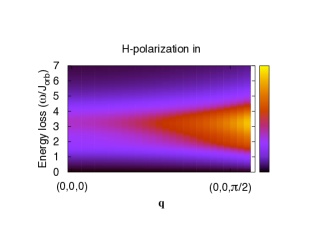
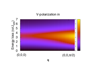
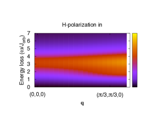
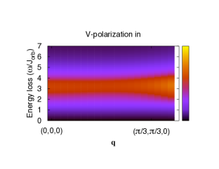
Figure 2: (Color online) RIXS spectra for a model of superexchange-driven orbital order with RIXS coupling to orbitons only via the single site mechanism. The first two spectra are for ${\bf q}$ directed along the $[001]$-direction, the last two for ${\bf q}$ along the $[110]$-direction. The first and third spectrum are for horizontal incoming polarization (electric field in the scattering plane), the second and fourth are for vertical incoming polarization (electric field perpendicular to the scattering plane). Note that the ${\bf q}={\bf 0}$ points are different in each spectrum because of the different experimental geometries, leading to different $P_{\Gamma}$. We only plotted the experimentally accessible part of the Brillouin Zone.

Figure 3: RIXS spectra for a superexchange-driven orbital order with RIXS coupling to orbitons only via the single site mechanism (solid line), compared to the experimental dataexperimentalpaper . The vector ${\bf q}$ is directed along the $[001]$-direction, with $q_{z}$ as indicated in the figures. We took $J_{\rm orb}=80$ meV, and introduced a phenomenological HWHM broadening of $\gamma=0.4\;J_{\rm orb}\approx 30$ meV for the orbitons, as well as the HWHM experimental resolution of $27.5$ meV. The elastic peak is fitted with a Gaussian (dash-dotted line).

Figure 4: Spectra, obtained with the single site mechanism, for the largest experimentally accessible momentum transfer directed along the $[110]$-direction. The solid line indicates the case where the incoming polarization is horizontal, the dashed line is for vertical incoming polarization. The elastic peak has been removed. In the horizontally polarized case, the single orbiton peak is quite strong and should be visible in experiments if the system is superexchange-driven and the RIXS signal is dominated by the single site mechanism.

IV.2 Single site processes – Local model

Although the response functions of the local model of YTiO₃ are entirely different from the superexchange model, the phenomenological scattering operator Eq. (33) is still valid. Focusing on single site processes, Eq. (54) can be evaluated using the wave functions found by Pavarini et al.: Eqs. (5) through (7). Since the eigenstates of the local model have a very simple form, we can straightforwardly use Eqs. (79) through (86) to evaluate the RIXS spectrum. The $P_{\Gamma}$ and $\mathcal{M}_{\Gamma}$ remain the same as in the collective orbiton case. The spectrum now consists of two sharp peaks at $\omega_{1}$ and $\omega_{2}$. These peaks can be broadened by coupling to the lattice as well as due to the superexchange coupling.

Because there are four sublattices which all support their own, local eigenstates, the RIXS intensity can be decomposed into four signals. From the expressions Eqs. (12) through (15), it is easily derived how the $\hat{\Gamma}_{i}$ transform.

So far, the analysis is similar to Sec. IV.1. However, in the local model, the eigenstates are local and this changes the analysis of Sec. IV.1 at two important points. The first one is that the momentum shifts of $\hat{\Gamma}_{\bf q}$ do not destroy interference terms: any final state $\left|f\right>$ can be reached with any shift of ${\bf q}$. All interference terms can in principle be present. The second point to be noted is that, because the eigenstates are local, the only momentum dependence of the cross section comes in through the experimental geometry, which is reflected in the polarization factors $P_{\Gamma}$.

When we compare the theoretical RIXS spectrum of this model to experiment, we again have to take into account the average over the two outgoing polarizations. Assuming again $\mathcal{M}_{\Gamma}$ are the same for all $\Gamma$, and introducing the same broadening as before (HWHM $\gamma\approx 30$ meV phenomenological intrinsic broadening plus $27.5$ meV HWHM experimental broadening), we obtain the spectra shown by the solid lines in Fig. 5.

Figure 5: RIXS spectra for the local model (solid and dashed lines) compared to experimental data experimentalpaper . The vector ${\bf q}$ is directed along the $[001]$-direction, where $q_{z}$ is indicated in the figures. The dashed curve shows the artificially optimized model with degenerate crystal field levels. We introduced a phenomenological intrinsic HWHM broadening ($\gamma\approx 30$ meV [solid line] and $\gamma=100$ meV [dashed line]) for the final states and added experimental broadening.

It is evident that the local model yields a RIXS spectrum that does not agree well with experiment. Firstly, there is no two-peak structure visible in the data. The presence of a two-peak structure in the theoretical curves does not depend on the assumption that all the $\mathcal{M}_{\Gamma}$ are equal. We may finetune the model to produce a better fit by changing the energy levels found in Ref. Pavarini2005, so that both crystal field transitions have an energy of $240$ meV, and introducing a very large intrinsic broadening of $100$ meV (see the dashed lines in Fig. 5). But even in the artificially optimized case of degenerate levels to produce a single peak, the intensity trend remains in contradiction with experiment. Further, it is impossible to tune the energy levels to optimize simultaneously the RIXS and Raman data. Both experiments show a peak at the same energy, while the local model theory predicts the Raman spectra (with its double crystal field excitations) to peak at approximately double the RIXS peak energy.

Even though we could improve the line shape by increasing $\gamma$, the intensity gain with increasing $q_{z}$ cannot be reproduced in any way. In fact, the trend is the opposite: as $q_{z}$ increases, the spectral weight of the theoretical spectrum decreases (see Fig. 5). We recall that the ${\bf q}$-dependence in this case is merely due to polarization factors Eqs. (58$-$67), since in a local picture, each Ti ion contributes independently to the cross section. This is in sharp contrast with the superexchange picture, where the intensity has an intrinsic ${\bf q}$-dependence because of the collective response of all the Ti ions.

Finally, it is hard to reconcile the temperature dependence of the experimental data with the local model. The peak is seen to broaden and lose a large part of its spectral weight with increasing temperatureexperimentalpaper . Ascribing this broadening to phonons has two difficulties. Jahn-Teller active phonons have energies around $30-60$ meV and are therefore not very sensitive to temperature up to $T\approx 350-700$ K. Further, such a broadening would imply a strong orbital-lattice coupling. This then raises the question why no structural phase transition is seen in the titanates. We note that this is very different from, e.g., manganites where orbital-lattice coupling dominates.

IV.3 Two-site processes

The second term in the expansion of the effective scattering operator, Eq. (33), involves two-site processes. Due to the strong multiplet effects, the core hole potential is averaged out and becomes mainly of $A_{1g}$ symmetry. While such a potential cannot directly flip the orbitals at the core hole site, it does affect multi-site processes. In the case of the superexchange model, the core hole potential effectively changes the superexchange constant $J_{SE}$ locally as discussed earlier in the context of RIXS on magnons Brink2007 ; Forte2008A ; Braicovich2009 . This process is illustrated in Fig. 6. (In principle, it is also possible that the core hole potential modifies the orbital interactions via the lattice vibrations.) In this section, we consider the superexchange modulation mechanism to illustrate two-site process in RIXS on orbital fluctuations.

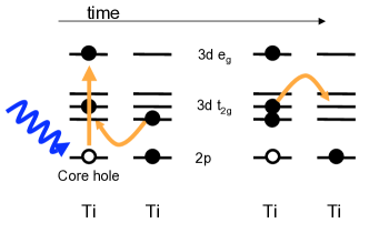
Figure 6: (Color online) In the superexchange model, two-site RIXS processes locally modify the superexchange interaction, coupling the RIXS core hole to the $t_{2g}$ orbitals. Shown is an orbital superexchange process between two neighboring Ti ions in the presence of a core hole. On the left, one of the ions is excited by an incoming x-ray photon. After that, the $t_{2g}$ electrons undergo a superexchange process. On the right, the virtual state of the superexchange process is depicted. The presence of the core hole frustrates the superexchange process. Instead of the usual Hubbard $U$, the energy of the virtual state is lowered by the presence of the positively charged core hole. This modifies the superexchange constant $J_{SE}=4t^{2}/U$ at the core hole site.

The superexchange modification can be derived explicitly by starting from a Hubbard model

$$\tilde{H}= -t\sum_{i}\left(b^{{\dagger}}_{i\pm\hat{x}}b^{\phantom{{\dagger}}}_{i}+c^{{\dagger}}_{i\pm\hat{x}}c^{\phantom{{\dagger}}}_{i}+a^{{\dagger}}_{i\pm\hat{y}}a^{\phantom{{\dagger}}}_{i}+c^{{\dagger}}_{i\pm\hat{y}}c^{\phantom{{\dagger}}}_{i}+a^{{\dagger}}_{i\pm\hat{z}}a^{\phantom{{\dagger}}}_{i}\right.$$

$$\left.+b^{{\dagger}}_{i\pm\hat{z}}b^{\phantom{{\dagger}}}_{i}\right)+U\sum_{i}\left(n_{b,i}n_{c,i}+n_{a,i}n_{c,i}+n_{a,i}n_{b,i}\right)$$

$$-U_{c}\sum_{i}p^{\phantom{{\dagger}}}_{i}p^{{\dagger}}_{i}\left(n_{a,i}+n_{b,i}+n_{c,i}-1\right)$$ (71)

where the last term includes the Coulomb energy $U_{c}$ of the core hole attracting the $t_{2g}$ electrons. $p_{i}$ is the annihilation operator for 2$p$ core electrons at site $i$. We have taken the core hole potential to be of $A_{1g}$ symmetry. Doing perturbation theory to second order in $t/U_{(c)}$ ($U$ and $U_{c}$ are about the same order of magnitude), we obtain the superexchange Hamiltonian

$$H=H_{0}+\sum_{i,\delta}p^{\phantom{{\dagger}}}_{i}p^{{\dagger}}_{i}\left(J_{2}\hat{A}^{(\gamma)}_{i,i+\delta}-J_{1}\hat{n}^{(\gamma)}_{i+\delta}+{\rm const.}\right)$$ (72)

with $\delta$ pointing to nearest neighbors, $n^{(c)}_{i}=n_{a,i}+n_{b,i}$ (the other $n^{(\gamma)}$ can be obtained by permuting the indices $a,b,c$) and

$$J_{1} =\frac{t^{2}}{U-U_{c}}-\frac{t^{2}}{U}$$ (73)

$$J_{2} =\frac{t^{2}}{U+U_{c}}+\frac{t^{2}}{U-U_{c}}-\frac{2t^{2}}{U}$$ (74)

so that $J_{1}/J_{2}=(1+U/U_{c})/2$. Eq. (72) shows we get the unperturbed Hamiltonian plus a contribution which is active only if there is a core hole (in which case $p^{\phantom{{\dagger}}}_{i}p^{{\dagger}}_{i}\rightarrow 1$). The $J_{1}$ term involves single site processes only, and is therefore included in the general description in Sec. IV.1. In the following, the $J_{1}$ term will be dropped.

For simplicity, polarization effects are neglected and we assume $U_{c}$ to be independent of the specific dipole transition. We take

$$\hat{D}=\sum_{i}\left(e^{-i{\bf q}_{\rm in}\cdot{\bf R}_{i}}p^{\phantom{{\dagger}}}_{i}d^{{\dagger}}_{i}+e^{i{\bf q}_{\rm out}\cdot{\bf R}_{i}}p^{{\dagger}}_{i}d^{\phantom{{\dagger}}}_{i}\right)+{\rm h.c.}$$ (75)

with $p_{i}$ the 2$p$ electron annihilation operator and $d_{i}$ the 3$d$ $e_{g}$ electron annihilation operator. The position of the $i^{\rm th}$ site is ${\bf R}_{i}$. The transfered momentum is ${\bf q}={\bf q}_{\rm out}-{\bf q}_{\rm in}$. The neglected polarization dependence could give rise to a ${\bf q}$-dependent factor in the cross section, but will not affect the line shape for a specific ${\bf q}$.

The relevant energy scale for the excitation of orbitons in the intermediate states via superexchange bond modulation is $J_{2}$, as established above, as long as the core hole potential is of $A_{1g}$ symmetry. This is the case when core level spin-orbit coupling and Hund’s rule coupling are large compared to $J_{2}$: the core hole evolves rapidly with time and its potential’s symmetry averages out to $A_{1g}$ before any orbitons can be excited. Because the symmetry is effectively cubic, bonds in all directions are affected in the same way. The effective scattering operator must therefore be a function of $\sum_{\delta}\hat{A}^{(\gamma)}_{i,i+\delta}$ which is of $A_{1g}$ symmetry. Non-linear operators like $\hat{A}^{(\gamma)}_{i,i+\delta}\hat{A}^{(\gamma)}_{i,i+\delta^{\prime}}$ are excluded, they are expected to yield smaller contributions because more and more distant sites are involved. In the expansion Eq. (33), these come in at different orders. The only remaining candidate for the two-site effective scattering operator is therefore

$$\hat{O}_{\bf q}=\mathcal{M}_{2}\sum_{i,\delta}e^{i{\bf q}\cdot{\bf R}_{i}}\hat{A}^{(\gamma)}_{i,i+\delta}$$ (76)

where $\mathcal{M}_{2}$ is an unknown phenomenological matrix element, in the same way as in Sec. IV.1. By construction, the two-site process matrix element $\mathcal{M}_{2}$ should be proportional to $J_{2}$ with a constant determined by the intermediate state dynamical susceptibilities. At this stage, without microscopical calculations of the single-site $\mathcal{M}_{\Gamma}$ (49) and two-site $\mathcal{M}_{2}$ matrix elements, we cannot judge which coupling process dominates the observed RIXS on orbital excitations. Instead, we calculate two-site process independently and compare it with both experimental data and the results obtained above for single-site coupling mechanism.

As it turns out, the two-site effective scattering operator (76) contains only two-orbiton creation terms; it does not create single orbitons because the orbitons are constructed in the first place to diagonalize the Hamiltonian: all linear contributions to $\hat{A}^{(\gamma)}_{ij}$ in Eq. (2) are canceled (similar to the Raman scattering calculations above).

Using again the transformations on the orbital operators mentioned in Ref. [Khaliullin2003, ], condensing the $\psi_{c}$ orbital and transforming to orbiton operators, we obtain for the two-orbiton creation part

$$\hat{O}^{(2)}_{\bf q} =\mathcal{M}_{2}\sum_{\bf k}\left[f_{11}({\bf k},{\bf q})\alpha^{{\dagger}}_{1,{\bf k}}\alpha^{{\dagger}}_{1,-{\bf k}-{\bf q}}\right.$$

$$\left.+f_{22}({\bf k},{\bf q})\alpha^{{\dagger}}_{2,{\bf k}}\alpha^{{\dagger}}_{2,-{\bf k}-{\bf q}}+f_{12}({\bf k},{\bf q})\alpha^{{\dagger}}_{1,{\bf k}}\alpha^{{\dagger}}_{2,-{\bf k}-{\bf q}}\right]$$ (77)

where the $f_{ij}({\bf k},{\bf q})$ are lengthy functions listed in Appendix D. The cross section then is

$$\frac{d^{2}\sigma^{(2)}}{d\omega d\Omega} \propto\sum_{f}\left|\left<f\right|\hat{O}^{(2)}_{\bf q}\left|0\right>\right|^{2}\delta(\omega-\omega_{1/2,{\bf k}}-\omega_{1/2,{\bf k}+{\bf q}})$$

$$=\frac{1}{2}\sum_{\bf k}\left[\left|f_{11}({\bf k},{\bf q})+f_{11}(-{\bf k}-{\bf q},{\bf q})\right|^{2}\times\right.$$

$$\delta(\omega-\omega_{1,{\bf k}}-\omega_{1,{\bf k}+{\bf q}})$$

$$+\left|f_{22}({\bf k},{\bf q})+f_{22}(-{\bf k}-{\bf q},{\bf q})\right|^{2}\times$$

$$\delta(\omega-\omega_{2,{\bf k}}-\omega_{2,{\bf k}+{\bf q}})$$

$$\left.+2\left|f_{12}({\bf k},{\bf q})\right|^{2}\delta(\omega-\omega_{1,{\bf k}}-\omega_{2,{\bf k}+{\bf q}})\right].$$ (78)

The resulting cross section for transfered momenta along the $[001]$ direction is shown in Fig. 7. As in the above sections, we introduced here by hand an energy broadening $\gamma$ of the orbiton states of $\gamma=0.4\;J_{\rm orb}$.

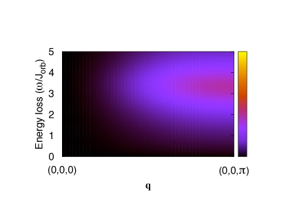
Figure 7: (Color online) RIXS spectrum for two-site processes within the superexchange model. The color scale denotes the intensity. The figure shows ${\bf q}$ running from $(0,0,0)$ to $(0,0,\pi)$. One-orbiton creation is not allowed for the superexchange modulation mechanism. The intrinsic energy broadening $\gamma$ of the orbiton states is $\gamma=0.4\;J_{\rm orb}\approx 30$ meV, and the added experimental resolution of $27.5$ meVexperimentalpaper is approximately $0.34\;J_{\rm orb}$.

A few things should be noted. Firstly, the spectrum disappears at ${\bf q}={\bf 0}$. This is clear from Eq. (76): the scattering operator becomes proportional to the Hamiltonian Eq. (1), giving elastic scattering only.

Secondly, the spectrum shown in Fig. 7 is calculated without taking polarization dependence into account. That could change the relative spectral weight for different ${\bf q}$’s, but does not affect the line shapes.

In Fig. 8 we compare the calculated superexchange spectra for the specific ${\bf q}$ values of the experiments reported in Ref. [experimentalpaper, ]. The only free parameter ($J_{\rm orb}$) gives a best fit for $J_{\rm orb}=75$ meV. As is evident, the increase in spectral weight is qualitatively accounted for by the theory, although the theoretical curves show a much stronger increase with increasing $q_{z}$. We note that one factor that could diminish this discrepancy is, as stated above, the polarization factor we omitted: it could change the relative weight (but not the line shape).

Further, when we compare the theoretical line shapes with the experimental ones, the high energy tail of the experimental data is a bit more intense than in our calculations. This could perhaps be accounted for if one would consider multi-orbiton scattering. Likewise, the shoulder around $\omega=1.5J_{\rm orb}\approx 110$ meV could be due to two-phonon processes. Both these discrepancies depend on the choice of $\gamma$: a larger orbiton damping would transfer spectral weight from the center of the theoretical peak to its tails.

Summarizing, two-site processes can capture some of the features seen in the RIXS data (the intensity trend with increasing momentum transfer, and a single peak without dispersion), but the overall fit is less satisfactory compared to the results of the single-site process shown in Fig. 3.

Figure 8: Theoretical RIXS spectra for two-site processes, calculated within the superexchange model (solid line), compared to experiment experimentalpaper . ${\bf q}$ is directed along the $[001]$-direction, with $q_{z}$ as indicated. We obtain a best fit for $J_{\rm orb}=75$ meV. The solid lines are cuts from the plot of Fig. 7, where we added a Gaussian fit to the elastic peak (dash-dotted line). A phenomenological intrinsic orbiton broadening of $0.4\;r_{1}J_{SE}\approx 30$ meV is added, as well as the experimental resolution of $27.5$ meV (both HWHM)experimentalpaper .

V Conclusions

We have considered two different models, widely discussed in literature to describe orbital physics in titanites, in the context of Raman and x-ray scattering experiments. These models correspond to two limiting cases where the orbital ground state is dominated either by collective superexchange interactions among orbitals or by their coupling to lattice distortions. The models predictions, obtained within the same level of approximations, are compared to the experimental data on Raman (Fig.1) and on x-ray (Figs. 3 and 5) scattering in titanites. What is evident from this comparison and our detailed analysis is that the local crystal field model of YTiO₃ fails to give a coherent explanation of both Raman and RIXS data taken together. There is no way one can get rid of the two-peak structure predicted for RIXS by this model without artificially finetuning its parameters. Further, once tuned to the RIXS spectra, the Raman spectra will be impossible to fit with the local model anyway, since it yields double $dd$-excitations, different from the single crystal field excitations in RIXS. Experimentally, however, both techniques show a peak at the same energy. Also, a huge anisotropy between out-of-plane and in-plane polarizations is predicted by the local model, which is not observed in Raman data. Further, the temperature dependence of the experimental data is hard to explain from a local model: the intensity of crystal field transitions is expected to remain unchanged. Finally, the ${\bf q}$-dependence of the RIXS-intensity is not reproduced by the local model; in fact, the trend is opposite. We believe especially the last four points are robust evidence that the $250$ meV peak seen in Raman and RIXS is not due to local $dd$-excitations.

On the other side, the picture of collective excitations offers much better and broad agreement with the experimental data. The general features of both the Raman and RIXS data are reproduced by the superexchange model. For RIXS we presented a phenomenological scattering operator for single and two-site processes, evaluated within the superexchange model. Although both single and two-site processes the general trends of the RIXS data right, the two-site processes clearly have a too strong ${\bf q}$-dependence of the intensity. The RIXS spectra obtained with the single site operator fit the data very well, suggesting that this process of generating orbitons might be the predominant one in the transition metal oxides. The only slight deviation from the experiments is the one-orbiton peak, which our theory overestimates. However, we note that the theoretical one-orbiton peak is decreased if we consider realistic conditions such as finite temperature and residual spin-orbital quantum fluctuations, which obstruct the orbital order and reduce $\left|c_{0}\right|^{2}$, which in its turn controls the one-orbiton spectral weight.

Ref. [experimentalpaper, ] reported that the RIXS-intensities in LaTiO₃ and YTiO₃ show different ${\bf q}$-dependences: While the intensity in YTiO₃ increases with ${\bf q}$, it decreases in LaTiO₃. On a qualitative level, this contrasting behavior can be understood from the superexchange picture as a manifestation of the (dynamical) Goodenough-Kanamori rules, according to which the spin and orbital correlations are complementary to each other. This implies that the spin and orbital susceptibilities are expected to behave in an opposite fashion. Since magnetic orderings in YTiO₃ and LaTiO₃ are different (ferro- and antiferromagnetic, respectively), collective response of orbitals in these coupounds are expected to be enhanced also at different portions of the Brillouin zone: at large ${\bf q}$ in YTiO₃ and, in contrast, at small ${\bf q}$ in LaTiO₃, which are complementary to the respective locations of their magnetic Bragg peaks. The superexchange picture suggests also that the ${\bf q}$-dependence of the orbiton RIXS-intensity should have cubic symmetry in both LaTiO₃ and YTiO₃, as follows from their isotropic spin-wave Keimer2000 ; Ulrich2002 and Raman spectra Ulrich2006 . Future RIXS experiments in titanites would be useful to verify these expectations.

A previous estimateKhaliullin2003 from neutron spin wave dataUlrich2002 puts the orbital exchange constant $J_{\rm orb}$ at $60$ meV. In close agreement with this estimate, the theoretical Raman spectrum fits best to experiment when $J_{\rm orb}=65$ meV (vertex corrections may change this number, though). Matching to a lesser degree to the estimate, we find for the RIXS spectra $J_{\rm orb}=75$ and $80$ meV for the two-site and single site processes, respectively.

To establish the nature of the $250$ meV peak, it is of great importance to search for the one-orbiton peak. In Raman scattering one-orbiton creation seems to be strongly suppressed, but in RIXS it would be possible to see a one-orbiton peak when ${\bf q}$ is directed maximally along the $[110]$-direction. There the one-orbiton peak (around $\omega\approx 1.8\;J_{\rm orb}\approx 140$ meV) is about as strong as the two-orbiton continuum, assuming single site processes are the dominant RIXS channel, and provided $\left|c_{0}\right|^{2}$ is not too small.

To summarize, we may conclude that the existing Raman and RIXS data in titanites are better described by the superexchange model. This implies that while some polarization of orbitals by static lattice distortions must be a part of a realistic, “ultimate” model for titanites, the orbital fluctuations which are intrinsic to the $t_{2g}$ orbital superexchange process Khaliullin2000 are not yet suppressed and strong enough to stabilize nearly isotropic charge distributions around the Ti-ions.

On the technical side, we believe that our semi-phenomenological approach to the RIXS problem which disentangles the high-energy intermediate state dynamics from low-energy collective excitations of orbitals and spins may serve as a simple and efficient tool in the theoretical description of Resonant Inelastic X-ray Scattering in oxides in general.

VI Acknowledgements

We would like to thank J. van den Brink for stimulating discussions that initiated this work. We also thank B. Keimer, C. Ulrich, and M.W. Haverkort for many fruitful discussions. L.A. thanks the Max-Planck-Institut FKF, Stuttgart, where most of the work was done, for its hospitality.

Appendix A RIXS - Single site processes

The angular momentum $\hat{l}$ and quadrupole operators $\hat{Q},\hat{T}$ in Eqs. (40$-$42) are defined as follows:

$$\hat{l}_{x} =i(c^{{\dagger}}b-b^{{\dagger}}c)$$ (79)

$$\hat{l}_{y} =i(a^{{\dagger}}c-c^{{\dagger}}a)$$ (80)

$$\hat{l}_{z} =i(b^{{\dagger}}a-a^{{\dagger}}b)$$ (81)

$$\hat{Q}_{x} =\hat{l}^{2}_{x}-\hat{l}^{2}_{y}=n_{b}-n_{a}$$ (82)

$$\hat{Q}_{z} =\frac{1}{\sqrt{3}}(\hat{l}^{2}_{x}+\hat{l}^{2}_{y}-2\hat{l}^{2}_{z})=\frac{1}{\sqrt{3}}(2n_{c}-n_{a}-n_{b})$$ (83)

$$\hat{T}_{x} =\hat{l}_{y}\hat{l}_{z}+\hat{l}_{z}\hat{l}_{y}=-(b^{{\dagger}}c+c^{{\dagger}}b)$$ (84)

$$\hat{T}_{y} =\hat{l}_{x}\hat{l}_{z}+\hat{l}_{z}\hat{l}_{x}=-(c^{{\dagger}}a+a^{{\dagger}}c)$$ (85)

$$\hat{T}_{z} =\hat{l}_{x}\hat{l}_{y}+\hat{l}_{y}\hat{l}_{x}=-(a^{{\dagger}}b+b^{{\dagger}}a)$$ (86)

which are normalized by $\text{Tr}\left(\hat{\Gamma}^{2}\right)=2$. The corresponding matrices $\Gamma_{d^{\prime}d}$ in Eq. (38) are

$$\Gamma^{Q_{x}}=\frac{1}{2}\begin{pmatrix}-1&0&0\\ 0&1&0\\ 0&0&0\end{pmatrix},\;\;\; \Gamma^{Q_{z}}=\frac{1}{2\sqrt{3}}\begin{pmatrix}-1&0&0\\ 0&-1&0\\ 0&0&2\end{pmatrix},$$

$$\Gamma^{T_{x}}=-\frac{1}{2}\begin{pmatrix}0&0&0\\ 0&0&1\\ 0&1&0\end{pmatrix},\;\;\; \Gamma^{T_{y}}=-\frac{1}{2}\begin{pmatrix}0&0&1\\ 0&0&0\\ 1&0&0\end{pmatrix},$$

$$\Gamma^{T_{z}}=-\frac{1}{2}\begin{pmatrix}0&1&0\\ 1&0&0\\ 0&0&0\end{pmatrix},\;\;\; \Gamma^{l_{x}}=\frac{1}{2}\begin{pmatrix}0&0&0\\ 0&0&i\\ 0&-i&0\end{pmatrix},$$

$$\Gamma^{l_{y}}=\frac{1}{2}\begin{pmatrix}0&0&-i\\ 0&0&0\\ i&0&0\end{pmatrix},\;\;\; \Gamma^{l_{z}}=\frac{1}{2}\begin{pmatrix}0&i&0\\ -i&0&0\\ 0&0&0\end{pmatrix}$$ (87)

with the indices $d,d^{\prime}=(yz,zx,xy)$ (or for polarization dependence: $\alpha,\beta=(x,y,z)$).

Appendix B Multiplet factors

For the multiplet effect factors in Eq. (43), we have

$$M^{A_{1g}}_{d^{\prime}d} =\sqrt{\frac{2}{3}}\left(\left<d^{\prime}\right|\hat{x}\left|m\right>\left<m\right|\hat{x}\left|d\right>+\left<d^{\prime}\right|\hat{y}\left|m\right>\left<m\right|\hat{y}\left|d\right>\right.$$

$$\left.+\left<d^{\prime}\right|\hat{z}\left|m\right>\left<m\right|\hat{z}\left|d\right>\right)$$ (88)

$$M^{Q_{x}}_{d^{\prime}d} =\left(\left<d^{\prime}\right|\hat{y}\left|m\right>\left<m\right|\hat{y}\left|d\right>-\left<d^{\prime}\right|\hat{x}\left|m\right>\left<m\right|\hat{x}\left|d\right>\right)$$ (89)

$$M^{Q_{z}}_{d^{\prime}d} =\frac{1}{\sqrt{3}}\left(2\left<d^{\prime}\right|\hat{z}\left|m\right>\left<m\right|\hat{z}\left|d\right>-\left<d^{\prime}\right|\hat{x}\left|m\right>\left<m\right|\hat{x}\left|d\right>\right.$$

$$\left.-\left<d^{\prime}\right|\hat{y}\left|m\right>\left<m\right|\hat{y}\left|d\right>\right)$$ (90)

$$M^{T_{x}}_{d^{\prime}d} =-\left(\left<d^{\prime}\right|\hat{y}\left|m\right>\left<m\right|\hat{z}\left|d\right>+\left<d^{\prime}\right|\hat{z}\left|m\right>\left<m\right|\hat{y}\left|d\right>\right)$$ (91)

$$M^{T_{y}}_{d^{\prime}d} =-\left(\left<d^{\prime}\right|\hat{z}\left|m\right>\left<m\right|\hat{x}\left|d\right>+\left<d^{\prime}\right|\hat{x}\left|m\right>\left<m\right|\hat{z}\left|d\right>\right)$$ (92)

$$M^{T_{z}}_{d^{\prime}d} =-\left(\left<d^{\prime}\right|\hat{x}\left|m\right>\left<m\right|\hat{y}\left|d\right>+\left<d^{\prime}\right|\hat{y}\left|m\right>\left<m\right|\hat{x}\left|d\right>\right)$$ (93)

$$M^{l_{x}}_{d^{\prime}d} =-i\left(\left<d^{\prime}\right|\hat{y}\left|m\right>\left<m\right|\hat{z}\left|d\right>-\left<d^{\prime}\right|\hat{z}\left|m\right>\left<m\right|\hat{y}\left|d\right>\right)$$ (94)

$$M^{l_{y}}_{d^{\prime}d} =-i\left(\left<d^{\prime}\right|\hat{z}\left|m\right>\left<m\right|\hat{x}\left|d\right>-\left<d^{\prime}\right|\hat{x}\left|m\right>\left<m\right|\hat{z}\left|d\right>\right)$$ (95)

$$M^{l_{z}}_{d^{\prime}d} =-i\left(\left<d^{\prime}\right|\hat{x}\left|m\right>\left<m\right|\hat{y}\left|d\right>-\left<d^{\prime}\right|\hat{y}\left|m\right>\left<m\right|\hat{x}\left|d\right>\right)$$ (96)

Note that the position operators act on the core electrons, not the $t_{2g}$ ones. Both the core and $t_{2g}$ electrons are implied in the states $\left|d\right>,\left|d^{\prime}\right>$.

Appendix C The operators $\hat{\Gamma}$ in terms of orbitons

In terms of the orbiton operators, we obtain the one-orbiton creation part of $\hat{\Gamma}_{\bf q}=\sum_{i}e^{i{\bf q}\cdot{\bf r}_{i}}\hat{\Gamma}_{i}$ to be

$$\hat{l}^{(1)}_{x,{\bf q}} =\frac{i\left|c_{0}\right|}{2}\sqrt{\frac{N}{3}}\left[\left\{(1-\sqrt{3})u_{{\bf q}_{1}+{\bf q}}+(1+\sqrt{3})v_{{\bf q}_{1}+{\bf q}}\right\}({\rm sh}\;\theta_{1,{\bf q}_{1}+{\bf q}}+{\rm ch}\;\theta_{1,{\bf q}_{1}+{\bf q}})\alpha^{{\dagger}}_{1,-{\bf q}_{1}-{\bf q}}\right.$$

$$+\left.\left\{(-1-\sqrt{3})u_{{\bf q}_{1}+{\bf q}}+(1-\sqrt{3})v_{{\bf q}_{1}+{\bf q}}\right\}({\rm sh}\;\theta_{2,{\bf q}_{1}+{\bf q}}+{\rm ch}\;\theta_{2,{\bf q}_{1}+{\bf q}})\alpha^{{\dagger}}_{2,-{\bf q}_{1}-{\bf q}}\right]$$ (97)

$$\hat{l}^{(1)}_{y,{\bf q}} =\frac{i\left|c_{0}\right|}{2}\sqrt{\frac{N}{3}}\left[\left\{(1+\sqrt{3})u_{{\bf q}_{2}+{\bf q}}+(1-\sqrt{3})v_{{\bf q}_{2}+{\bf q}}\right\}({\rm sh}\;\theta_{1,{\bf q}_{2}+{\bf q}}+{\rm ch}\;\theta_{1,{\bf q}_{2}+{\bf q}})\alpha^{{\dagger}}_{1,-{\bf q}_{2}-{\bf q}}\right.$$

$$+\left.\left\{(-1+\sqrt{3})u_{{\bf q}_{2}+{\bf q}}+(1+\sqrt{3})v_{{\bf q}_{2}+{\bf q}}\right\}({\rm sh}\;\theta_{2,{\bf q}_{2}+{\bf q}}+{\rm ch}\;\theta_{2,{\bf q}_{2}+{\bf q}})\alpha^{{\dagger}}_{2,-{\bf q}_{2}-{\bf q}}\right]$$ (98)

$$\hat{l}^{(1)}_{z,{\bf q}} =-i\left|c_{0}\right|\sqrt{\frac{N}{3}}\left[(u_{{\bf q}_{3}+{\bf q}}+v_{{\bf q}_{3}+{\bf q}})({\rm sh}\;\theta_{1,{\bf q}_{3}+{\bf q}}+{\rm ch}\;\theta_{1,{\bf q}_{3}+{\bf q}})\alpha^{{\dagger}}_{1,-{\bf q}_{3}-{\bf q}}\right.$$

$$+\left.(v_{{\bf q}_{3}+{\bf q}}-u_{{\bf q}_{3}+{\bf q}})({\rm sh}\;\theta_{2,{\bf q}_{3}+{\bf q}}+{\rm ch}\;\theta_{2,{\bf q}_{3}+{\bf q}})\alpha^{{\dagger}}_{2,-{\bf q}_{3}-{\bf q}}\right]$$ (99)

$$\hat{T}^{(1)}_{x,{\bf q}} =\frac{\left|c_{0}\right|}{6}\sqrt{N}\left[\left\{(1+\sqrt{3})u_{{\bf q}_{1}+{\bf q}}+(-1+\sqrt{3})v_{{\bf q}_{1}+{\bf q}}\right\}({\rm ch}\;\theta_{1,{\bf q}_{1}+{\bf q}}-{\rm sh}\;\theta_{1,{\bf q}_{1}+{\bf q}})\alpha^{{\dagger}}_{1,-{\bf q}_{1}-{\bf q}}\right.$$

$$+\left.\left\{(1-\sqrt{3})u_{{\bf q}_{1}+{\bf q}}+(1+\sqrt{3})v_{{\bf q}_{1}+{\bf q}}\right\}({\rm ch}\;\theta_{2,{\bf q}_{1}+{\bf q}}-{\rm sh}\;\theta_{2,{\bf q}_{1}+{\bf q}})\alpha^{{\dagger}}_{2,-{\bf q}_{1}-{\bf q}}\right]$$ (100)

$$\hat{T}^{(1)}_{y,{\bf q}} =\frac{\left|c_{0}\right|}{6}\sqrt{N}\left[\left\{(1-\sqrt{3})u_{{\bf q}_{2}+{\bf q}}+(-1-\sqrt{3})v_{{\bf q}_{2}+{\bf q}}\right\}({\rm ch}\;\theta_{1,{\bf q}_{2}+{\bf q}}-{\rm sh}\;\theta_{1,{\bf q}_{2}+{\bf q}})\alpha^{{\dagger}}_{1,-{\bf q}_{1}-{\bf q}}\right.$$

$$+\left.\left\{(1+\sqrt{3})u_{{\bf q}_{2}+{\bf q}}+(1-\sqrt{3})v_{{\bf q}_{2}+{\bf q}}\right\}({\rm ch}\;\theta_{2,{\bf q}_{2}+{\bf q}}-{\rm sh}\;\theta_{2,{\bf q}_{2}+{\bf q}})\alpha^{{\dagger}}_{2,-{\bf q}_{2}-{\bf q}}\right]$$ (101)

$$\hat{T}^{(1)}_{z,{\bf q}} =-\frac{\left|c_{0}\right|}{3}\sqrt{N}\left[(u_{{\bf q}_{3}+{\bf q}}-v_{{\bf q}_{3}+{\bf q}})({\rm ch}\;\theta_{1,{\bf q}_{3}+{\bf q}}-{\rm sh}\;\theta_{1,{\bf q}_{3}+{\bf q}})\alpha^{{\dagger}}_{1,-{\bf q}_{3}-{\bf q}}\right.$$

$$+\left.(u_{{\bf q}_{3}+{\bf q}}+v_{{\bf q}_{3}+{\bf q}})({\rm ch}\;\theta_{2,{\bf q}_{3}+{\bf q}}-{\rm sh}\;\theta_{2,{\bf q}_{3}+{\bf q}})\alpha^{{\dagger}}_{2,-{\bf q}_{3}-{\bf q}}\right]$$ (102)

$$\hat{Q}^{(1)}_{x,{\bf q}} =\left|c_{0}\right|\sqrt{\frac{N}{3}}\left[-(u_{\bf q}+v_{\bf q})({\rm ch}\;\theta_{1,{\bf q}}-{\rm sh}\;\theta_{1,{\bf q}})\alpha^{{\dagger}}_{1,-{\bf q}}+(u_{\bf q}-v_{\bf q})({\rm ch}\;\theta_{2,{\bf q}}-{\rm sh}\;\theta_{2,{\bf q}})\alpha^{{\dagger}}_{2,-{\bf q}}\right]$$ (103)

$$\hat{Q}^{(1)}_{z,{\bf q}} =-\left|c_{0}\right|\sqrt{\frac{N}{3}}\left[(u_{\bf q}-v_{\bf q})({\rm ch}\;\theta_{1,{\bf q}}-{\rm sh}\;\theta_{1,{\bf q}})\alpha^{{\dagger}}_{1,-{\bf q}}+(u_{\bf q}+v_{\bf q})({\rm ch}\;\theta_{2,{\bf q}}-{\rm sh}\;\theta_{2,{\bf q}})\alpha^{{\dagger}}_{2,-{\bf q}}\right]$$ (104)

with ${\bf q}_{1}=(\pi,0,\pi),\;{\bf q}_{2}=(\pi,\pi,0),\;{\bf q}_{3}=(0,\pi,\pi)$. The expressions for the two-orbiton creation part of $\hat{\Gamma}_{\bf q}=\sum_{i}e^{i{\bf q}\cdot{\bf r}_{i}}\hat{\Gamma}_{i}$ are

$$\hat{l}^{(2)}_{x,{\bf q}} =\frac{i}{\sqrt{3}}\sum_{\bf k}\left[(vu^{\prime}-uv^{\prime}){\rm ch}\;\theta_{1}\;{\rm sh}\;\theta^{\prime}_{1}\;\alpha^{{\dagger}}_{1,{\bf k}}\alpha^{{\dagger}}_{1,-{\bf k}-{\bf q}_{1}-{\bf q}}+(vu^{\prime}-uv^{\prime}){\rm ch}\;\theta_{2}\;{\rm sh}\;\theta^{\prime}_{2}\;\alpha^{{\dagger}}_{2,{\bf k}}\alpha^{{\dagger}}_{2,-{\bf k}-{\bf q}_{1}-{\bf q}}\right.$$

$$+\left.(uu^{\prime}+vv^{\prime})({\rm ch}\;\theta_{1}\;{\rm sh}\;\theta^{\prime}_{2}-{\rm sh}\;\theta_{1}\;{\rm ch}\;\theta^{\prime}_{2})\alpha^{{\dagger}}_{1,{\bf k}}\alpha^{{\dagger}}_{2,-{\bf k}-{\bf q}_{1}-{\bf q}}\right]$$ (105)

with $u,v,\theta_{1},\theta_{2}=u_{\bf k},v_{\bf k},\theta_{1,{\bf k}},\theta_{2,{\bf k}}$ and $u^{\prime},v^{\prime},\theta^{\prime}_{1},\theta^{\prime}_{2}=u_{{\bf k}+{\bf q}_{1}+{\bf q}},v_{{\bf k}+{\bf q}_{1}+{\bf q}},\theta_{1,{\bf k}+{\bf q}_{1}+{\bf q}},\theta_{2,{\bf k}+{\bf q}_{1}+{\bf q}}$. Further, $\hat{l}^{(2)}_{y,{\bf q}}$ and $\hat{l}^{(2)}_{z,{\bf q}}$ have the same form as $\hat{l}^{(2)}_{x,{\bf q}}$ but with ${\bf q}_{1}$ replaced by ${\bf q}_{2}$ and ${\bf q}_{3}$ respectively. Next,

$$\hat{T}^{(2)}_{x,{\bf q}} =\sum_{\bf k}\left[\left\{-(uu^{\prime}+vv^{\prime})+\frac{1}{\sqrt{3}}(uu^{\prime}-vv^{\prime})+\frac{1}{3}(uv^{\prime}+vu^{\prime})\right\}{\rm ch}\;\theta_{1}\;{\rm sh}\;\theta^{\prime}_{1}\;\alpha^{{\dagger}}_{1,{\bf k}}\alpha^{{\dagger}}_{1,-{\bf k}-{\bf q}_{1}-{\bf q}}\right.$$

$$+\left\{-(uu^{\prime}+vv^{\prime})-\frac{1}{\sqrt{3}}(uu^{\prime}-vv^{\prime})-\frac{1}{3}(uv^{\prime}+vu^{\prime})\right\}{\rm ch}\;\theta_{2}\;{\rm sh}\;\theta^{\prime}_{2}\;\alpha^{{\dagger}}_{2,{\bf k}}\alpha^{{\dagger}}_{2,-{\bf k}-{\bf q}_{1}-{\bf q}}$$

$$+\left.\left\{-(uv^{\prime}-vu^{\prime})-\frac{1}{\sqrt{3}}(uv^{\prime}+vu^{\prime})-\frac{1}{3}(uu^{\prime}-vv^{\prime})\right\}({\rm ch}\;\theta_{1}\;{\rm sh}\;\theta^{\prime}_{2}+{\rm sh}\;\theta_{1}\;{\rm ch}\;\theta^{\prime}_{2})\alpha^{{\dagger}}_{1,{\bf k}}\alpha^{{\dagger}}_{2,-{\bf k}-{\bf q}_{1}-{\bf q}}\right]$$ (106)

$$\hat{T}^{(2)}_{y,{\bf q}} =\sum_{\bf k}\left[\left\{-(uu^{\prime}+vv^{\prime})-\frac{1}{\sqrt{3}}(uu^{\prime}-vv^{\prime})+\frac{1}{3}(uv^{\prime}+vu^{\prime})\right\}{\rm ch}\;\theta_{1}\;{\rm sh}\;\theta^{\prime}_{1}\;\alpha^{{\dagger}}_{1,{\bf k}}\alpha^{{\dagger}}_{1,-{\bf k}-{\bf q}_{2}-{\bf q}}\right.$$

$$+\left\{-(uu^{\prime}+vv^{\prime})+\frac{1}{\sqrt{3}}(uu^{\prime}-vv^{\prime})-\frac{1}{3}(uv^{\prime}+vu^{\prime})\right\}{\rm ch}\;\theta_{2}\;{\rm sh}\;\theta^{\prime}_{2}\;\alpha^{{\dagger}}_{2,{\bf k}}\alpha^{{\dagger}}_{2,-{\bf k}-{\bf q}_{2}-{\bf q}}$$

$$+\left.\left\{-(uv^{\prime}-vu^{\prime})+\frac{1}{\sqrt{3}}(uv^{\prime}+vu^{\prime})-\frac{1}{3}(uu^{\prime}-vv^{\prime})\right\}({\rm ch}\;\theta_{1}\;{\rm sh}\;\theta^{\prime}_{2}+{\rm sh}\;\theta_{1}\;{\rm ch}\;\theta^{\prime}_{2})\alpha^{{\dagger}}_{1,{\bf k}}\alpha^{{\dagger}}_{2,-{\bf k}-{\bf q}_{2}-{\bf q}}\right]$$ (107)

where in the expression for $\hat{T}^{(2)}_{y,{\bf q}}$ we replaced ${\bf q}_{1}$ by ${\bf q}_{2}$: $u^{\prime},v^{\prime},\theta^{\prime}_{1},\theta^{\prime}_{2}=u_{{\bf k}+{\bf q}_{2}+{\bf q}},v_{{\bf k}+{\bf q}_{2}+{\bf q}},\theta_{1,{\bf k}+{\bf q}_{2}+{\bf q}},\theta_{2,{\bf k}+{\bf q}_{2}+{\bf q}}$.

$$\hat{T}^{(2)}_{z,{\bf q}} =\sum_{\bf k}\left[\left\{-(uu^{\prime}+vv^{\prime})-\frac{2}{3}(uv^{\prime}+vu^{\prime})\right\}{\rm ch}\;\theta_{1}\;{\rm sh}\;\theta^{\prime}_{1}\;\alpha^{{\dagger}}_{1,{\bf k}}\alpha^{{\dagger}}_{1,-{\bf k}-{\bf q}_{3}-{\bf q}}\right.$$

$$+\left\{-(uu^{\prime}+vv^{\prime})+\frac{2}{3}(uv^{\prime}+vu^{\prime})\right\}{\rm ch}\;\theta_{2}\;{\rm sh}\;\theta^{\prime}_{2}\;\alpha^{{\dagger}}_{2,{\bf k}}\alpha^{{\dagger}}_{2,-{\bf k}-{\bf q}_{3}-{\bf q}}$$

$$+\left.\left\{-(uv^{\prime}-vu^{\prime})+\frac{2}{3}(uu^{\prime}-vv^{\prime})\right\}({\rm ch}\;\theta_{1}\;{\rm sh}\;\theta^{\prime}_{2}+{\rm sh}\;\theta_{1}\;{\rm ch}\;\theta^{\prime}_{2})\alpha^{{\dagger}}_{1,{\bf k}}\alpha^{{\dagger}}_{2,-{\bf k}-{\bf q}_{3}-{\bf q}}\right]$$ (108)

where we replaced ${\bf q}_{1}$ by ${\bf q}_{3}$: $u^{\prime},v^{\prime},\theta^{\prime}_{1},\theta^{\prime}_{2}=u_{{\bf k}+{\bf q}_{3}+{\bf q}},v_{{\bf k}+{\bf q}_{3}+{\bf q}},\theta_{1,{\bf k}+{\bf q}_{3}+{\bf q}},\theta_{2,{\bf k}+{\bf q}_{3}+{\bf q}}$. Finally,

$$\hat{Q}^{(2)}_{x,{\bf q}} =-\frac{1}{\sqrt{3}}\sum_{\bf k}\left[-(uu^{\prime}-vv^{\prime}){\rm ch}\;\theta_{1}\;{\rm sh}\;\theta^{\prime}_{1}\;\alpha^{{\dagger}}_{1,{\bf k}}\alpha^{{\dagger}}_{1,-{\bf k}-{\bf q}}+(uu^{\prime}-vv^{\prime}){\rm ch}\;\theta_{2}\;{\rm sh}\;\theta^{\prime}_{2}\;\alpha^{{\dagger}}_{2,{\bf k}}\alpha^{{\dagger}}_{2,-{\bf k}-{\bf q}}\right.$$

$$+\left.(uv^{\prime}+vu^{\prime})({\rm ch}\;\theta_{1}\;{\rm sh}\;\theta^{\prime}_{2}+{\rm sh}\;\theta_{1}\;{\rm ch}\;\theta^{\prime}_{2})\alpha^{{\dagger}}_{1,{\bf k}}\alpha^{{\dagger}}_{2,-{\bf k}-{\bf q}}\right]$$ (109)

$$\hat{Q}^{(2)}_{z,{\bf q}} =\frac{1}{\sqrt{3}}\sum_{\bf k}\left[(uv^{\prime}+vu^{\prime}){\rm ch}\;\theta_{1}\;{\rm sh}\;\theta^{\prime}_{1}\;\alpha^{{\dagger}}_{1,{\bf k}}\alpha^{{\dagger}}_{1,-{\bf k}-{\bf q}}-(uv^{\prime}+vu^{\prime}){\rm ch}\;\theta_{2}\;{\rm sh}\;\theta^{\prime}_{2}\;\alpha^{{\dagger}}_{2,{\bf k}}\alpha^{{\dagger}}_{2,-{\bf k}-{\bf q}}\right.$$

$$-\left.(uu^{\prime}-vv^{\prime})({\rm ch}\;\theta_{1}\;{\rm sh}\;\theta^{\prime}_{2}+{\rm sh}\;\theta_{1}\;{\rm ch}\;\theta^{\prime}_{2})\alpha^{{\dagger}}_{1,{\bf k}}\alpha^{{\dagger}}_{2,-{\bf k}-{\bf q}}\right]$$ (110)

where in both equations we replaced ${\bf q}_{1}$ by ${\bf 0}$: $u^{\prime},v^{\prime},\theta^{\prime}_{1},\theta^{\prime}_{2}=u_{{\bf k}+{\bf q}},v_{{\bf k}+{\bf q}},\theta_{1,{\bf k}+{\bf q}},\theta_{2,{\bf k}+{\bf q}}$.

Appendix D RIXS - two-site processes with superexchange model

Functions $f_{11},f_{22}$ and $f_{12}$ in Eqs. (77$-$78) are:

$$f_{11}({\bf k},{\bf q}) =\left[-\gamma_{3,{\bf q}}(uv^{\prime}+u^{\prime}v)-\gamma_{2,{\bf q}}(uu^{\prime}-vv^{\prime})-(1+\gamma_{1,{\bf q}})(uu^{\prime}+vv^{\prime})\right]({\rm ch}\;\theta_{1}\;{\rm sh}\;\theta^{\prime}_{1}+{\rm sh}\;\theta_{1}\;{\rm ch}\;\theta^{\prime}_{1})$$

$$+2\left[\gamma^{\prime}_{1}(uu^{\prime}+vv^{\prime})+\gamma^{\prime}_{2}(uu^{\prime}-vv^{\prime})+\gamma^{\prime}_{3}(uv^{\prime}+u^{\prime}v)\right]({\rm sh}\;\theta_{1}\;{\rm sh}\;\theta^{\prime}_{1}+{\rm ch}\;\theta_{1}\;{\rm ch}\;\theta^{\prime}_{1})$$ (111)

$$f_{22}({\bf k},{\bf q}) =\left[\gamma_{3,{\bf q}}(uv^{\prime}+u^{\prime}v)+\gamma_{2,{\bf q}}(uu^{\prime}-vv^{\prime})-(1+\gamma_{1,{\bf q}})(uu^{\prime}+vv^{\prime})\right]({\rm ch}\;\theta_{2}\;{\rm sh}\;\theta^{\prime}_{2}+{\rm sh}\;\theta_{2}\;{\rm ch}\;\theta^{\prime}_{2})$$

$$+2\left[\gamma^{\prime}_{1}(uu^{\prime}+vv^{\prime})-\gamma^{\prime}_{2}(uu^{\prime}-vv^{\prime})-\gamma^{\prime}_{3}(uv^{\prime}+u^{\prime}v)\right]({\rm sh}\;\theta_{2}\;{\rm sh}\;\theta^{\prime}_{2}+{\rm ch}\;\theta_{2}\;{\rm ch}\;\theta^{\prime}_{2})$$ (112)

$$f_{12}({\bf k},{\bf q}) =2\left[\gamma_{3,{\bf q}}(uu^{\prime}-vv^{\prime})+\gamma_{2,{\bf q}}(uv^{\prime}+u^{\prime}v)-(1+\gamma_{1,{\bf q}})(uv^{\prime}-u^{\prime}v)\right]({\rm ch}\;\theta_{1}\;{\rm sh}\;\theta^{\prime}_{2}+{\rm sh}\;\theta_{1}\;{\rm ch}\;\theta^{\prime}_{2})$$

$$+4\left[\gamma^{\prime}_{1}(uv^{\prime}-u^{\prime}v)+\gamma^{\prime}_{2}(uv^{\prime}+u^{\prime}v)-\gamma^{\prime}_{3}(uu^{\prime}-vv^{\prime})\right]({\rm sh}\;\theta_{1}\;{\rm sh}\;\theta^{\prime}_{2}+{\rm ch}\;\theta_{1}\;{\rm ch}\;\theta^{\prime}_{2})$$ (113)

where we shortened notation by writing $\theta_{1/2}=\theta_{1/2,{\bf k}},\;\theta^{\prime}_{1/2}=\theta_{1/2,{\bf k}+{\bf q}},\;u(^{\prime})=u_{{\bf k}(+{\bf q})},\;v(^{\prime})=v_{{\bf k}(+{\bf q})}$ and $\gamma^{\prime}_{i}=\gamma_{i,{\bf k}+{\bf q}}$.

References

• (1) G.A. Gehring and K.A. Gehring, Rep. Prog. Phys. 38, 1 (1975).
• (2) K.I. Kugel and D.I. Khomskii, Sov. Phys. Usp. 25, 231 (1982).
• (3) J.B. Goodenough, Magnetism and Chemical Bond (Interscience Publ., New York-London, 1963.
• (4) G. Khaliullin and S. Okamoto, Phys. Rev. Lett. 89, 167201 (2002).
• (5) G. Khaliullin and S. Okamoto, Phys. Rev. B 68, 205109 (2003).
• (6) B. Keimer, D. Casa, A. Ivanov, J.W. Lynn, M. v. Zimmermann, J.P. Hill, D.Gibbs, Y. Taguchi, and Y. Tokura, Phys. Rev. Lett. 85, 3946 (2000).
• (7) G. Khaliullin and S. Maekawa, Phys. Rev. Lett. 85, 3950 (2000).
• (8) J.-G. Cheng, Y. Sui, J.-S. Zhou, J.B. Goodenough, and W.H. Su, Phys. Rev. Lett. 101, 087205 (2008).
• (9) M. Mochizuki and M. Imada, Phys. Rev. Lett. 91, 167203 (2003).
• (10) E. Pavarini, S. Biermann, A. Poteryaev, A.I. Lichtenstein, A. Georges, and O.K. Andersen, Phys. Rev. Lett. 92, 176403 (2004).
• (11) E. Pavarini, A. Yamasaki, J. Nuss, and O.K. Andersen, New J. Phys. 7, 188 (2005).
• (12) M. Cwik, T. Lorenz, J. Baier, R. Müller, G. André, F. Bourée, F. Lichtenberg, A. Freimuth, R. Schmitz, E. Müller-Hartmann, and M. Braden, Phys. Rev. B 68, 060401(R) (2003).
• (13) R. Schmitz, O. Entin-Wohlman, A. Aharony, A. B. Harris, and E. Müller-Hartmann, Phys. Rev. B 71, 144412 (2005).
• (14) M.W. Haverkort, Z. Hu, A. Tanaka, G. Ghiringhelli, H. Roth, M. Cwik, T. Lorenz, C. Schüßler-Langeheine, S.V. Streltsov, A.S. Mylnikova, V.I. Anisimov, C. de Nadai, N.B. Brookes, H.H. Hsieh, H.-J. Lin, C.T. Chen, T. Mizokawa, Y. Taguchi, Y. Tokura, D.I. Khomskii, and L.H. Tjeng, Phys. Rev. Lett. 94, 056401 (2005).
• (15) I.V. Solovyev, Phys. Rev. B 74, 054412 (2006).
• (16) T. Kiyama and M. Itoh, Phys. Rev. Lett. 91, 167202 (2003).
• (17) M. Kubota, H. Nakao, Y. Murakami, Y. Taguchi, M. Iwama, and Y. Tokura, Phys. Rev. B 70, 245125 (2004).
• (18) T. Kiyama, H. Saitoh, M. Itoh, K. Kodama, H. Ichikawa, and J. Akimitsu, J. Phys. Soc. Jpn. 74, 1123 (2005).
• (19) J. Akimitsu, H. Ichikawa, N. Eguchi, T. Miyano, M. Nishi, and K. Kakurai, J. Phys. Soc. Jpn. 70, 3475 (2001).
• (20) For a review, see G. Khaliullin, Prog. Theor. Phys. Suppl. 160, 155 (2005).
• (21) C. Ulrich, A. Gössling, M. Grüninger, M. Guennou, H. Roth, M. Cwik, T. Lorenz, G. Khaliullin, and B. Keimer, Phys. Rev. Lett. 97, 157401 (2006).
• (22) C. Ulrich, G. Ghiringhelli, A. Piazzalunga, L. Braicovich, N.B. Brookes, H. Roth, T. Lorenz, and B. Keimer, Phys. Rev. B 77, 113102 (2008).
• (23) C. Ulrich, L.J.P. Ament, G. Ghiringhelli, L. Braicovich, M. Moretti Sala, N. Pezzotta, T. Schmitt, G. Khaliullin, J. van den Brink, H. Roth, T. Lorenz, and B. Keimer, Phys. Rev. Lett. 103, 107205 (2009).
• (24) E. Saitoh, S. Okamoto, K.T. Takahashi, K. Tobe, K. Yamamoto, T. Kimura, S. Ishihara, S. Maekawa, and Y. Tokura, Nature 410, 180 (2001).
• (25) M. Grüninger, R. Rückamp, M. Windt, P. Reutler, C. Zobel, T. Lorenz, A. Freimuth, and A. Revcolevschi, Nature 418, 39 (2002).
• (26) E. Saitoh, S. Okamoto, K. Tobe, K. Yamamoto, T. Kimura, S. Ishihara, S. Maekawa, and Y. Tokura, Nature 418, 40 (2002).
• (27) J.P. Goral, J.E. Greedan, and D.A. MacLean, J. Solid State Chem. 43, 244 (1982).
• (28) T. Mizokawa and A. Fujimori, Phys. Rev. B 54, 5368 (1996).
• (29) S. Ishihara, Phys. Rev. B 69, 075118 (2004).
• (30) P. Knoll, C. Thomsen, M. Cardona, and P. Murugaraj, Phys. Rev. B 42, 4842(R) (1990).
• (31) R. Rückamp, E. Benckiser, M.W. Haverkort, H. Roth, T. Lorenz, A. Freimuth, L. Jongen, A. Möller, G. Meyer, P. Reutler, B. Büchner, A. Revcolevschi, S.-W. Cheong, C. Sekar, G. Krabbes, and M. Grüninger, New J. Phys. 7, 144 (2005).
• (32) P.A. Fleury and R. Loudon, Phys. Rev. 166, 514 (1968).
• (33) R.J. Elliott and R. Loudon, Phys. Lett. 3, 189 (1963).
• (34) S. Miyasaka, S. Onoda, Y. Okimoto, J. Fujioka, M. Iwama, N. Nagaosa, and Y. Tokura, Phys. Rev. Lett. 94, 076405 (2005).
• (35) C. Ulrich, G. Khaliullin, S. Okamoto, M. Reehuis, A. Ivanov, H. He, Y. Taguchi, Y. Tokura, and B. Keimer, Phys. Rev. Lett. 89, 167202 (2002).
• (36) J. van den Brink, Europhys. Lett. 80, 47003 (2007).
• (37) J.P. Hill, G. Blumberg, Y.-J. Kim, D.S. Ellis, S. Wakimoto, R.J. Birgeneau, S. Komiya, Y. Ando, B. Liang, R.L. Greene, D. Casa, and T. Gog, Phys. Rev. Lett. 100, 097001 (2008).
• (38) F. Forte, L.J.P. Ament, and J. van den Brink, Phys. Rev. B 77, 134428 (2008).
• (39) F. Forte, L.J.P. Ament, and J. van den Brink, Phys. Rev. Lett. 101, 106406 (2008).
• (40) L. Braicovich, L.J.P. Ament, V. Bisogni, F. Forte, C. Aruta, G. Balestrino, N.B. Brookes, G.M. De Luca, P.G. Medaglia, F. Miletto Granozio, M. Radovic, M. Salluzzo, J. van den Brink, and G. Ghiringhelli, Phys. Rev. Lett. 102, 167401 (2009).
• (41) J. van den Brink and M. van Veenendaal, J. Phys. Chem. Solids 66, 2145 (2005).
• (42) L.J.P. Ament, F. Forte, and J. van den Brink, Phys. Rev. B 75, 115118 (2007).
• (43) J.D. Garrett, J.E. Greedan, and D.A. MacLean, Mater. Res. Bull. 16, 145 (1981).