Phase transition in the two-dimensional dipolar Planar Rotator model

Abstract

In this work we have used extensive Monte Carlo simulations and finite size scaling theory to study the phase transition in the dipolar Planar Rotator model (dPRM) , also known as dipolar XY model. The true long-range character of the dipolar interactions were taken into account by using the Ewald summation technique. Our results for the critical exponents does not fit those from known universality classes. We observed that the specific heat is apparently non-divergent and the critical exponents are $\nu=1.277(2)$, $\beta=0.2065(4)$ and $\gamma=2.218(5)$. The critical temperature was found to be $T_{c}=1.201(1)$. Our results are clearly distinct from those of a recent Renormalization Group study from Maier and Schwabl [PRB 70, 134430 (2004)] and agrees with the results from a previous study of the anisotropic Heisenberg model with dipolar interactions in a bilayer system using a cut-off in the dipolar interactions [PRB 79, 054404 (2009)].

I Introduction

The Planar Rotator model (PRM) in two dimensions, also known as XY model, is known to have a critical line in the low temperature region Wegner (1967); Berezinskii (1971); Kosterlitz and Thouless (1973). The PRM is described by the following Hamiltonian: $H=-J\sum_{<i,j>}\vec{S}_{i}\cdot\vec{S}_{j}=-J\sum_{<i,j>}(S^{x}_{i}S^{x}_{j}+S^{y}_{i}S^{y}_{j})$, where $\vec{S}_{i}$ is a two dimensional vector $(S^{x}_{i},S^{y}_{i})$ defined in the sites $i$ of a two-dimensional lattice and $<i,j>$ means that the summation is to be evaluated for nearest neighbors sites. As a prototype the PRM is expected to describe the magnetic properties of ferromagnetic thin films where the spins lie in the film plane. Although very simple, this model presents some unusual characteristics, as the absence of spontaneous magnetization for any $T>0$, which is a consequence of the Mermin and Wagner theorem Mermin and Wagner (1966). Thus, the system can not have a phase transition of order-disorder type, nevertheless, there is still a phase transition in the model characterized by a change in the spin-spin correlation function behavior. It is observed an algebraic decay of the correlation function below a characteristic temperature, $T_{BKT}$, above which the decaying is exponential. Besides that, the correlation length is expected to diverge exponentially as long as $T_{BKT}$ is approached from above, i.e., $\xi(r)\sim a\exp{(b/\sqrt{T-T_{BKT}})}$ for $T>T_{BKT}$, while it remains infinity for any $T<T_{BKT}$. This transition is named Berezinskii-Kosterlitz-Thouless ($BKT$) phase transition Berezinskii (1971); Kosterlitz and Thouless (1973). Several works, analytical as well as numerical, dealing with the subject were published since the seminal work of Berezinskii and Kosterlitz and Thouless Minnhagen (1987); Hikami and Tsuneto (1980); Takeno and Homma (1980); Evertz and Landau (1996); Costa and Costa (1996). Besides that, it is also observed that the specific heat does not diverge, instead, it has a broad maximum at a temperature slightly higher than $T_{BKT}$ Cuccoli et al. (1995); Gupta and Baillie (1992); Olson (1973); Lima and Costa (2003). There are two interpretations for the mechanism leading to this transition: Berezinskii Berezinskii (1971) and Kosterlitz and Thouless Kosterlitz and Thouless (1973) assume that it is driven by a vortex-anti-vortex unbinding mechanism, while Patrascioiu and Seiler Patrascioiu and Seiler (1988) were able to obtain the critical temperature and predicted the existence of a phase transition in the Coulomb gas in any dimension ($d>1$) by considering that the mechanism responsible for the transition is a polymerization of domain walls. (As a matter of unification of language we use in this paper the terminology $BKT$ for this kind of transition).

However, in order to achieve a deeper insight on the magnetic properties of thin films, one has to include dipolar interactions between the magnetic moments of the lattice. This inclusion changes the scenario drastically, as discussed by Maleev Maleev (1976). The long-range dipolar interactions stabilizes the magnetization at low temperatures in such a way that an order-disorder phase transition is now expected to take place. In a recent paper, Maier and Schwabl Maier and Schwabl (2004) have analyzed the phase transition in the dipolar Planar Rotator model (dPRM) by using renormalization group techniques. Their results indicate that the dPRM belongs to a new universality class characterized by an exponential behavior of the magnetization, susceptibility and correlation length. Besides that, the specific heat was found to be non-divergent, like occurs in the $BKT$ phase transition. In this work, we have used extensive Monte Carlo simulations to study the phase transition in the dPRM. Our results clearly indicate that the transition is of order-disorder type and is characterized by a non-divergent specific heat and unusual critical exponents.

II dipolar Planar Rotator model and Monte Carlo method

The model we are interested in consists of a square lattice with dimension $L\times L$. At each site we place a classical spin variable $\vec{S}_{i}=(S^{x}_{i},S^{y}_{i})$ with $\vec{S}_{i}^{2}=1$. The interactions are defined by the following Hamiltonian:

$$H=-J\sum_{<i,j>}\vec{S}_{i}\cdot\vec{S}_{j}+D\sum_{i\neq j}\left[\frac{\vec{S}_{i}\cdot\vec{S}_{j}}{r_{ij}^{3}}-\frac{3(\vec{S}_{i}\cdot\vec{r}_{ij})(\vec{S}_{j}\cdot\vec{r}_{ij})}{r_{ij}^{5}}\right].$$ (1)

Here, $J>0$ defines a ferromagnetic exchange constant and $D$ is the dipolar constant. $\vec{r}_{ij}$ connects sites $i$ and $j$ while $<i,j>$ means that the first summation is evaluated for nearest neighbors only. For the dipolar interactions the summation is evaluated over all pairs $i\neq j$. Periodic boundary conditions have been used in the film plane ($x$ and $y$ directions) while open boundary conditions were applied in the $z$ direction. Ewald summation techniques Weis (2003); Wang and Holm (2001) have been used to take into account the true long-range character of the dipolar interactions. In all simulations we have assumed $J=1$ and $D=0.1$ and for these values only ferromagnetic configurations were found in the low temperature regime. In this work the energy is measured in units of $JS^{2}$ and temperature in units of $JS^{2}/k_{B}$.

Our Monte Carlo procedure consists of a simple Metropolis algorithm Metropolis et al. (1953); Landau and Binder (2005) where one Monte Carlo step (MCS) consists of an attempt to assign a new random direction to each spin in the lattice. To equilibrate the system we have used $100\times L^{2}$ MCS which has been found to be sufficient to reach equilibrium, even in the vicinity of the transition. In our scheme, two sets of simulations have been performed. In the first one, we preliminarily explored the thermodynamic behavior of the model in order to estimate the position of the maxima of the specific heat and susceptibilities and the crossings of the fourth order Binder’s cumulant. In this first approach we used lattice sizes in the interval $20\leq L\leq 50$. Once the possible transition temperature is determined, we refined the results by using single and multiple histogram methods Ferrenberg (1991); Ferrenberg and Swendsen (1989). We produced the histograms for each lattice size in the interval $20\leq L\leq 120$ and they were built at/close to the estimated critical temperatures corresponding to the maxima and/or crossing points obtained in step 1. Details of the histogram techniques can be found in Refs. Ferrenberg (1991); Ferrenberg and Swendsen (1989).

III Thermodynamic quantities and finite size scaling theory

We have devoted our efforts to determine a number of thermodynamical quantities, namely, the specific heat, magnetization, susceptibility, fourth order Binder’s cumulant and moments of magnetization as described below. The specific heat is defined as:

$$c_{v}=\frac{\langle E^{2}\rangle-\langle E\rangle^{2}}{Nk_{B}T^{2}},$$ (2)

where $E$ is the internal energy of the system (computed using equation 1) and $N=L^{2}$ is the lattice volume. The magnetization is:

$$M=\frac{1}{N}\langle m\rangle$$ (3)

where

$$m=\sqrt{\left(\sum_{i=1}^{N}S^{x}_{i}\right)^{2}+\left(\sum_{i=1}^{N}S^{y}_{i}\right)^{2}}.$$ (4)

The susceptibility is defined by the magnetization fluctuations as:

$$\chi_{xy}=\frac{\langle m^{2}\rangle-\langle m\rangle^{2}}{Nk_{B}T}.$$ (5)

The fourth order Binder’s cumulant reads:

$$U_{4}=1-\frac{\langle m^{4}\rangle}{3\langle m^{2}\rangle^{2}}.$$ (6)

In order to calculate the critical exponent $\nu$, we also define the following moments of the magnetization Chen et al. (1993):

$$V_{1} \equiv 4[m^{3}]-3[m^{4}],$$ (7a)

$$V_{2} \equiv 2[m^{2}]-[m^{4}],$$ (7b)

$$V_{3} \equiv 3[m^{2}]-2[m^{3}],$$ (7c)

$$V_{4} \equiv (4[m]-[m^{4}])/3,$$ (7d)

$$V_{5} \equiv (3[m]-[m^{3}])/2,$$ (7e)

$$V_{6} \equiv 2[m]-[m^{2}],$$ (7f)

where,

$$[m^{n}]\equiv\ln\left|\frac{\partial\langle m^{n}\rangle}{\partial T}\right|.$$ (8)

In critical phenomena the thermodynamic quantities are expect to behave in the vicinity of the phase transition as Stanley (1971); Privman (1990); Landau and Binder (2005):

$$c_{v}\sim t^{-\alpha}$$ (9a)

$$\chi\sim t^{-\gamma}$$ (9b)

$$M\sim t^{\beta}$$ (9c)

$$\xi\sim t^{-\nu},$$ (9d)

where $t=|T-T_{c}|/T_{c}$ is the reduced temperature, $M$ is the magnetization, $\xi$ is the correlation length and $\alpha$, $\beta$, $\gamma$ and $\nu$ are critical exponents. Although the critical temperature depends on the details of the system in consideration, it is observed that the critical exponents are universal, depending only on a few fundamental factors Stanley (1971); Privman (1990); Landau and Binder (2005). The systems are thus divided in a small number of universality classes. Systems belonging to the same universality class share the same critical exponents. Critical exponents are observed to depend only on the spatial dimensionality of the system, the symmetry and dimensionality of the order parameter, and the range of the interactions within the system.

In a finite system as those used in Monte Carlo simulations the divergences in the thermodynamic quantities are replaced by smooth functions. Finite size effects are therefore of great importance in the analysis of the results of Monte Carlo simulations. The theory of finite size scaling Privman (1990); Landau and Binder (2005) provides one way to extract information concerning the thermodynamic limit properties from results obtained in finite systems. The basic assumption of this theory is that in the vicinity of the phase transition the finite size effects should depend on the ratio between the linear dimension of the system and the correlation length say, $L/\xi$ . According to such a theory, specific heat, susceptibility and magnetization for a finite system, in the vicinity of the phase transition, behave as:

$$c_{v}\approx c_{\infty}(t)+L^{\alpha/\nu}\mathbf{\mathcal{C}}(tL^{1/\nu}),$$ (10a)

$$\chi\approx L^{\gamma/\nu}\mathbf{\mathcal{X}}(tL^{1/\nu}),$$ (10b)

$$M\approx L^{-\beta/\nu}\mathbf{\mathcal{M}}(tL^{1/\nu}),$$ (10c)

where $\mathbf{\mathcal{M}}$, $\mathbf{\mathcal{X}}$ and $\mathbf{\mathcal{C}}$ are proper derivatives of the free energy. At $T_{c}$ ($t=0$) these functions are constants and the size dependence of specific heat, susceptibility and magnetization follow a pure power law. The size dependence of the pseudo-critical temperature, $T_{c}(L)$, is Privman (1990); Landau and Binder (2005)

$$T_{c}(L)=T_{c}+wL^{-1/\nu},$$ (11)

where $T_{c}$ is the critical temperature in the thermodynamic limit. Using the size dependence of the magnetization, equation 10, and the definition of the moments of the magnetization in equation 7, one can easily show that such functions behave as:

$$V_{j}\approx(1/\nu)\ln L+\mathcal{V}_{j}(tL^{1/\nu}),$$ (12)

for $j=1,2,...,6$. At $t=0$ the functions $\mathcal{V}_{j}(tL^{1/\nu})$ are constants and then the curves for all $V_{j}$ have the same slope Chen et al. (1993) providing a very precise method to determine both the critical exponent $\nu$ and the critical temperature.

Concerning the fourth order Binder’s cumulant, it is expected that its curves should cross at the same point $U^{*}=U(T=T_{c})$ for large enough $L$. Besides that, its size dependence is expected to obeys Binder (1981):

$$U_{4}\approx\mathcal{U}_{4}(tL^{1/\nu}).$$ (13)

IV Results

In the following we show the results obtained by using the histogram method. Each histogram consists of at least $3\times 10^{7}$ configurations. In figure 1 we show a log-log plot of the maxima of the susceptibility as a function of the lattice size for $L=20,40,80$ and $120$. The data are very well adjusted by a straight line with slope $\gamma/\nu=1.737(1)$ exhibiting a power law behavior. The specific heat maxima as a function of the lattice size are shown in figure 2. In this figure, the solid line represents the best non-linear adjust of a logarithmic divergence while the dashed one the best power law divergence adjust. It is clear that none of then can adjust our data satisfactorily. This result is similar to that obtained for the PRM without dipolar interactions, and indicates a possible non-divergent specific heat. In figure 3 we show the value of $1/\nu$ for some temperatures obtained by using the moments of the magnetization defined in equation 7 and 12. Using this method we get $T_{c}^{V_{j}}=1.1982(18)$ and $1/\nu=0.74(2)$.

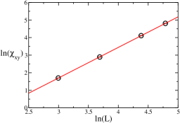
Figure 1: Log-log plot of the maxima of susceptibility as a function of the lattice size for $L=20,40,80$ and $120$. The error bars are shown inside the symbols. The straight line is the best linear fit which gives the exponent $\gamma/\nu=1.737(1)$.

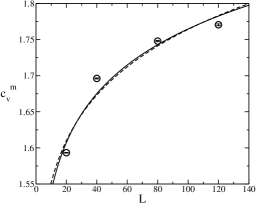
Figure 2: Specific heat maxima as a function of the lattice size. The solid line is the best non-linear fit considering a logarithmic divergence and the dashed line is the best fit considering a power law divergence. The error bars are shown inside the symbols.

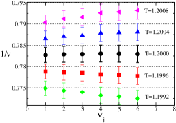
Figure 3: Value of $1/\nu$ obtained by linear fits of $V_{j}$ versus $\ln(L)$ for each value of $j$ at different temperatures. Note that for $T=1.2000$ the value of $1/\nu$ is almost the same for all quantities.

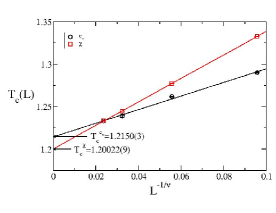
Figure 4: $T_{c}(L)$ versus $L^{-1/\nu}$. From a linear adjust we get $T_{c}^{\chi}=1.20022(9)$ and $T_{c}^{c_{v}}=1.2150(3)$.

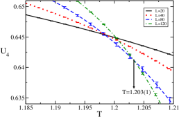
Figure 5: Fourth order Binder’s cumulant. The critical temperature was estimated by the crossing point of the largest lattice sizes as being $T_{c}^{U_{4}}=1.203(1)$. Only a few error bars are shown for clarity.

With the value of $1/\nu$ we may estimate the critical temperature using the finite size scaling properties of the maxima of the susceptibility and specific heat, see equation 11. In figure 4 we show a plot of $T_{c}(L)$ as a function of $L^{-1/\nu}$. We obtain $T_{c}^{\chi}=1.20022(9)$ and $T_{c}^{c_{v}}=1.2150(3)$. Using the crossing points of the fourth order Binder’s cumulant Binder (1981), see figure 5, we estimate the critical temperature $T_{c}^{U_{4}}=1.203(1)$. Our best value for the critical temperature is thus the mean value of the previous estimates $T_{c}^{U_{4}}$, $T_{c}^{V_{j}}$ and $T_{c}^{\chi}$ discarding the value obtained by finite size scaling of the specific heat, since its behavior is apparently non-critical. This procedure gives $T_{c}=1.201(1)$. Plotting $\ln(M_{xy})$ versus $\ln(L)$ at $T_{c}$ it is possible to obtain the exponent $\beta/\nu$. From a linear adjust we get $\beta/\nu=0.1617(2)$. In order to verify the validity of our results we show in figures 6, (7) and (8), the scaling plots of the susceptibility, magnetization and fourth order Binder’s cumulant according to their finite size scaling functions, see equation 10. Note that all figures show a very good collapse of the curves for different lattice sizes.

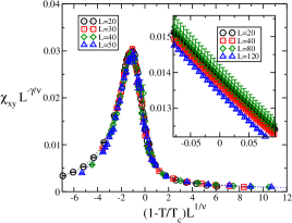
Figure 6: Scaling plot of susceptibility. According to finite size scaling theory Privman (1990); Landau and Binder (2005) the susceptibility is expected to behave as $\chi\approx L^{\gamma/\nu}\mathbf{\mathcal{X}}(tL^{1/\nu})$. Note that the curves for different lattice sizes collapses into a single curve. In the outer plot the scaling is done using results from conventional Monte Carlo simulations (step 1) for $L=20,30,40$ and $50$. The inset shows the scaling for the histogram results (step $2$ in our simulations) for $L=20,40,80,120$.

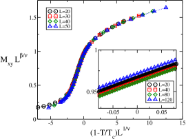
Figure 7: Scaling plot of magnetization. According to finite size scaling theory Privman (1990); Landau and Binder (2005) this quantity is expected to behave as $m\approx L^{-\beta/\nu}\mathbf{\mathcal{M}}(tL^{1/\nu})$. Note that the curves for different lattice sizes collapses into a single curve. In the outer plot the scaling is done using results from conventional Monte Carlo simulations (step 1) for $L=20,30,40$ and $50$. The inset shows the scaling for the histogram results (step $2$ in our simulations) for $L=20,40,80,120$.

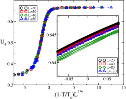
Figure 8: Scaling plot of the fourth order Binder’s cumulant. According to finite size scaling theory Binder (1981) this quantity is expected to behave as $U_{4}\approx\mathcal{U}_{4}(tL^{1/\nu})$. Note that the curves for different lattice sizes collapses into a single curve. In the outer plot the scaling is done using results from conventional Monte Carlo simulations (step 1) for $L=20,30,40$ and $50$. The inset shows the scaling for the histogram results (step $2$ in our simulations) for $L=20,40,80,120$.

V Discussion

In this work we have studied the phase transition in the ferromagnetic dipolar Planar Rotator model (dPRM). Our results indicate that the phase transition in this model is of order-disorder type and is characterized by the exponents $\nu=1.277(2)$, $\beta=0.2065(4)$ and $\gamma=2.218(5)$ and by a non-divergent specific heat. Our results also indicate that the system have long-range order at low temperatures. This conclusion is based on the following facts: ($i$) the magnetization for $T<T_{c}$ does not display a significant decrease as the lattice size is augmented, as for example, has been found in the Rapini’s work Rapini et al. (2007) and as expected for a BKT phase transition; ($ii$) our results are very well described by a finite size scaling theory based on the existence of a low temperature phase with long-range order and finite correlation length Privman (1990); Landau and Binder (2005). In a BKT phase transition there is no long-range order in the low temperature phase as a consequence of the Mermin-Wagner theorem Mermin and Wagner (1966). Indeed, the results of Maleev Maleev (1976) predict the existence of long-range order at low temperatures in the dPRM and our results are consistent with this scenario.

As discussed earlier, recent results by Maier and Schwabl Maier and Schwabl (2004) have predicted that this system may belong to a new universality class, characterized by the presence of long-range order at low temperatures and by an exponential behavior of thermodynamic quantities in the vicinity of the “critical” temperature. By an exponential divergence we mean that the correlation length diverges as the “critical” temperature ($T_{c}$) is approached as $\xi\propto\exp(b/\sqrt{(T-T_{c})})$, similarly to the behavior of the BKT phase transition, while the behavior of other thermodynamic quantities are given by powers of the correlation length. Nevertheless, our results for the dPRM are very well described by power law divergences of thermodynamic quantities. As can be seen in figures 6, 7 and 8, we obtained a very good collapse of the curves from different lattice sizes for the susceptibility, magnetization and Binder’s cumulant. These curves show that the critical exponents obtained and the conventional finite size scaling theory, that assumes a power law behavior of thermodynamic quantities, describe the Monte Carlo data accurately indicating that the phase transition in the dPRM is a conventional order-disorder phenomena with unusual critical exponents. In order to definitely rule out the possibility of this phase transition of being in the new universality class proposed by Maier and Schwabl, we should make a comparison of our Monte Carlo results, using a finite size scaling theory based in their predictions, and the conventional finite size scaling theory used here. Unfortunately, it is not clear in the literature how to obtain a finite size scaling theory for exponential divergences. Using a simple replacement of the correlation length by the lattice size, which should be the first choice, does not give a good collapse of the curves, mainly because the determination of the critical temperature is quite imprecise in this case and the collapse of the curves depend appreciably on the value used for the critical temperature. In any case, using values for the critical temperature close to the maxima of the susceptibility we were not able to obtain even a reasonable collapse of the curves.

Once the possibility of this phase transition being in the new universality class proposed by Maier and Schwabl is discarded, some questions arise: ($i$) Why Renormalization Group results do not agree with our Monte Carlo simulations? ($ii$) Is the occurrence of the order-disorder transition due to the long-range character of dipolar interactions or to some other property of this model? A definite answer to these questions may take a very long time to be given by virtue of the non-trivial characteristics presented by this model. Nevertheless, this study gave us some insight about what is happening. The RG study of Maier and Schwabl Maier and Schwabl (2004) is based upon some approximations, for instance, the using of a continuous version of dPRM, where the lattice character is lost. Since the dipolar interactions have an intrinsic anisotropy which depends in a complicated manner on the location of each spin in the lattice, the lattice geometry could have an strong effect in the system. The identification and discussion of the finer points of the RG study of the dPRM that cause the discrepancy in the results is beyond the scope of this paper. Concerning the origin of the order-disorder transition the question is even more complicated. The long-range order observed at low temperatures is expected to occur only when full long-range interactions are present. Nevertheless, in a recent study of the anisotropic Heisenberg model in a bilayer system Mól and Costa (2009) using a cut-off in the dipolar interactions we found the same critical behavior. In fact, the found critical exponents ($\nu=1.22(9)$, $\gamma=2.1(2)$ and $\beta=0.18(5)$) agree inside the errors with those found in this study ($\nu=1.277(2)$, $\beta=0.2065(4)$ and $\gamma=2.218(5)$). This observation indicates that the anisotropic character of dipolar interactions may be the main responsible by the observed critical phenomena. Indeed, this observation is not new in the literature. As an example, Fernández and Alonso Fernández and Alonso (2007) stated that “Anisotropy has a deeper effect on the ordering of systems of classical dipoles in 2D than the range of dipolar interactions”. In this work the authors found that the inclusion of a quadrupolar anisotropy changes drastically the phase transition behavior of a system of classical dipoles. Apparently, in our system the intrinsic anisotropy of dipolar interactions play an essential role in the determination of the universality class of the dPRM.

The possible new universality class is not surprising. In the theory of critical phenomena Privman (1990); Landau and Binder (2005) it is expected that the critical exponents, and thus the universality classes, depend only on the spatial dimensionality of the system, the symmetry and dimensionality of the order parameter, and the range of the interactions within the system, characteristics not shared by the dPRM and models of well known universality classes. To the best of our knowledge this work and that of Maier and Schwabl Maier and Schwabl (2004) are the only ones devoted to the investigation of the critical behavior of systems with long-range dipolar interactions (which are intrinsically anisotropic) and exchange interactions in two dimensions.