Combinatorial descriptions of
multi-vertex $2$-complexes

Abstract.

Group presentations are implicit descriptions of $2$-dimensional cell complexes with only one vertex. While such complexes are usually sufficient for topological investigations of groups, multi-vertex complexes are often preferable when the focus shifts to geometric considerations. In this article, I show how to quickly describe the most important multi-vertex $2$-complexes using a slight variation of the traditional group presentation. As an illustration I describe multi-vertex $2$-complexes for torus knot groups and one-relator Artin groups from which their elementary properties are easily derived. The latter are used to give an easy geometric proof of a classic result of Appel and Schupp.

Some cell complexes are easy to describe: a graph with one vertex corresponds to a set $S$ indexing its edges and a one-vertex combinatorial $2$-complex can be constructed from an algebraic presentation $\langle S\mid\mathcal{R}\rangle$. When one tries to describe $2$-complexes with multiple vertices, however, several issues arise. First, there is no standard way to quickly describe a complicated $1$-complex. And second, even supposing such a $1$-skeleton as given with edges oriented and labeled by a set $S$, not all words over the alphabet $S\cup S^{-1}$ can be used to describe closed paths, making it easy to list collections of words that are incompatible with the given graph. In this article we describe a simple procedure that avoids both of these difficulties and requires only mild restrictions. It constructs a multi-vertex link-connected combinatorial $2$-complex from any multiset of words, and every such complex can be constructed in this way. Such a process is sufficient for most purposes since the only $2$-complexes excluded are those that are homotopy equivalent to a non-trivial wedge product, i.e. those whose fundamental groups can be freely decomposed. After describing this procedure and establishing its main properties, sample applications are given that illustrate how multi-vertex complexes can make geometric properties of groups more transparent, including a short geometric proof of a classic result of Appel and Schupp [2].

1. Standard $2$-complexes

We begin by reviewing the standard method for creating a one-vertex combinatorial $2$-complex from an algebraic presentation $\langle S\mid\mathcal{R}\rangle$. Recall that CW complexes are inductively constructed by attaching $n$-discs along their boundary cycles to an already constructed $(n-1)$-skeleton and that $1$-dimensional CW complexes are undirected graphs. Recall also that a map $Y\rightarrow X$ between CW complexes is a combinatorial map if its restriction to each open cell of $Y$ is a homeomorphism onto an open cell of $X$ and that a CW complex $X$ is combinatorial provided that the attaching map of each cell of $X$ is combinatorial for a suitable subdivision of its domain. In this article all maps and cell complexes are combinatorial unless otherwise specified. For a $2$-complex, this means that it can be viewed as the result of attahing polygons to a graph using combinatorial maps.

Definition 1.1 (Polygons and $2$-complexes).

A polygon is a (closed) $2$-disc $\mathbb{D}^{2}$ whose boundary cycle has been given the structure of a graph. When its boundary cycle has combinatorial length $n$ it is called an $n$-gon. A $2$-complex $X$ is constructed from a graph $\Gamma$ and a collection $\mathcal{P}$ of disjoint polygons by specifying for each $n$-gon in $\mathcal{P}$ a closed combinatorial path of length $n$ in $\Gamma$ along which its boundary cycle should be attached. Let $P$ denote the disjoint union of polygons in $\mathcal{P}$ and note that $P$ itself is a cell complex. Also note that so long as $X$ has no isolated vertices and every edge of $\Gamma$ occurs in the image of at least one attaching map, the complex $X$ is a quotient of the complex $P$ and the quotient map $P\twoheadrightarrow X$ is a combinatorial map. When $X$ satisfies these minor restrictons, we say that $X$ is a polygon quotient with quotient map $P\twoheadrightarrow X$.

A $2$-complex with only one vertex is called a standard $2$-complex and the traditional way to quickly and efficiently describe it is via a presentation.

Definition 1.2 (Presentations).

A presentation $\langle S\mid\mathcal{R}\rangle$ consists of a set $S$ and a multiset of words $\mathcal{R}$ over the alphabet $S\cup S^{-1}$. (We say multiset rather than set because repetitions are allowed.) The elements of $S$ are generators and the elements of $\mathcal{R}$ are relators.

Presentations and standard $2$-complexes are essentially interchangeable.

Theorem 1.3 (Standard $2$-complexes).

Every presentation $\langle S\mid\mathcal{R}\rangle$ implicitly descrpibes a standard $2$-complex and every standard $2$-complex can be constructed from a presentation.

Proof.

To construct a standard $2$-complex from a presentation $\langle S\mid\mathcal{R}\rangle$ first use the set $S$ to build a one-vertex directed graph $\Gamma$ whose edges are indexed by $S$ and note that combinatorial paths in $\Gamma$ are in natural bijection with words over the alphabet $S\cup S^{-1}$. Next, for each word of length $n$ in $\mathcal{R}$, we attach an $n$-gon to $\Gamma$, identifying its (based and oriented) boundary cycle with the combinatorial path of length $n$ in $\Gamma$ that corresponds to this word.

In the other direction, given a standard $2$-complex $X$ with $1$-skeleton $\Gamma$, one chooses orientations for the edges of $\Gamma$ and indexes them by a set $S$. Then, for each polygon attached to $\Gamma$, choose a base vertex in its boundary and an orientation of its boundary cycle. The attaching map of this $2$-cell can then be encoded in the word corresponding to the closed combinatorial path in $\Gamma$ described by the image of this based and oriented boundary cycle. If $\mathcal{R}$ denotes the collection of these words, it should be clear that the presentation $\langle S\mid\mathcal{R}\rangle$ can be used to reconstruct the standard $2$-complex $X$. ∎

When describing concrete examples we use several simplifying conventions. Uppercase roman letters are used to denote the inverse of their lowercase equivalents in order to make words easier to parse and absorb. Thus, we write $abAB$ instead of $aba^{-1}b^{-1}$. We also allow relators to be given implicitly via relations. A relation is an equation of the form $r=s$ where $r$ and $s$ are words over the alphabet $S\cup S^{-1}$ and the implicit relator is the word $rs^{-1}$. For example, the relation $ab=ba$ refers implicitly to the relator $abAB$.

2. Multi-vertex $2$-complexes

In this section we introduce an alternative construction.

Definition 2.1 (Constructed by edge identifications).

Let $X$ be a $2$-complex that is a polygon quotient and let $P\twoheadrightarrow X$ be the corresponding quotient map (Definition 1.1). A third cell complex $Y$, between $P$ and $X$, can be defined as follows. Identify pairs of $1$-cells in $P$ iff they are sent to the same $1$-cell in $X$, and identify them in the same fashion. For $Y$ to be a cell complex certain vertex identifications must also be made, but make only those identifications that are forced by the edge identifications. The polygon quotient map $P\twoheadrightarrow X$ thus factors into two combinatorial maps $P\twoheadrightarrow Y\twoheadrightarrow X$ and we say that $Y$ is constructed from $X$ by edge identifications. Finally, note that since $P\twoheadrightarrow Y$ is a factor of $P\twoheadrightarrow X$, the only vertices in $P$ that can be identified in $Y$ are those with the same image in $X$.

In order to clarify under what conditions the map $Y\twoheadrightarrow X$ is a homeomorphism, we recall the notion of a vertex link.

Definition 2.2 (Vertex links).

Let $X$ be a polygon quotient with quotient map $f:P\twoheadrightarrow X$. For each vertex $u$ in $X$ there is a $1$-complex $\operatorname{Link}(u,X)$ called the link of $u$ in $X$. Intuitively, it is the boundary of an $\epsilon$-neighborhood around $u$ in $X$, but in the absence of a metric, one can also define it as follows. Start with a distinct closed edge for each vertex $v$ in $P$ and associate its two endpoints with the two ends of edges attached to $v$. Next, restrict attention to those closed edges associated with vertices $v$ with $f(v)=u$. Finally, identify the endpoints of the closed edges iff the corresponding ends of edges in $P$ are identified under the quotient map $f$. The result is the graph $\operatorname{Link}(u,X)$. We say that $X$ is a link-connected $2$-complex when for every vertex $u$ in $X$, $\operatorname{Link}(u,X)$ is a connected graph.

Proposition 2.3 (Identifying vertices).

Let $X$ be a polygon quotient with quotient map $f:P\twoheadrightarrow X$ and let $Y$ be the complex constructed from $X$ by edge identifications. If $v$ and $v^{\prime}$ are vertices in $P$ with $f(v)=f(v^{\prime})=u$ in $X$, then $v$ and $v^{\prime}$ are identified in $Y$ iff the edges of $\operatorname{Link}(u,X)$ corresponding to $v$ and $v^{\prime}$ belong to the same connected component. As a consequence $Y$ is always link-connected and the map $Y\twoheadrightarrow X$ is a homeomorphism iff $X$ itself is link-connected.

Proof.

Both directions of the first assertion are straightforward. If the corresponding edges belong to the same connected component then there is a finite length path connecting them in the link and this path encodes a finite sequence of individual edge identifications that force $v$ and $v^{\prime}$ to be identified in $Y$. Conversely, identifying vertices iff the corresponding edges belong to the same connected component of the link produces an intermediate cell complex in which all the edge identifications can be performed with no further vertex identifications. Thus, no additional vertex identifications are forced.

Next note as a consequence of the first assertion that the vertex links of $Y$ are connected components of vertex links of $X$. Thus $Y$ is link-connected. Moreover, when $X$ is link-connected, the map $Y\twoheadrightarrow X$ is bijective on vertices and an isomorphism on vertex links and it quickly follows that it is a homeomorphism. Conversely, if $X$ has a single disconnected vertex link, then distinct vertices of $Y$ are identified in $X$ and the map $Y\twoheadrightarrow X$ not a homeomorphism. ∎

Now that these properties have been established, we turn our attention to constructing a link-connected $2$-complex from a multiset of words.

Definition 2.4 (Combinatorial descriptions).

Let $S$ be a set and let $\mathcal{R}$ be a nonempty multiset of words over the alphabet $S\cup S^{-1}$. The list $[\mathcal{R}]$ is called a combinatorial description and square brackets are used to instead of angle brackets to highlight that this is not a traditional presentation. The elements of $\mathcal{R}$ are still called relators and the same simplifying conventions remain in effect.

Our main result is that combinatorial descriptions and link-connected $2$-complexes are essentially interchangeable.

Theorem 2.5 (Link-connected $2$-complexes).

Every combinatorial description $[\mathcal{R}]$ implicitly describes a link-connected $2$-complex $Y$ and every link-connected $2$-complex $Y$ can be constructed from a combinatorial description.

Proof.

Let $[\mathcal{R}]$ be a combinatorial description, let $S$ be the set of letters that occur in the relators in $\mathcal{R}$, and let $X$ be the standard $2$-complex described by the presentation $\langle S\mid\mathcal{R}\rangle$. Because of the restriction on $S$, $X$ is a polygon quotient and we can define $Y$ as the complex constructed from $X$ by edge identifications. By Proposition 2.3 $Y$ is link-connected. Alternatively, and more directly, we can proceed as follows. First, let $P$ be a disjoint union of polygons indexed by the words in $\mathcal{R}$ so that words of length $n$ in $\mathcal{R}$ correspond to $n$-gons. Next, orient and label the edges in the boundary cycle of each polygon according to its corresponding word. (Using the standard $2$-complex $X$ this can be done by pulling back the labels and orientations of the edges in the one-vertex graph $\Gamma$ derived from $S$ through the attaching maps of the $2$-cells of $X$.) Finally, rather than using the labeled oriented edges of $P$ to identify how these boundary cycles should be attached to $\Gamma$, we use this information instead to identify which of these edges should be identified with each other. In particular, $Y$ is the quotient of $P$ which identifies edges according to label and orientation, and which identifies vertices iff the identification is necessary so that the quotient remains a cell complex.

In the other direction, given a link-connected $2$-complex $Y$, with $1$-skeleton $\Gamma$, one chooses orientations for the edges of $\Gamma$ and indexes them by a set $S$. Then, for each polygon attached to $\Gamma$, choose a base vertex in its boundary and an orientation of its boundary cycle. The attaching map of this $2$-cell can then be encoded in the word corresponding to the closed combinatorial path in $\Gamma$ described by the image of this based and oriented boundary cycle. If $\mathcal{R}$ denotes the collection of these words, it should be clear that the combinatorial description $[\mathcal{R}]$ can be used to reconstruct a link-connected $2$-complex that is equal to $Y$ by Proposition 2.3. ∎

When a combinatorial description $[\mathcal{R}]$ and a link-connected $2$-complex $Y$ are related in this way we say $Y$ is the complex constructed from $[\mathcal{R}]$ and $[\mathcal{R}]$ is a combinatorial description of $Y$. Note that we use the word “combinatorial” rather than “algebraic” since the letters in $S$ correspond to edges with possibly distinct endpoints. In particular they need not be closed loops and thus do not have a natural algebraic intepretation in the fundamental group of $Y$. The distinction between combinatorial descriptions and presentations is highlighted by the following example.

Example 2.6 (Descriptions vs. presentations).

The $2$-complex constructed from the combinatorial description $[abcABC]$ (or equivalently $[abc=cba]$) is a torus with two vertices and thus its fundamental group is $\mathbb{Z}^{2}$. (More generally, any combinatorial description in which every letter occurs exactly twice–in either orientation–corresponds to a closed surface.) The presentation $\langle a,b,c\mid abc=cba\rangle$, on the other hand, corresponds to a quotient of this torus with its two vertices identified. Since it is homotopy equivalent to a wedge product of a torus and a circle, its fundamental group is $\mathbb{Z}^{2}\ast\mathbb{Z}$.

3. Wedge products

Standard $2$-complexes are considered sufficiently flexible for most purposes since every connected $2$-complex $X$ is homotopy equivalent to a standard $2$-complex; one simply selects a spanning tree in the $1$-skeleton of $X$ and collapses it to a point. In this section we show that link-connected $2$-complexes are nearly as flexible by establishing the following result.

Theorem 3.1 (Splitting $2$-complexes).

Every group is the fundamental group of a wedge product of circles and link-connected $2$-complexes.

Proof.

Let $G$ be a group, let $X$ be a standard $2$-complex with $G$ as its fundamental group, and let $L=\operatorname{Link}(\ast,X)$ where $\ast$ is the unique vertex of $X$. The proof proceeds by repeatedly modifying $X$ using a series of homotopy equivalences. An illustration of the process is shown in Figure 1. When the link $L$ is connected, there is nothing to prove, so suppose not and let $I$ and $J$ be sets that index the connected components of the link $L$ and the connected components of $X\setminus\{\ast\}$, respectively. Note that since the link $L$ can be viewed as the boundary of an $\epsilon$-neighborhood of $\ast$ in $X$, there is a well-defined function $f:I\twoheadrightarrow J$.

We construct a new $2$-complex $Y$ by pulling the connected components of $L$ in different directions. More specifically, start with a tree $T$ that has $0$-cells indexed by $I\sqcup\{\ast\}$ and an edge $e_{i}$ from $v_{\ast}$ to $v_{i}$ for each $i\in I$. The rest of $Y$ is built by adding a $1$-cell or $2$-cell to $T$ for each $1$-cell and $2$-cell in $X$ in such a way that the complex obtained by contracting $T$ to a point is equal to $X$. Concretely, for each $1$-cell of $X$ we add a $1$-cell to $T$ with each end attached to the vertex $v_{i}$ in $T$ where $i\in I$ indexes the component of $L$ through which this end approaches $\ast$ in $X$. This completes the $1$-skeleton.

For each $2$-cell of $X$ we attach a $2$-cell to $Y^{(1)}$ along the corresponding sequence of edges. Because of the way the edges of $X$ were attached to $T$, the old closed combinatorial paths in the $1$-skeleton of $X$ correspond to closed combinatorial paths in the $1$-skeleton of $Y$. More specifically, because paths of length $2$ in the boundary cycles of $2$-cells create edges in $L$, the ends of these adjacent edges belong to the same component $i$, their lifts are attached to the same vertex $v_{i}$, and thus the new edges can be concatenated as before. Since collapsing the contractible subcomplex $T$ to a point converts $Y$ into $X$, the two are homotopy equivalent.

The remaining steps are similarly straightforward. Since $Y\setminus T$ is homeomorphic to $X\setminus\{\ast\}$ under the quotient map, its connected components remain indexed by $J$. For each $j\in J$ select an edge $e_{i}$ with $f(i)=j$ and then reattach all unselected edges in $T$ so that both of their endpoints are at $v_{\ast}$. See the lower righthand corner of Figure 1. The result is homotopy equivalent to $Y$ since there is a path from the other endpoint to $v_{\ast}$ that travels through a component of $Y\setminus T$ and then back to $v_{\ast}$ along a selected edge, making the original and altered attaching maps homotopic.

The last step is to contract the tree formed by the selected edges to a point and to note that the result is a wedge product of circles and complexes indexed by $J$. Every vertex link in a complex indexed by $J$ is connected since, by construction, it can be identified with a connected component of the original link $L$. ∎

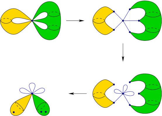
Figure 1. An illustration of the homotopy equivalences used to convert an arbitrary $2$-complex into a wedge product of circles and link-connected $2$-complexes.

A corollary of Theorem 3.1 is that every group that does split as a non-trivial free product is the fundamental group of a link-connected $2$-complex. We conclude this short section with a concrete illustration of the proof.

Example 3.2 (Splitting $2$-complexes).

Let $X$ be the quotient of two disjoint $2$-spheres that identifies two distinct points in the first $2$-sphere and three distinct points in the second $2$-sphere to a single point. The quotient $X$ can be given a cell structure so that it is a standard $2$-complex, but the exact cell structure is irrelevant. The link of the unique vertex $\ast$ in $X$ has $5$ connected components and $X\setminus\{\ast\}$ has $2$. In other words $|I|=5$ and $|J|=2$. Figure 1 illustrates the sequence of steps used to show that $X$ is homotopy equivalent to $\mathbb{S}^{2}\vee\mathbb{S}^{2}\vee\mathbb{S}^{1}\vee\mathbb{S}^{1}\vee\mathbb{S}^{1}$.

4. Torus knots

Having established properties of link-connected $2$-complexes and their combinatorial descriptions, we now turn our attention to examples that illustrate the benefits of using multi-vertex $2$-complexes. We begin with torus knots and torus knot groups.

Definition 4.1 (Torus knots).

The $3$-sphere has a standard genus one Heegaard splitting into two solid tori with a common torus boundary and any simple closed curve that embeds in this common torus is called a torus knot. The essential curves on this torus that bound discs in one solid torus or the other provide a canonical basis for the first homology of the torus and torus knots can be classified by the element of first homology they represent. In particular, for every relatively prime pair of integers $p$ and $q$ there is a knot $K$ called a $(p,q)$-torus knot corresponding to a $(p,q)$-curve on this separating torus. The fundamental group of the complement of $K$ is the corresponding torus knot group $\textsc{Tor}(p,q)$ and a presentation of this group is $\langle a,b\mid a^{p}=b^{q}\rangle$. Although torus knots are only defined when $p$ and $q$ be relatively prime, the presentation makes sense for arbitrary pairs of integers $m$ and $n$ and we extend the definition of $\textsc{Tor}(m,n)$ accoringly.

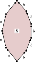
Figure 2. The $2$-cell on the left attached to the graph on the left and the $2$-cell on the right attached to the graph on the right are both $2$-complexes with fundamental group $\textsc{Tor}(4,5)$. Contracting the edge $t$ shows that the two spaces are homotopy equivalent.

Let $X=X_{m,n}$ be the standard $2$-complex of the standard presentation of $\textsc{Tor}(m,n)$, i.e. $\langle a,b\mid a^{m}=b^{n}\rangle$. Although the presentation of a torus knot group is extremely simple, the global structure of the universal cover of $X$ is not immediately obvious. The situation is much clearer if we consider the two vertex $2$-complex $Y=Y_{m,n}$ corresponding to the combinatorial description $[a^{m}t=tb^{n}]$. The $2$-cells and the underlying graphs of the complexes $X_{4,5}$ and $Y_{4,5}$ are depicted in Figure 2. That $X$ and $Y$ are two $2$-complexes with the same fundamental group is clear since the edge labeled $t$ in $Y$ is always embedded and contracting it to a point yields $X$.

As mentioned above, the main benefit of using $Y$ instead of $X$ as a space with fundmamental group $\textsc{Tor}(m,n)$ is that the universal cover of $Y$ is much easier to visualize in its entirety. First add a metric to the polygon used to construct $Y$. As is hinted in Figure 2, we turn it into a metric rectangle with right angles at the four endpoints of the two edges labeled $t$ and with no other sharp corners. To make the edge lengths match up, we make the $a$ edges length $n$ and the $b$ edges length $m$. In the universal cover, these rectangles glue together along the $t$-edges to produce vertical strips that are in turn glued together in a tree-like fashion. In fact, the universal cover $\widetilde{Y}$ can be described as a metric direct product of a tree $T$ and a copy of the real line $\mathbb{R}$. See Figure 3. If we let $K=K_{m,n}$ denote the complete bipartite graph with $m$ vertices of one type and $n$ vertices of the other type, then the tree $T$ is the universal cover of $K$. In particular, $T$ is biregular in that every vertex has valence $m$ or $n$ and every edge connects a vertex of valence $m$ to a vertex of valence $n$. As usual with covering spaces, the group $\textsc{Tor}(m,n)$ acts freely and cocompactly by isometries on the metric space $\widetilde{Y}=T\times\mathbb{R}$, which is contractible and non-positively curved. Using the action of $\textsc{Tor}(m,n)$ on this space it is straightforward to establish the following elementary properties of torus knot groups.

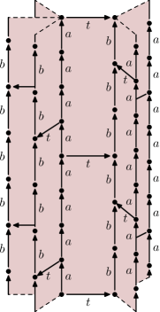
Figure 3. A portion of the universal cover of $Y_{4,3}$.

Theorem 4.2 (Torus knot groups).

If $G=\textsc{Tor}(m,n)$ is a torus knot group for positive integers $m$ and $n$ then: (1) the center of $G$ is infinite cyclic generated by the element $a^{m}=b^{n}$; (2) $G$ is virtually a direct product of a free group and an infinite cyclic group; (3) every nontrivial reduced word equivalent to the identity in $G$ contains a subword equal to $a^{m}$ or $b^{n}$ or their inverses; and finally, (4) every word equivalent to the identity in $G$ can be reduced to the identity by iteratively replacing $a^{m}$ with $b^{n}$, replacing $b^{n}$ with $a^{m}$, and performing free reductions.

Proof Sketch.

Since the listed properties are relatively elementary and they follow fairly quickly once the geometry of $\widetilde{Y}$ and action of $G$ is understood, we merely sketch the proofs. First note that because contracting the edge labeled $t$ in $Y$ yields $X$, contracting the disjoint edges labeled $t$ in $\widetilde{Y}$ yields $\widetilde{X}$. Thus, if we treat the edges labeled $t$ in $\widetilde{Y}$ as though they were contracted (without actually contracting them) we can work with the geometrically pleasing $1$-skeleton of $\widetilde{Y}$ to establish results about the $1$-skeleton of $\widetilde{X}$, i.e. the Cayley graph of $G$ with respect to the generating set $\{a,b\}$. For example, in $X$, the edges labeled $a$ and $b$ label loops which represent elements of the fundamental group, and as such they act on $\widetilde{X}$ by deck transformations once we have chosen a vertex in $\widetilde{X}$ as our base vertex. Thus they also represent actions on $\widetilde{Y}$ by deck transformations once we have chosen an edge labeled $t$ as our base edge.

Fix such an edge $t$ and consider the column labeled with $a$’s at one endpoint, the column labeled with $b$’s at the other and the vertical strip between them. The deck transformation corresponding to the generator $a$ shifts this $a$ column vertically and spins the rest of $\widetilde{Y}$ around this column. After $m$ such motions the entire complex $\widetilde{Y}$ merely experiences a vertical shift. Similarly, the deck transformation corresponding to the generator $b$ shifts this $b$ column vertically and spins the rest of $\widetilde{Y}$ around this column. After $n$ such motions the entire complex $\widetilde{Y}$ merely experiences a vertical shift. From these motions one can show that the only words that commute with $a$ correspond to paths that start at the basic $t$ edge and end at another $t$ edge with an endpoint on this $a$ column. Similarly, any word that commutes with $b$ must correspond to a path that starts at the basic $t$ edge and ends at another $t$ edge with an endpoint on this $b$ column. Thus, the only words that might be central are those that correspond to a path that starts at the basic $t$ edge and ends at another $t$ edge in the same vertical strip. As all these words represent rigid vertical shifts and are powers of the basic vertical shift represented by $a^{m}=b^{n}$, the infinite cyclic subgroup generated by this element is precisely the center of $G$.

To see (2) we note that there is a finite-sheeted cover of $Y$ obtained by identifying edges labeled $t$ in $\widetilde{Y}$ when they belong to the same vertical strip and also identifying two vertical strips if they have their $t$ edges at the same set of heights. We then make the minimal additional identifications necessary for the result to be a covering of $Y$. Geometrically the result is a direct product $K_{m,n}\times\mathbb{S}^{1}$ with fundamental group $\mathbb{F}\times\mathbb{Z}$ where $\mathbb{F}$ is the free group $\pi_{1}(K_{m,n})$ and since the cover is finite-sheeted, the subgroup this represents is finite index.

Next, recall that a syllable of a word is a maximum subword that merely repeats the same letter. For example, the word $a^{5}b^{2}C^{4}$ has $3$ syllables: $a^{5}$, $b^{2}$, and $C^{4}$ (i.e. $c^{-4}$). For (3) we convert a reduced word equivalent to the identity into a closed immeresed path in the $1$-skeleton of $\widetilde{X}$ starting at its base vertex and then finally to a closed immersed path in the $1$-skeleton of $\widetilde{Y}$ by traversing $t$ edges when necessary in order to continue (which occurs precisely at the breaks between syllables). Given such a path, we can look at its projection into the tree $T$. The projection cannot be trivial since there are no closed immersed paths that remain in a single $a$ column or a single $b$ column. Also, the projected curve cannot remain immersed since $T$ is a tree. Thus there is a point in the projected curve where it crosses an edge of $T$ and then immediately backtracks across the same edge. If we consider the portion of the path in $\widetilde{Y}$ that produces this behavior, we see a path that crosses a $t$ edge, travels up or down an $a$ column (or $b$ column) and then crosses back across a $t$ edge in the same vertical strip. Since the path in $\widetilde{Y}$ is immersed, the two $t$ edges must be distinct and the portion between them must contain $a^{m}$, $b^{n}$ or their inverses. Actually this shows more than is claimed in the statement of the theorem. Every reduced word equivalent to the identity in $G$ contains a syllable of the form $a^{k}$ where $k$ is a multiple of $m$ or $b^{\ell}$ where $\ell$ is a multiple of $n$.

Finally, to prove (4) we use the projection of the closed curve to $T$ described above and systematically use the relation $a^{m}=b^{n}$ to shrink the number of edges that the projection crosses in $T$. We should also note that with the lengths as assigned, this results in a nonlength increasing solution for the word problem of the torus knot group $G$. ∎

We conclude our discussion of torus knot groups by noting that in addition to being easier to visualize, the geometry of $Y=Y_{p,q}$ is more closely tied to the geometry of the corresponding torus knot.

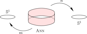
Figure 4. If an annulus has its boundary cycles attached to two different circles with winding numbers $m$ and $n$, respectively, then the fundamental group of the resulting complex is the torus knot group $\textsc{Tor}(m,n)$.

Remark 4.3 (Torus knots and the complex $Y$).

Let $p$ and $q$ be relatively prime integers. There is a natural embedding of $Y=Y_{p,q}$ into the complement of the $(p,q)$-torus knot $K$ so that the complement of the knot deformation retracts onto $Y$. We start by noting an alternate description of the space $Y$. Imagine identifying the two edges of the polygon labeled $t$ before performing the other edge identifications. This shows that $Y$ can be also constructed by attaching an annulus to a pair of circles so that one boundary component is attached to one of the circles with winding number $m$ while attaching the other boundary component to the other circle with winding number $n$. The result is homeomorphic to $Y$. See Figure 4. To embed $Y$ into $\mathbb{S}^{3}\setminus K$ we sent the two circles to the core curves running through the centers of the two solid tori. The annulus can then be embedded in $\mathbb{S}^{3}$ and attached to the circles as needed to form $Y$ in such a way that it cuts through the boundary torus in a $(p,q)$-curve that is parallel to but disjoint from the original $(p,q)$-curve $K$. Finally, it is not too difficult to construct an explicit deformation retraction from $\mathbb{S}^{3}\setminus K$ to $Y$.

5. Solvable Baumslag-Solitar groups

Our next family of examples are the solvable Baumslag-Solitar groups. Althought these are groups where the standard $2$-complex adequately encodes their geometry, we include a very brief discussion of their basic properties so that we can can refer to them in the next section.

Definition 5.1 (Baumslag-Solitar groups).

The Baumslag-Solitar group $BS(m,n)$ is the group defined by the presentation $\langle a,t\mid a^{m}t=ta^{n}\rangle$. The similarity between the Baumslag-Solitar group $BS(m,n)$ and the torus knot group $\textsc{Tor}(m,n)$ should be clear. It too can be described as the fundamental group of a space obtained by attached the two boundary cycles to circles with winding numbers $m$ and $n$. The difference is that this time both boundary cycles are attached to the same circle.

A Baumslag-Solitar group is solvable (in the classical sense of that term) iff $m=n$ and this is also the case where the geometry is most pleasing. Let $G=BS(m,m)$ be a solvable Baumslag-Solitar group and let $X$ be the standard $2$-complex of the presentation $\langle a,t\mid a^{m}t=ta^{m}\rangle$. The one polygon involved can be given the structure of a rectangle as before and the universal cover $\widetilde{X}$ has the structure of a tree $T$ cross the reals. The tree $T$ is a uniformly $m$-branching tree. From this structure, one can compute the center of $G$, see that $G$ is virtually free-by-cyclic, solve the word problem in $G$ and establish basic properties of reduced words equal to the identity in $G$. In other words, one can prove a theorem analogous to Theorem 4.2.

6. One-relator Artin groups

Our third family of examples is closely related to the two previous families. Recall that an Artin group is defined by a presentation inspired by Artin’s classical presentation for the braid groups [3, 4]. In particular, they are defined by presentations in which every relation is one of Artin’s relations.

Definition 6.1 (Artin relations and Artin groups).

Let $(a,b)_{m}$ be the word of length $m$ which starts with $a$ and alternates between $a$ and $b$. In symbols $(a,b)_{m}=abab\ldots$ with $m$ letters total. For example $(a,b)_{2}=ab$, $(a,b)_{3}=aba$ and $(a,b)_{4}=abab$. An Artin relation is a relation of the form $(a,b)_{m}=(b,a)_{m}$ with $m>1$. Thus for small values of $m$ we have commutation $ab=ba$, the braid relation $aba=bab$, and $abab=baba$ for $m=4$. An Artin group is a group defined by a presentation in which every relation is an Artin relation and there is at most one Artin relation for every distinct pair of generators.

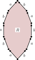
Figure 5. The $2$-cell on the left attached to the graph on the left and the $2$-cell on the right attached to the graph on the right are both $2$-complexes with fundamental group $\textsc{Art}_{5}$. Contracting the edge $t$ shows that the two spaces are homotopy equivalent.

The simplest Artin groups are those with only two generators and one relation. Let $\textsc{Art}_{m}$ denote the one-relator Artin group defined by the presentation $\langle a,b\mid(ab)_{m}=(ba)_{m}\rangle$ and let $X=X_{m}$ be the corresponding standard $2$-complex. As with torus knots, the global structure of the universal cover of $X$ is not immediately clear but there is a homotopy equivalent two-vertex $2$-complex whose universal cover is much easier to visualize. The idea is to replace the Artin relation $(a,b)_{m}=(b,a)_{m}$ with a similar relation that produces a $2$-complex whose $1$-skeleton looks like the lower righthand side of Figure 5. In this graph it is possible to read the word $(a,b)_{m}$ and the word $(b,a)_{m}$ without inserting any $t$ edges, but $t$ edges must be inserted at the two transitions between the two words. Also note that the direction the $t$ edge needs to crossed depends on the parity of $m$. Explicitly, when $m$ is even we consider the combinatorial description $[(a,b)_{m}t=t(b,a)_{m}]$ and when $m$ is odd we consider the combinatorial description $[(a,b)_{m}=t(b,a)_{m}t]$. When these relations are drawn as a rectangle similar to the one shown in Figure 5, the two $t$ edges are pointing in the same direction when $m$ is even and opposite directions when $m$ is odd.

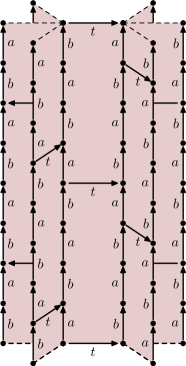
Figure 6. A portion of the universal cover of $Y_{4}$.

In both cases, let $Y=Y_{m}$ denote the corresponding two-vertex $2$-complex. As in our previous examples, the one polygon involved can be given a rectangular metric (with right angles at the endpoints of the two $t$ edges) under which the universal cover $\widetilde{Y}$ is a metric direct product of a uniformly $m$-branching tree $T$ and the reals. A portion of the universal cover for for $Y_{4}$ is shown in Figure 6. From this structure, one can prove a theorem analogous to Theorem 4.2.

Theorem 6.2 (One-relator Artin groups).

If $G=\textsc{Art}_{m}$ is a one-relator Artin group with $m>1$ and $z$ is the element of $G$ represented by $(a,b)_{m}=(b,a)_{m}$ then: (1) the center of $G$ is an infinite cyclic subgroup generated by $z$ when $m$ is even and by $z^{2}$ when $m$ is odd; (2) $G$ is virtually a direct product of a free group and an infinite cyclic group; (3) every nontrivial reduced word equivalent to the identity in $G$ contains a subword equal to $(a,b)_{m}$ or $(b,a)_{m}$ or their inverses; and finally, (4) every word equivalent to the identity in $G$ can be reduced to the identity by iteratively replacing $(a,b)_{m}$ with $(b,a)_{m}$, replacing $(b,a)_{m}$ with $(a,b)_{m}$, and performing free reductions.

Proof Sketch.

The proofs of these properties are nearly identical to the ones given for torus knots and they follow fairly quickly once the geometry of $\widetilde{Y}$ and action of $G$ is understood. First note that because contracting the edge labeled $t$ in $Y$ yields $X$, contracting the disjoint edges labeled $t$ in $\widetilde{Y}$ yields $\widetilde{X}$. Thus, we once again treat the edges labeled $t$ in $\widetilde{Y}$ as though they were contracted (without actually contracting them) allowing us to work with the geometrically pleasing $1$-skeleton of $\widetilde{Y}$ to establish results about the $1$-skeleton of $\widetilde{X}$, i.e. the Cayley graph of $G$ with respect to the generating set $\{a,b\}$. For example, in $X$, the edges labeled $a$ and $b$ label loops which represent elements of the fundamental group, and as such they act on $\widetilde{X}$ by deck transformations once we have chosen a vertex in $\widetilde{X}$ as our base vertex. Thus they also represent actions on $\widetilde{Y}$ by deck transformations once we have chosen an edge labeled $t$ as our base edge. This time though, the deck transformations corresponding to $a$ and $b$ are more complicated. The simple deck transformations are those associated with the words $ab$ and $ba$. One of these stabilizes the column attached to the beginning of our $t$ edge, shifting it up two units while rotating the rest of $\widetilde{Y}$ around this column and the other performs a similar action with respect to the column attached to the other end. After $m$ iterations of the first motion the entire complex experiences a pure vertical shift with no twisting. Similarly after $m$ iterations of the second motion. Any element in the center of $G$ must commute with both of these motions and one can show that the possibilities are words that rigidly vertically shift the vertical strip containing our base $t$ edge. When $m$ is odd, the smallest such shift is represented by $z^{2}=(ab)^{m}=(ba)^{m}$ but when $m$ is even, the word $(a,b)_{m}$ representing $z$, equal to $(ab)^{m/2}$, also represents a rigid vertical shift and in both cases these elements are indeed central in $G$.

To see (2) we construct is a finite-sheeted cover of $Y$ as before. First identify edges labeled $t$ in $\widetilde{Y}$ when they belong to the same vertical strip and are oriented in the same direction, identify two vertical strips if they have their $t$ edges at the same set of heights, and identify columns based on the parity of the heights at which the $a$ edges occur. Geometrically the result is a direct product $\Gamma\times\mathbb{S}^{1}$, where $\Gamma$ is a finite graph with two vertices and $m$ edges connecting them. Thus its fundamental group $\mathbb{F}\times\mathbb{Z}$ where $\mathbb{F}$ is a free group of rank $m-1$ and since the cover is finite-sheeted, the subgroup this represents is finite index in $G$.

For (3) we convert a reduced word equivalent to the identity into a closed immersed path in the $1$-skeleton of $\widetilde{X}$ starting at its base vertex and then finally to a closed immersed path in the $1$-skeleton of $\widetilde{Y}$ by traversing $t$ edges when necessary in order to continue. Given such a path, we can look at its projection into the tree $T$. The projection cannot be trivial since there are no closed immersed paths that remain in a single column and the projected curve cannot remain immersed since $T$ is a tree. Thus there is a point in the projected curve where it crosses an edge of $T$ and then immediately backtracks across the same edge. If we consider the portion of the path in $\widetilde{Y}$ that produces this behavior, we see a path that crosses a $t$ edge, travels up or down a column and then crosses back across a $t$ edge in the same vertical strip. Since the path in $\widetilde{Y}$ is immersed, the two $t$ edges must be distinct and the portion between them must contain $(a,b)_{m}$, $(b,a)_{m}$ or their inverses.

Finally, to prove (4) we use the projection of the closed curve to $T$ described above and systematically use the relation $(a,b)_{m}=(b,a)_{m}$ to shrink the number of edges that the projection crosses in $T$ and note that this results in a nonlength increasing solution for the word problem of $G$. ∎

The fact that one-relator Artin groups have properties similar to torus knot groups and solvable Baumslag-Solitar groups is not accidental.

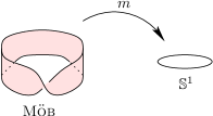
Figure 7. A Möbius band attached to a circle.

Remark 6.3 (Relations with previous examples).

Let $G$ be the one-relator Artin group $\textsc{Art}_{m}$ and let $Y$ be the corresponding two-vertex complex described above with fundamental group $G$. If we identify the two edges labeled $t$ before carrying out the other identifications, we can reanalyze $Y$, depending on the parity of $m$, as either a solvable Baumslag-Solitar group or a torus knot group. More specifically, when $m$ is even, identifying the two $t$ edges creates a torus with boundary cycles attached to the same circle. In particular, the Artin group $\textsc{Art}_{m}$ is isomorphic to solvable Baumslag-Solitar group $BS(m/2,m/2)$ when $m$ is even. On the other hand, when $m$ is odd, identifying the two $t$ edges creates a möbius strip whose boundary cycle is attached to a circle with winding number $m$ (Figure 7). Cutting the möbius strip along its central curve shows that $\textsc{Art}_{m}$ is isomorphic to the torus knot group $\textsc{Tor}(2,m)$ when $m$ is odd.

Note that from a topological perspective, all three classes of groups (torus knot groups, Baumslag-Solitar groups, one-relator Artin groups) are extremely simple as they only involve attaching annuli or möbius strips to one or more circles. It is thus somewhat surprising that they are treated separately and that there does not exist a more uniform set of notations for these groups and their $2$-complexes. Finally, we conclude as promised with a short geometric proof of a key lemma used by Kenneth Appel and Paul Schupp in their investigation of Artin groups of large and extra-large type.

Definition 6.4 (Large type and extra large type).

As mentioned earlier, an Artin group is a group $G$ defined by a presentation in which every relation is an Artin relation $(a,b)_{m}=(b,a)_{m}$ and for every pair of generators there is at most one such relation. If for every relation in the presentation, the integer $m$ is at least $3$ then $G$ is an Artin group of large type and if every integer $m$ is at least $4$ then $G$ is an Artin group of extra large type.

In order to analyze large and extra-large Artin groups using small cancellation theory, they first needed to prove a key intermediate result specifically about one-relator Artin groups. In particular, Appel and Schupp used a detailed inductive analysis of possible van Kampen diagrams in order to establish the follow result that occurs as Lemma $6$ in [2].

Proposition 6.5 (Syllable counts).

Every nontrivial cyclically reduced word that is equal to the identity in $\textsc{Art}_{m}$ contains at least $2m$ syllables.

Proof.

Let $G$ be $\textsc{Art}_{m}$, let $X$ be standard $2$-complex and let $Y$ be the two-vertex complex with fundamental group $G$ described above. The proof proceeds by counting breaks between syllables using the vertical projection from $Y$ to the tree $T$ and the horizontal projection from $Y$ to the real line $\mathbb{R}$. As in the proof of Theorem 6.2, we lift the nontrivial cyclically reduced word equal to the identity in $G$ to an immersed loop in the universal cover $\widetilde{X}$ and then to an immersed loop in the universal cover $\widetilde{Y}$. As argued above, the projection to $T$ is nontrivial and no longer immersed. Moreover, each time the projection to $T$ crosses an edge and immediately recrosses it in the other direction, we can find a copy of the word $(a,b)_{m}$ or $(b,a)_{m}$ in $\widetilde{Y}$ and each such occurence includes $(m-1)$ syllable breaks, i.e. gaps between letters with distinct generators on either side. Since any nontrivial path in a tree includes at least two such backtracks, we have found $2(m-1)=2m-2$ syllable breaks. The final two syllable breaks are located by projecting horizontally to the real line. The path in $\widetilde{Y}$ projects to a path moving up and down the real line. Because it is a closed loop, it attains a maximum and a minimum value. When the path reaches its maximum value it must change columns in $\widetilde{Y}$ (i.e. it must cross a $t$ edge) before continuing back down since the path in $\widetilde{Y}$ is immersed. This leads to a subword of the form $aB$ or $bA$ and to a syllable break that was not previously counted. Similarly local minima in the projection lead to subwords of the form $Ab$ or $Ba$ and to a final syllable break that was not previous counted. Because the closed path has at least $2(m-1)+2=2m$ syllable breaks, it must contain at least $2m$ syllables. ∎

In [2] Appel and Schupp used this result to analyze Artin groups of extra-large type and in [1] Appel extended the analysis to Artin groups of large type. Roughly speaking, if you consider van Kampen diagrams over Artin groups of with respect to an infinite presentation that includes every nontrivial cyclically reduced word in a subgroup generated by two of its generators, then the one can alway find a diagram where no two cells sharing an edge have boundary cycles from the same two generator subgroup. Under these conditions, the overlap between two cells consists of a single letter and thus lives within a single syllable of the boundary word of the either cell. The large or extra-large condition, combined with Proposition 6.5 means that these diagrams satisfy the small cancellation conditions $C(6)$ or $C(8)$, respectively. Once the tools of small cancellation theory are available, they are then able to establish many foundational results for large and extra-large Artin groups. In their original paper Appel and Schupp needed to work a bit to establish Proposition 6.5. The geometry of $Y$ makes this proposition much more transparent.

References

- [1] Kenneth I. Appel. On Artin groups and Coxeter groups of large type. In Contributions to group theory, volume 33 of Contemp. Math., pages 50–78. Amer. Math. Soc., Providence, RI, 1984.
- [2] Kenneth I. Appel and Paul E. Schupp. Artin groups and infinite Coxeter groups. Invent. Math., 72(2):201–220, 1983.
- [3] Emil Artin. Theorie der zöpfe. Hamburg Abh., 4:539–549, 1926.
- [4] Emil Artin. Theory of braids. Ann. of Math. (2), 48:101–126, 1947.