Braids, posets and orthoschemes

Abstract.

In this article we study the curvature properties of the order complex of a graded poset under a metric that we call the “orthoscheme metric”. In addition to other results, we characterize which rank $4$ posets have $\text{{CAT}}(0)$ orthoscheme complexes and by applying this theorem to standard posets and complexes associated with four-generator Artin groups, we are able to show that the $5$-string braid group is the fundamental group of a compact nonpositively curved space.

Barycentric subdivision subdivides an $n$-cube into isometric metric simplices called orthoschemes. We use orthoschemes to turn the order complex of a graded poset $P$ into a piecewise Euclidean complex $K$ that we call its orthoscheme complex. Our goal is to investigate the way that combinatorial properties of $P$ interact with curvature properties of $K$. More specifically, we focus on combinatorial configurations in $P$ that we call spindles and conjecture that they are the only obstructions to $K$ being $\text{{CAT}}(0)$.

Poset Curvature Conjecture.

The orthoscheme complex of a bounded graded poset $P$ is $\text{{CAT}}(0)$ iff $P$ has no short spindles.

One way to view this conjecture is as an attempt to extend to a broader context the flag condition that tests whether a cube complex is $\text{{CAT}}(0)$. We highlight this perspective in §7. Our main theorem establishes the conjecture for posets of low rank.

Theorem A.

The orthoscheme complex of a bounded graded poset $P$ of rank at most $4$ is $\text{{CAT}}(0)$ iff $P$ has no short spindles.

Using Theorem A, we prove that the $5$-string braid group, also known as the Artin group of type $A_{4}$, is a $\text{{CAT}}(0)$ group. More precisely, we prove the following.

Theorem B.

Let $K$ be the Eilenberg-MacLane space for a four-generator Artin group of finite type built from the corresponding poset of $W$-noncrossing partitions and endowed with the orthoscheme metric. When the group is of type $A_{4}$ or $B_{4}$, the complex $K$ is $\text{{CAT}}(0)$ and the group is a $\text{{CAT}}(0)$ group. When the group is of type $D_{4}$, $F_{4}$ or $H_{4}$, the complex $K$ is not $\text{{CAT}}(0)$.

The article is structured as follows. The initial sections recall basic results about posets, complexes and curvature, followed by sections establishing the key properties of orthoschemes, orthoscheme complexes and spindles. The final sections prove our main results and contain some concluding remarks.

1. Posets

We begin with elementary definitions and results about posets. For additional background see [2] or [12].

Definition 1.1 (Poset).

A poset is a set with a fixed implicit reflexive, anti-symmetric and transitive relation $\leq$. A chain is any totally ordered subset, subsets of chains are subchains and a maximal chain is one that is not a proper subchain of any other chain. A chain with $n+1$ elements has length $n$ and its elements can be labeled so that $x_{0}<x_{1}<\cdots<x_{n}$. A poset is bounded below, bounded above, or bounded if it has a minimum element $\mathbf{0}$, a maximum element $\mathbf{1}$, or both. The elements $\mathbf{0}$ and $\mathbf{1}$ are necessarily unique when they exist. A poset has rank $n$ if it is bounded, every chain is a subchain of a maximal chain and all maximal chains have length $n$.

Definition 1.2 (Interval).

For $x\leq y$ in a poset $P$, the interval between $x$ and $y$ is the restriction of the poset to those elements $z$ with $x\leq z\leq y$ and it is denoted by $P(x,y)$ or $P_{xy}$. If every interval in $P$ has a rank, then $P$ is graded. Let $x$ be an element in a graded poset $P$. When $P$ is bounded below, the rank of $x$ is the rank of the interval $P_{\mathbf{0}x}$ and when $P$ is bounded above, the corank of $x$ is the rank of the interval $P_{x\mathbf{1}}$. In general, if every interval in a poset $P$ has a particular property, we say $P$ locally has that property.

Note that a poset is bounded and graded iff it has rank $n$ for some $n$, and that the rank of an element $x$ in a bounded graded poset is the same as the subscript $x$ receives when it is viewed as an element of a maximal chain from $\mathbf{0}$ to $\mathbf{1}$ whose elements are labelled as described above.

Definition 1.3 (Lattice).

Let $x$ and $y$ be elements in a poset $P$. An upper bound for $x$ and $y$ is any element $z$ such that $x\leq z$ and $y\leq z$. The minimal elements among the collection of upper bounds for $x$ and $y$ are called minimal upper bounds of $x$ and $y$. When only one minimal upper bound exists, it is the join of $x$ and $y$ and denoted $x\vee y$. The definitions of lower bounds and maximal lower bounds of $x$ and $y$ are similar. When only one maximal lower bound exists, it is the meet of $x$ and $y$ and denoted $x\wedge y$. A poset in which $x\vee y$ and $x\wedge y$ always exist is called a lattice.

For later use we define a particular configuration that is present in every bounded graded poset that is not a lattice.

Definition 1.4 (Bowtie).

We say that a poset $P$ contains a bowtie if there exist distinct elements $a$, $b$, $c$ and $d$ such that $a$ and $c$ are minimal upper bounds for $b$ and $d$ and $b$ and $d$ are maximal lower bounds for $a$ and $c$. In particular, there is a zig-zag path from $a$ down to $b$ up to $c$ down to $d$ and back up to $a$. An example is shown in Figure 1.

Figure 1. A bounded graded poset that is not a lattice.

Proposition 1.5 (Lattice or bowtie).

A bounded graded poset $P$ is a lattice iff $P$ contains no bowties.

Proof.

If $P$ contains a bowtie, then $b$ and $d$ have no join and $P$ is not a lattice. In the other direction, suppose $P$ is not a lattice because $x$ and $y$ have no join. An upper bound exists because $P$ is bounded, and a minimal upper bound exists because $P$ is graded. Thus $x$ and $y$ must have more than one minimal upper bound. Let $a$ and $c$ be two such minimal upper bounds and note that $x$ and $y$ are lower bounds for $a$ and $c$. If $b$ is a maximal lower bound of $a$ and $c$ satisfying $b\geq x$ and $d$ is a maximal lower bound of $a$ and $c$ satisfying $d\geq y$, then $a$, $b$, $c$, $d$ form a bowtie. We know that $a$ and $c$ are minimal upper bounds of $b$ and $d$ and that $b$ and $d$ are distinct since either failure would create an upper bound of $x$ and $y$ that contradicts the minimality of $a$ and $c$. When $x$ and $y$ have no meet, the proof is analogous. ∎

Posets can be used to construct simplicial complexes.

Definition 1.6 (Order complex).

The order complex of a poset $P$ is a simplicial complex $\lvert P\rvert$ constructed as follows. There is a vertex $v_{x}$ in $\lvert P\rvert$ for every $x\in P$, an edge $e_{xy}$ for all $x<y$ and more generally there is a $k$-simplex in $\lvert P\rvert$ with vertex set $\{v_{x_{0}},v_{x_{1}},\ldots,v_{x_{k}}\}$ for every finite chain $x_{0}<x_{1}<\cdots<x_{k}$ in $P$. When $P$ is bounded, $v_{\mathbf{0}}$ and $v_{\mathbf{1}}$ are the endpoints of $\lvert P\rvert$, and the edge $e_{\mathbf{0}\mathbf{1}}$ connecting them is its diagonal.

The order complex of the poset shown in Figure 1 has $6$ vertices, $13$ edges, $12$ triangles and $4$ tetrahedra. Since every maximal chain contains $\mathbf{0}$ and $\mathbf{1}$, all four tetrahedra contain the diagonal $e_{\mathbf{0}\mathbf{1}}$.

Proposition 1.7 (Contractible).

If a poset is bounded below or bounded above, then its order complex is contractible.

Proof.

If $x$ is an extremum of $P$, then $\lvert P\rvert$ is a topological cone over the complex $\lvert P\setminus\{x\}\rvert$ with $v_{x}$ as the apex of the cone. ∎

2. Complexes

Next we review the theory of piecewise Euclidean and piecewise spherical cell complexes built out of Euclidean or spherical polytopes, respectively. For further background on polytopes see [13] and for polytopal complexes see [7].

Definition 2.1 (Euclidean polytope).

A Euclidean polytope is a bounded intersection of a finite collection of closed half-spaces of a Euclidean space, or, equivalently, it is the convex hull of a finite set of points. A proper face is a nonempty subset that lies in the boundary of a closed half-space containing the entire polytope. Every proper face of a polytope is itself a polytope. In addition there are two trivial faces: the empty face $\emptyset$ and the polytope itself. The interior of a face is the collection of its points that do not belong to a proper subface, and every polytope is a disjoint union of the interiors of its faces. The dimension of a face is the dimension of the smallest affine subspace that containing it. A $0$-dimensional face is a vertex and a $1$-dimensional face is an edge.

Definition 2.2 (PE complex).

A piecewise Euclidean complex (or PE complex) is the regular cell complex that results when a disjoint union of Euclidean polytopes are glued together via isometric identifications of their faces. For simplicity we usually insist that every polytope involved in the construction embeds into the quotient and that the intersection of any two polytopes be a face of each. If there are only finitely many isometry types of polytopes used in the construction, we say it is a complex with finite shapes.

A basic result due to Bridson is that a PE complex with finite shapes is a geodesic metric space, i.e. the distance between two points in the quotient is well-defined and achieved by a path of that length connecting them. This was a key result from Bridson’s thesis [6] and is the main theorem of Chapter I.7 in [7].

The PE complexes built out of cubes deserve special attention.

Example 2.3 (Cube complexes).

A cube complex is a (connected) PE complex $K$ in which every cell used in its construction is isometric to a metric cube of some dimension. Although it is traditional to use cubes with unit length sides, this is not strictly necessary. The fact that faces of $K$ are identified by isometries, together with connectivity, does, however, imply that every edge has the same length and thus $K$ is a rescaled version of a unit cube complex.

In the same way that every poset has an associated cell complex, every regular cell complex has an associated poset.

Definition 2.4 (Face posets).

Every regular cell complex $K$, such as a PE complex, has an associated face poset $P$ with one element $x_{\sigma}$ for each cell $\sigma$ in $K$ ordered by inclusion, that is $x_{\sigma}\leq x_{\tau}$ iff $\sigma\subset\tau$ in $K$. As is well-known, the operations of taking the face poset of a cell complex and constructing the order complex of a poset are nearly but not quite inverses of each other. More specifically, the the order complex of the face poset of a regular cell complex is a topological space homeomorphic to original cell complex but with a different cell structure. The new cells are obtained by barycentrically subdividing the old cells.

Definition 2.5 (Euclidean product).

Let $K$ and $L$ be PE complexes. The metric on the product complex $K\times L$ is defined in the natural way: if the distance in $K$ between $x$ and $x^{\prime}$ is $d_{K}$ and the distance in $L$ between $y$ and $y^{\prime}$ is $d_{L}$, then the distance between $(x,y)$ and $(x^{\prime},y^{\prime})$ is $\sqrt{(d_{K})^{2}+(d_{L})^{2}}$. It is itself a PE complex built out of products of polytopes. More precisely, if $\sigma$ is a nonempty cell in $K$ and $\tau$ is a nonempty cell in $L$, then there is a polytope $\sigma\times\tau$ in $K\times L$. Conversely, every nonempty cell in $K\times L$ is a polytope of this form.

Euclidean polytopes and PE complexes have spherical analogs.

Definition 2.6 (Spherical polytope).

A spherical polytope is an intersection of a finite collection of closed hemispheres in $\mathbb{S}^{n}$, or, equivalently, the convex hull of a finite set of points in $\mathbb{S}^{n}$. In both cases there is an additional requirement that the intersection or convex hull be contained in some open hemisphere of $\mathbb{S}^{n}$. This avoids antipodal points and the non-uniqueness of the geodesics connecting them. With closed hemispheres replacing closed half-spaces and lower dimensional unit subspheres replacing affine subspaces, the other definitions are unchanged.

Definition 2.7 (PS complex).

A piecewise spherical complex (or PS complex) is the regular cell complex that results when a disjoint union of spherical polytopes are glued together via isometric identifications of their faces. As above we usually insist that each polytope embeds into the quotient and that they intersect along faces. As above, so long as the complex has finite shapes, the result is a geodesic metric space.

Definition 2.8 (Vertex links).

Let $v$ be a vertex of a Euclidean polytope $\sigma$. The link of $v$ in $\sigma$ is the set of directions that remain in $\sigma$. More precisely, the vertex link $\text{{lk}}(v,\sigma)$ is the spherical polytope of unit vectors $u$ such that $v+\epsilon u$ is in $\sigma$ for some $\epsilon>0$. More generally, let $v$ be a vertex of a PE complex $K$. The link of $v$ in $K$, denoted $\text{{lk}}(v,K)$ is obtained by gluing together the spherical polytopes $\text{{lk}}(v,\sigma)$ where $\sigma$ is a Euclidean polytope in $K$ with $v$ as a vertex. The intuition is that $\text{{lk}}(v,K)$ is a rescaled version of the boundary of an $\epsilon$-neighborhood of $v$ in $K$.

A vertex link of a Euclidean polytope is a spherical polytope, a vertex link of a PE complex is a PS complex, and a vertex link of a cube complex is a simplicial complex. The converse is also true in the sense that every spherical polytope is a vertex link of some Euclidean polytope, every PS complex is a vertex link of some PE complex, and every simplicial complex is a vertex link of some cube complex.

Definition 2.9 (Spherical joins).

Given PS complexes $K$ and $L$, we define a new PS complex $K\ast L$ that is the spherical analog of Euclidean product. As remarked above, there is a PE complex $K^{\prime}$ with a vertex $v$ such that $K=\text{{lk}}(v,K^{\prime})$ and a PE complex $L^{\prime}$ with a vertex $w$ such that $L=\text{{lk}}(w,L^{\prime})$. We define $K\ast L$ to be the link of $(v,w)$ in $K^{\prime}\times L^{\prime}$. The cell structure of $K\ast L$ as a PS complex is built from spherical joins of cells of $K$ with $L$. In particular, each spherical polytope in $K\ast L$ is $\sigma\ast\tau$ where $\sigma$ is a cell of $K$ and $\tau$ is a cell of $L$. One difference in the spherical context is that the empty face plays an important role. There are cells in $K\ast L$ of the form $\sigma\ast\emptyset$ and $\emptyset\ast\tau$ that fit together to form a copy of $K$ and a copy of $L$, respectively. What is going on is that the link of $(v,w)$ in $K^{\prime}\times\{w\}=K^{\prime}$ is $K\ast\emptyset=K$ and the link of $(v,w)$ in $\{v\}\times L^{\prime}=L^{\prime}$ is $\emptyset\ast L=L$. The spherical join $K\ast L$ can alternatively be defined as the smallest PS complex containing a copy of $K$ and a copy of $L$ such that every point of $K$ is distance $\frac{\pi}{2}$ from every point of $L$ [7, p.63]. Spherical join is a commutative and associative operation on PS complexes with the empty complex $\emptyset$ as its identity.

Next we extend the notion of a vertex link to the link of a face of a polytope and the link of a cell in a PE complex.

Definition 2.10 (Face links).

Let $x$ be a point in an $n$-dimensional Euclidean polytope $\sigma$, let $\tau$ be the unique face of $\sigma$ that contains $x$ in its interior, let $k$ be the dimension of $\tau$, and define $\text{{lk}}(x,\sigma)$ as in Definition 2.8. If $x$ is not a vertex, then $\text{{lk}}(x,\sigma)$ is not a spherical polytope. In fact, $\text{{lk}}(x,\sigma)\supset\text{{lk}}(x,\tau)=\mathbb{S}^{k-1}$ which contains antipodal points since $k>0$. To remedy this situation we note that $\text{{lk}}(x,\sigma)=\text{{lk}}(x,\tau)\ast\text{{lk}}(\tau,\sigma)$ where the latter is a spherical polytope defined as follows. The link of $\tau$ in $\sigma$ is the set of directions perpendicular to $\tau$ that remain in $\sigma$. More precisely, the face link $\text{{lk}}(\tau,\sigma)$ is the spherical polytope of unit vectors $u$ perpendicular to the affine hull of $\tau$ such that for any $x$ in the interior of $\tau$, $x+\epsilon u$ is in $\sigma$ for some $\epsilon>0$. More generally, let $\tau$ be a cell of a PE complex $K$. The link of $\tau$ in $K$, denoted $\text{{lk}}(\tau,K)$, is obtained by gluing together the spherical polytopes $\text{{lk}}(\tau,\sigma)$ where $\sigma$ is a Euclidean polytope in $K$ with $\tau$ as a face. As an illustration, if $x$ is a point in an edge $\tau$ of a tetrahedron $\sigma$, then $\text{{lk}}(\tau,\sigma)$ is a spherical arc whose length is the size of the dihedral angle between the triangles containing $\tau$, whereas $\text{{lk}}(x,\tau)=\mathbb{S}^{0}$ and $\text{{lk}}(x,\sigma)=\text{{lk}}(x,\tau)\ast\text{{lk}}(\tau,\sigma)=\mathbb{S}^{0}\ast\text{{lk}}(\tau,\sigma)$ is a lune of the $2$-sphere. More generally, if $x$ is a point in a PE complex $K$, $\tau$ is the unique cell of $K$ containing $x$ in its interior, and $k$ is the dimension of $\tau$, then, viewing $\text{{lk}}(x,K)$ as a rescaling of the boundary of an $\epsilon$-neighborhood of $x$ in $K$, we have that $\text{{lk}}(x,K)=\text{{lk}}(x,\tau)\ast\text{{lk}}(\tau,K)=\mathbb{S}^{k-1}\ast\text{{lk}}(\tau,K)$.

Definition 2.11 (Links in PS complexes).

Let $\sigma$ be a cell in a PS complex $K$. To define $\text{{lk}}(\sigma,K)$ we find a PE complex $K^{\prime}$ with vertex $v$ such that $K=\text{{lk}}(v,K^{\prime})$ and then identify the unique cell $\sigma^{\prime}$ in $K^{\prime}$ such that $\sigma=\text{{lk}}(v,\sigma^{\prime})$. We then define the PS complex $\text{{lk}}(\sigma,K)$ as the PS complex $\text{{lk}}(\sigma^{\prime},K^{\prime})$.

We conclude by recording some elementary properties of links and joins.

Proposition 2.12 (Links of links).

If $\sigma\subset\sigma^{\prime}$ are cells in a PE or PS complex $K$ then there is a cell $\tau$ in $L=\text{{lk}}(\sigma,K)$ such that $\text{{lk}}(\tau,L)=\text{{lk}}(\sigma^{\prime},K)$. Moreover, the link of every cell $\tau$ in $\text{{lk}}(\sigma,K)$ arises in this way. In other words, a link of a cell in the link of a cell is a link of a larger cell in the original complex.

Proposition 2.13 (Links of joins).

Let $K$ and $L$ be PS complexes with cells $\sigma$ and $\tau$ respectively. If $K^{\prime}=\text{{lk}}(\sigma,K)$ and $L^{\prime}=\text{{lk}}(\tau,L)$, then $K^{\prime}\ast L$, $K\ast L^{\prime}$ and $K^{\prime}\ast L^{\prime}$ are links of cells in $K\ast L$. Moreover, every link of a cell in $K\ast L$ is of one of these three types.

3. Curvature

As a final bit of background, we review curvature conditions such as $\text{{CAT}}(0)$ and $\text{{CAT}}(1)$. In general these terms are defined by requiring that certain geodesic triangles be “thinner” than comparison triangles in $\mathbb{R}^{2}$ or $\mathbb{S}^{2}$, but because we are just reviewing $\text{{CAT}}(0)$ PE complexes and $\text{{CAT}}(1)$ PS complexes, alternate definitions are available that only involve the existence of short geodesic loops in links of cells.

Definition 3.1 (Geodesics and geodesic loops).

A geodesic in a metric space is an isometric embedding of a metric interval and a geodesic loop is an isometric embedding of a metric circle. A local geodesic and local geodesic loop are weaker notions that only require the image curves be locally length minimizing. For example, a path more than halfway along the equator of a $2$-sphere is a local geodesic but not a geodesic and a loop that travels around the equator twice is a local geodesic loop but not a geodesic loop. A loop in a PS complex of length less than $2\pi$ is called short and a PS complex that contains no short local geodesic loops is called large.

Definition 3.2 (Curvature conditions).

If $K$ is a PE complex with finite shapes and the link of every cell in $K$ is large, then $K$ is nonpositively curved or locally $\text{{CAT}}(0)$. If, in addition, $K$ is connected and simply connected, then $K$ is $\text{{CAT}}(0)$. As a consequence of the general theory of $\text{{CAT}}(0)$ spaces, such a complex $K$ is contractible. If $K$ is a PS complex and the link of every cell in $K$ is large, then $K$ is locally $\text{{CAT}}(1)$. If, in addition, $K$ itself is large, then $K$ is $\text{{CAT}}(1)$.

It follows from the definitions and Proposition 2.12 that a PE complex is nonpositively curved iff its vertex links are $\text{{CAT}}(1)$. Moreover, in the same way that every PS complex is a vertex link of a PE complex, every $\text{{CAT}}(1)$ PS complex is the vertex link of a $\text{{CAT}}(0)$ PE complex.

A standard example where the $\text{{CAT}}(0)$ condition is easy to check is in a cube complex. The link of a cell in a cube complex is a PS simplicial complex built out of all-right spherical simplices, i.e. spherical simplices in which every edge has length $\frac{\pi}{2}$. To check whether a cube complex is $\text{{CAT}}(0)$ it is sufficient to check whether its vertex links satisfy the purely combinatorial condition of being flag complexes.

Definition 3.3 (Flag complexes).

A simplicial complex contains an empty triangle if there are three vertices pairwise joined by edges but no triangle with these three vertices as its corners. More generally, a simplicial complex $K$ contains an empty simplex if for some $n>1$, $K$ contains the boundary of an $n$-simplex but no $n$-simplex with the same vertex set. A flag complex is a simplicial complex with no empty simplices.

Proposition 3.4 ($\text{{CAT}}(0)$ cube complexes).

A cube complex $K$ is $\text{{CAT}}(0)$ iff $\text{{lk}}(v,K)$ is a flag complex for every vertex $v$ which is true iff $\text{{lk}}(\sigma,K)$ has no empty triangles for every cell $\sigma$.

If a PS complex $K$ is locally $\text{{CAT}}(1)$ but not $\text{{CAT}}(1)$ (i.e. the links of $K$ are large, but $K$ itself is not large) then we say $K$ is not quite $\text{{CAT}}(1)$. In [3] Brian Bowditch characterized not quite $\text{{CAT}}(1)$ spaces using the notion of a shrinkable loop.

Definition 3.5 (Shrinkable loop).

Let $\gamma$ be a rectifiable loop of finite length in a metric space. We say that $\gamma$ is shrinkable if there exists a continuous deformation from $\gamma$ to a loop $\gamma^{\prime}$ that proceeds through rectifiable curves of finite length in such a way that the lengths of the intermediate curves are nonincreasing and the length of $\gamma^{\prime}$ is strictly less than the length of $\gamma$. If $\gamma$ is not shrinkable, it is unshrinkable.

The following is a special case of the general results proved in [3].

Lemma 3.6 (Not quite $\text{{CAT}}(1)$).

If $K$ is a locally $\text{{CAT}}(1)$ PS complex with finite shapes, then the following are equivalent:

1. $K$ is not quite $\text{{CAT}}(1)$,

2. $K$ contains a short geodesic loop,

3. $K$ contains a short local geodesic loop, and

4. $K$ contains a short unshrinkable loop.

This is an extremely useful lemma since it is sometimes easier to establish that every loop in a space is shrinkable than it is to show that it does not contain a short local geodesic. Sometimes, for example, a single homotopy shrinks every curve simultaneously.

Definition 3.7 (Monotonic contraction).

Let $X$ be a metric space and let $H:X\times[0,1]\to X$ be a homotopy contracting $X$ to a point (i.e. $H_{0}$ is the identity map and $H_{1}$ is a constant map). We say $H$ is a monotonic contraction if $H$ simultaneously and monotonically shrinks every rectifiable curve in $X$ to a point.

An example of a monotonic contraction is straightline homotopy from the identity map on $\mathbb{R}^{n}$ to a constant map. A spherical version of monotonic contraction is needed in §4.

Definition 3.8 (Hemispheric contraction).

Let $u$ be a point in $\mathbb{S}^{n}$ and let $X$ be a hemisphere of $\mathbb{S}^{n}$ with $u$ as its pole, i.e. the ball of radius $\frac{\pi}{2}$ around $u$. Every point $v$ in $X$ lies on a unique geodesic connecting $v$ to $u$ and we can define a homotopy that moves $v$ to $u$ at a constant speed so that at time $t$ it has traveled $t$ of the distance along this geodesic. This hemispheric contraction to $u$ is a monotonic contraction in the sense defined above.

Although Lemma 3.6 only applies to locally $\text{{CAT}}(1)$ PS complexes, such contexts can always be found when curvature conditions fail.

Proposition 3.9 (Curvature and links).

Let $K$ be a connected and simply-connected PE complex with finite shapes. If $K$ is not $\text{{CAT}}(0)$ then there is a cell $\sigma$ in $K$ such that $\text{{lk}}(\sigma,K)$ is not quite $\text{{CAT}}(1)$. Similarly, if $K$ is a PS complex that is not $\text{{CAT}}(1)$ then either $K$ itself is not quite $\text{{CAT}}(1)$ or there is a cell $\sigma$ such that $\text{{lk}}(\sigma,K)$ is not quite $\text{{CAT}}(1)$.

Proof.

Let $\mathcal{S}$ be the set of the cells $\sigma$ in $K$ such that $\text{{lk}}(\sigma,K)$ is not $\text{{CAT}}(1)$ and order them by inclusion. Unless $K$ itself is a not quite $\text{{CAT}}(1)$ PS complex, the set $\mathcal{S}$ is not empty. Moreover, because $K$ has finite shapes, $K$ is finite dimensional, and $\mathcal{S}$ has maximal elements. If $\sigma$ is such a maximal element, then maximality combined with Proposition 2.12 shows that $\text{{lk}}(\sigma,K)$ is locally $\text{{CAT}}(1)$. Since $\sigma$ is in $\mathcal{S}$, $\text{{lk}}(\sigma,K)$ is not $\text{{CAT}}(1)$. Thus $\text{{lk}}(\sigma,K)$ is not quite $\text{{CAT}}(1)$. ∎

To show that a PE or PS complex is not $\text{{CAT}}(0)$ or $\text{{CAT}}(1)$ it is convenient to be able to construct and detect local geodesic loops. We do this using piecewise geodesics.

Definition 3.10 (Piecewise geodesics).

Let $K$ be a PE or PS complex and let $(x_{0},x_{1},\ldots,x_{n})$ be a sequence of points in $K$ such that for each $i$, $x_{i-1}$ and $x_{i}$ belong to a unique minimal common cell of $K$ and $x_{0}=x_{n}$. The piecewise geodesic loop defined by this list is the concatenation of the unique geodesics from $x_{i-1}$ to $x_{i}$ in the (unique) minimal common cell containing them. The points $x_{i}$ are its transition points. Piecewise geodesics are local geodesics iff they are locally geodesic at its transition points. This can be determined by examining two transition vectors: the unit tangent vector at $x_{i}$ for the geodesic connecting $x_{i}$ to $x_{i+1}$ and the unit tangent vector at $x_{i}$ for the geodesic from $x_{i}$ to $x_{i-1}$ (traversed in reverse). These correspond to two points in $\text{{lk}}(x_{i},K)$. We say that the transition points are far apart if the distance between them is at least $\pi$ inside $\text{{lk}}(x_{i},K)$. Finally, a piecewise geodesic loop $\gamma$ in a PS or PE complex $K$ is a local geodesic iff at every transition point $x$, the transition vectors are far apart in $\text{{lk}}(x,K)$.

We conclude by relating curvature, links and spherical joins.

Proposition 3.11 ($\text{{CAT}}(1)$ and joins).

Let $K$ and $L$ be PS complexes.

1. $K\ast L$ is $\text{{CAT}}(1)$ iff $K$ and $L$ are $\text{{CAT}}(1)$.

2. If $K\ast L$ is locally $\text{{CAT}}(1)$ then $K$ and $L$ are locally $\text{{CAT}}(1)$.

3. If $K\ast L$ is not quite $\text{{CAT}}(1)$ then $K$ or $L$ is not quite $\text{{CAT}}(1)$.

Similar assertions hold for spherical joins of the form $K_{1}\ast K_{2}\ast\cdots\ast K_{n}$.

Proof.

The first part is Corollary II.3.15 in [7]. For the second assertion suppose $K\ast L$ is locally $\text{{CAT}}(1)$ and let $K^{\prime}$ be a link of $K$. Since $K^{\prime}\ast L$ is a link of $K\ast L$ (Proposition 2.13), it is $\text{{CAT}}(1)$ by assumption. But then $K^{\prime}$ is $\text{{CAT}}(1)$ by the part $1$ and $K$ is locally $\text{{CAT}}(1)$. The third part merely combines the first two and extending to multiple joins is an easy induction. ∎

4. Orthoschemes

In this section we introduce the shapes that H.S.M. Coxeter called “orthoschemes” [8] and our main goal is to establish that face links in orthoschemes decompose into simple shapes (Corollary 4.7). Roughly speaking an orthoscheme is the convex hull of a piecewise linear path that proceeds along mutually orthogonal lines.

Definition 4.1 (Orthoschemes).

Let $(v_{0},v_{1},\ldots,v_{n})$ be an ordered list of $n+1$ points in $\mathbb{R}^{n}$ and for each $i\in[n]$ let $u_{i}$ be the vector from $v_{i-1}$ to $v_{i}$. If the vectors $\{u_{i}\}$ form an orthogonal basis of $\mathbb{R}^{n}$ then the convex hull of the points $\{v_{i}\}$ is a metric $n$-simplex called an $n$-orthoscheme that we denote $\textsf{Ortho}(v_{0},\ldots,v_{n})$. If the vectors $\{u_{i}\}$ form an orthonormal basis, then it is a standard $n$-orthoscheme. It follows easily from the definition that every face of an orthoscheme (formed by selecting a subset of its vertices) is itself an orthoscheme, although not all faces of a standard orthoscheme are standard. Faces defined by consecutive vertices are of particular interest and we use $O(i,j)$ to denote the face $\textsf{Ortho}(v_{i},\ldots,v_{j})$ of $O=\textsf{Ortho}(v_{0},\ldots,v_{n})$. The points $v_{i}$ are the vertices of the orthoscheme, $v_{0}$ and $v_{n}$ are its endpoints and the edge connecting $v_{0}$ and $v_{n}$ is its diagonal. A $3$-orthoscheme is shown in Figure 2.

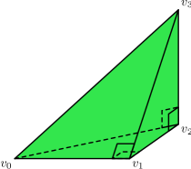
Figure 2. A $3$-dimensional orthoscheme.

For later use we define a contraction of an endpoint link of an orthoscheme.

Proposition 4.2 (Endpoint contraction).

If $v$ is an endpoint of an orthoscheme $O$ and $u$ is the unit vector pointing from $v$ along its diagonal, then hemispheric contraction to $u$ monotonically contracts $\text{{lk}}(v,O)$.

Proof.

Let $O=\textsf{Ortho}(v_{0},\ldots,v_{n})$ and let $v=v_{0}$. Without loss of generality arrange $O$ in $\mathbb{R}^{n}$ so that $v_{0}$ is the origin and each vector $v_{i}-v_{i-1}$ is a positive scalar multiple of a standard basis vector. In this coordinate system all of $O$ lies in the nonnegative orthant and the coordinates of $v_{n}$ are strictly positive. In particular the convex spherical polytope $\text{{lk}}(v,O)$ is contained in an open hemisphere of $\mathbb{S}^{n-1}$ with $u$ as its pole, where $u$ is the unit vector pointing towards $v_{n}$. This is because an all positive vector such as $u$ and any nonzero nonnegative vector have a positive dot product, making the angle between them acute. Finally, hemispheric contraction to $u$ monotonically contracts $\text{{lk}}(v,O)$ because $\text{{lk}}(v,O)$ is a convex set containing $u$. ∎

The orthogonality embedded in the definition of an orthoscheme causes its face links to decompose into spherical joins. As a warm-up for the general statement, we consider links of vertices and edges in orthoschemes.

Example 4.3 (Vertex links in orthoschemes).

Let $O=\textsf{Ortho}(v_{0},v_{1},\ldots,v_{n})$ be an orthoscheme, let $v=v_{k}$ be a vertex with $0<k<n$, and consider suborthoschemes $K=O(0,k)$ and $L=O(k,n)$. The affine subspaces containing $K$ and $L$ are orthogonal to each other and the original orthoscheme is the convex hull of these two faces. Thus $\text{{lk}}(v,O)=\text{{lk}}(v,K)\ast\text{{lk}}(v,L)$. In fact, this formula remains valid when $k=0$ (or $k=n$) since then $K$ (or $L$) has only a single point, its link is empty and this factor drops out of the spherical join since $\emptyset$ is the identity of the spherical join operation. Finally, note that the factors are endpoint links of the suborthoschemes $K$ and $L$.

Example 4.4 (Edge links in orthoschemes).

For each $k\leq\ell$ consider the link of the edge $e_{k\ell}$ connecting $v_{k}$ and $v_{\ell}$ in $O=\textsf{Ortho}(v_{0},v_{1},\ldots,v_{n})$. If we define $K=O(0,k)$, $L=O(k,\ell)$ and $M=O(\ell,n)$ then we claim that $\text{{lk}}(e_{k\ell},O)=\text{{lk}}(v_{k},K)\ast\text{{lk}}(e_{k\ell},L)\ast\text{{lk}}(v_{\ell},M)$. To see this note that the linear subspaces corresponding to the affine spans of $K$, $L$ and $M$ form an orthogonal decomposition of $\mathbb{R}^{n}$ and, as a consequence, any vector can be uniquely decomposed into three orthogonal components. It is then straightforward to see that a vector perpendicular to $e_{k\ell}$ points into $O$ iff its components live in the specified links. The first and last factors are local endpoint links and the middle factor is a local diagonal link. As above, the first factors drops out when $k=0$, the last factor drops out when $\ell=n$, but also note that the middle factor drops out when $k$ and $\ell$ are consecutive since the diagonal link of $O(k,k+1)$ is empty.

We are now ready for the precise general statement.

Proposition 4.5 (Links in orthoschemes).

Let $O=\textsf{Ortho}(v_{0},v_{1},\ldots,v_{n})$ and let $\sigma$ be a $k$-dimensional face with vertices $\{v_{x_{0}},v_{x_{1}},\ldots,v_{x_{k}}\}$ where $0\leq x_{0}<x_{1}<\cdots<x_{k}\leq n$. The link of $\sigma$ in $O$ is a spherical join of two endpoint links and $k$ diagonal links of suborthoschemes. More specifically,

$$\text{{lk}}(\sigma,O)=K_{\mathbf{0}}\ast L_{0}\ast L_{1}\ast\cdots\ast L_{k}\ast K_{\mathbf{1}}$$

where $K_{\mathbf{0}}=\text{{lk}}(v_{x_{0}},O(\mathbf{0},x_{0}))$ and $K_{\mathbf{1}}=\text{{lk}}(v_{x_{k}},O(x_{k},\mathbf{1}))$ are local endpoint links, and each $L_{i}=\text{{lk}}(e_{x_{i-1}x_{i}},O(x_{i-1},x_{i}))$ is a local diagonal link.

Proof.

The full proof is basically the same as the one given above for edge links. Orthogonally decompose $\mathbb{R}^{n}$ into linear subspaces corresponding to the affine hulls of $O(\mathbf{0},x_{0})$, $O(x_{k},\mathbf{1})$ and $O(x_{i-1},x_{i})$ for each $i\in[k]$, then check that a vector perpendicular to $\sigma$ points into $O$ iff its components live in the listed links. In an orthogonal basis compatible with the orthogonal decomposition that contains the local diagonal directions along each $e_{x_{i-1}x_{i}}$ this conclusion is immediate. ∎

Coxeter’s interest in these shapes is related to the observation that the barycentric subdivision of a regular polytope decomposes it into isometric orthoschemes. These orthoschemes are fundamental domains for the action of its isometry group and correspond to the chambers of its Coxeter complex. For example, a barycentric subdivision of the $3$-cube of side length $2$ partitions it into $48$ standard $3$-orthoschemes and the barycentric subdivision of an $n$-cube of side length $2$ produces $n!\cdot 2^{n}$ standard $n$-orthoschemes (see Figure 3). These cube decompositions also make it easy to identify the shape of the endpoint link and the diagonal link in a standard orthoscheme.

Figure 3. Barycentric subdivision of a $3$-cube of side length $2$ into $48$ standard $3$-orthoschemes.

Definition 4.6 (Coxeter shapes).

Let $O=\textsf{Ortho}(v_{0},v_{1},\ldots,v_{n})$ be a standard $n$-orthoscheme. The links $\text{{lk}}(v_{0},O)$ and $\text{{lk}}(v_{n},O)$, are isometric to each other and we call this common shape $\beta_{n}$ because it is a spherical simplex known as the Coxeter shape of type $B_{n}$. The type $B_{n}$ Coxeter group is the isometry group of the $n$-cube and the barycentric subdivision of the $n$-cube mentioned above shows that $\beta_{n}$ is its Coxeter shape, i.e. a fundamental domain for the action of this group on the sphere. In low dimensions, $\beta_{0}=\emptyset$, $\beta_{1}$ is a point, $\beta_{2}$ is an arc of length $\frac{\pi}{4}$ and $\beta_{3}$ is a spherical triangle with angles $\frac{\pi}{2}$, $\frac{\pi}{3}$, and $\frac{\pi}{4}$. Similarly, the link of the diagonal connecting $v_{0}$ and $v_{n}$ in $O$ is a shape that we call $\alpha_{n-1}$ because it is the spherical simplex known as the Coxeter shape of type $A_{n-1}$. The $A_{n-1}$ Coxeter group is the symmetric group $\textsf{Sym}_{n}$, the isometry group of the regular $(n-1)$-simplex and also the stabilizer of a vertex inside the isometry group of the $n$-cube. In low dimensions, $\alpha_{0}=\emptyset$, $\alpha_{1}$ is a point, $\alpha_{2}$ is an arc of length $\frac{\pi}{3}$ and $\alpha_{3}$ is a spherical triangle with angles $\frac{\pi}{2}$, $\frac{\pi}{3}$, and $\frac{\pi}{3}$.

The following corollary of Proposition 4.5 is now immediate.

Corollary 4.7 (Links in standard orthoschemes).

The link of a face of a standard orthoscheme is a spherical join of spherical simplices each of type $A$ or type $B$. More specifically, in the notation of Proposition 4.5, $K_{\mathbf{0}}$ has shape $\beta_{x_{0}}$, $K_{\mathbf{1}}$ has shape $\beta_{n-x_{n}}$ and $L_{i}$ has shape $\alpha_{j}$ with $j=x_{i+1}-x_{i}-1$.

As an illustration, the link of the tetrhedron with corners $v_{3}$, $v_{6}$, $v_{7}$ and $v_{12}$ in a standard $12$-orthoscheme is isometric to $\beta_{3}\ast\alpha_{2}\ast\alpha_{0}\ast\alpha_{4}\ast\beta_{0}=\beta_{3}\ast\alpha_{2}\ast\alpha_{4}$. Finally we record a few results about lengths and angles in orthoscheme links that are needed later in the article.

Proposition 4.8 (Edge lengths).

The link of the diagonal of a standard $n$-orthoscheme $O=\textsf{Ortho}(v_{0},\ldots,v_{n})$ is a spherical simplex of shape $\alpha_{n-1}$ whose vertices correspond to the $v_{i}$ with $0<i<n$. Moreover, if $i$, $j$, and $k$ are positive integers with $i+j+k=n$ and $\theta$ is the length of the edge connecting the vertex of rank $i$ and the vertex of corank $k$ in $\alpha_{n-1}$, then $0<\theta<\frac{\pi}{2}$ and $\cos(\theta)=\sqrt{\frac{i}{i+j}\cdot\frac{k}{j+k}}$.

Proof.

Consider the triangle with vertices $v_{0}$, $v_{i}$ and $v_{n-k}=v_{i+j}$. If we project this triangle onto the hyperplane perpendicular to the edge $e_{0n}$, then the angle at $v_{0}$ in the projected triangle is the length of the corresponding edge in $\alpha_{n-1}$. Let $u$ be the projection of $e_{0i}$ and let $v$ be the projection of $e_{0(n-k)}$ (with both multiplied by $n$ to clear the denominators). In coordinates $u=((j+k)^{i},(-i)^{j+k})$ and $v=(k^{i+j},(-i-j)^{k})$. Here we are using Conway’s exponent notation to simplify vector expressions. In words the first $i$ coordinates of $u$ are $j+k$ and the remaining $j+k$ coordinates are $-i$. The dot products simplify as follows: $u\cdot v=i.k.n$ while $u\cdot u=i.(j+k).n$ and $v\cdot v=(i+j).k.n$. Thus

$$\cos^{2}(\theta)=\frac{(u\cdot v)(u\cdot v)}{(u\cdot u)(v\cdot v)}=\frac{(i.k.n)(i.k.n)}{(i.(j+k).n)((i+j).k.n)}=\frac{i}{i+j}\cdot\frac{k}{j+k}.$$

∎

Corollary 4.9 (Spherical triangles).

Let $\textsf{Ortho}(v_{0},\ldots,v_{n})$ be a standard $n$-orthoscheme. For each $0<x<y<z<n$, the diagonal link of the suborthoscheme $\textsf{Ortho}(v_{0},v_{x},v_{y},v_{z},v_{n})$ is a spherical triangle with acute angles at $v_{x}$ and $v_{z}$ and a right angle at $v_{y}$.

Proof.

From Proposition 4.8 the lengths of the edges of the spherical triangle are known explicitly and the angle assertions follow from the standard spherical trigonometry. For example, if we select positive integers $i+j+k+l=n$ such that $v_{x}$ has rank $i$, $v_{y}$ has rank $i+j$ and $v_{z}$ has rank $i+j+k$, then $\cos\lvert e_{xy}\rvert=\sqrt{\frac{i}{i+j}\cdot\frac{k+l}{j+k+l}}$, $\cos\lvert e_{yz}\rvert=\sqrt{\frac{i+j}{i+j+k}\cdot\frac{l}{k+l}}$ and $\cos\lvert e_{xz}\rvert=\sqrt{\frac{i}{i+j+k}\cdot\frac{l}{j+k+l}}$. From the equality $\cos\lvert e_{xy}\rvert\cdot\cos\lvert e_{yz}\rvert=\cos\lvert e_{xz}\rvert$ and the spherical law of cosines we infer that the angle at $v_{y}$ is a right angle. The acute angle conclusion involves a similar but messier computation. ∎

5. Orthoscheme complexes

In this section we use orthoschemes to turn order complexes into PE complexes. Although every simplicial complex can be turned into a PE complex by making simplices regular and every edge length $1$, the curvature properties of the result tend to be hard to evaluate. For order complexes of graded posets orthoschemes are a better option.

Definition 5.1 (Orthoscheme complex).

The orthoscheme complex of a graded poset $P$ is a metric version of its order complex $\lvert P\rvert$ that assigns every top dimensional simplex in $\lvert P\rvert$ (i.e. those corresponding to maximal chains $x_{0}<x_{1}<\cdots<x_{n}$) the metric of a standard orthoscheme with $v_{x_{i}}$ corresponding to $v_{i}$. As a result, for all elements $x<y$ in $P$, the length of the edge connecting $v_{x}$ and $v_{y}$ in $\lvert P\rvert$ is $\sqrt{k}$ where $k$ is the rank of $P_{xy}$. When $\lvert P\rvert$ is turned into a PE complex in this way we say that $\lvert P\rvert$ is endowed with the orthoscheme metric. Unless otherwise specified, from now on $\lvert P\rvert$ indicates an orthoscheme complex, i.e. an order complex with the orthoscheme metric.

One reason for using this particular metric on the order complex of a poset is that it turns standard examples of posets into metrically interesting PE complexes.

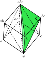
Figure 4. The rank $3$ boolean lattice and its unit $3$-cube orthoscheme complex. The orthoscheme from the chain $\emptyset\subset\{b\}\subset\{b,c\}\subset\{a,b,c\}$ is shaded.

Example 5.2 (Boolean lattices).

The rank $n$ boolean lattice is the poset of all subsets of $[n]:=\{1,2,\ldots,n\}$ ordered by inclusion. The orthoscheme complex of a boolean lattice is a subdivided unit $n$-cube (or one orthant of the barycentric subdivision of the $n$-cube of side length $2$ described earlier), its endpoint link is the barycentric subdivision of an all-right spherical simplex tiled by simplices of shape $\beta_{n}$ and its diagonal link is a subdivided sphere tiled by simplices of shape $\alpha_{n-1}$. See Figure 4.

That the orthoscheme complex of a boolean lattice is a cube can be explained by a more general fact about products.

Remark 5.3 (Products).

A product of posets produces an orthoscheme complex that is a product of metric spaces. In particular, if $P$ and $Q$ are bounded graded posets, then $\lvert P\times Q\rvert$ and $\lvert P\rvert\times\lvert Q\rvert$ are isometric. The product on the left is a product of posets and the product on the right is a product of metric spaces. Since finite boolean lattices are poset products of two element chains, their orthoscheme complexes are, up to isometry, products of unit intervals, i.e. cubes.

Cube complexes produce a second family of examples.

Example 5.4 (Cube complexes).

Let $K$ be a cube complex scaled so that every edge has length $2$. The face poset of $K$ is a graded poset $P$ whose intervals are boolean lattices. The orthoscheme complex $\lvert P\rvert$ is isometric to the cube complex $K$. In other words, the metric barycentric subdivision of an arbitrary cube complex is identical to the orthoscheme complex of its face poset.

A third family of examples shows that there are interesting $\text{{CAT}}(0)$ orthoscheme complexes unrelated to cubes and cube complexes.

Example 5.5 (Linear subspace posets).

The $n$-dimensional linear subspace poset over a field $\mathbb{F}$ is the poset $L_{n}(\mathbb{F})$ of all linear subspaces of the $n$-dimensional vector space $\mathbb{F}^{n}$ ordered by inclusion. It’s basic properties are explored in Chapter $3$ of [12]. The poset $L_{n}(\mathbb{F})$ is bounded above by $\mathbb{F}^{n}$ and below by the trivial subspace and it is graded by the dimension of the subspace an element of $L_{n}(\mathbb{F})$ represents. It turns out that the orthoscheme complex of $L_{n}(\mathbb{F})$ is a $\text{{CAT}}(0)$ space and its diagonal link is a standard example of a thick spherical building of type $A_{n-1}$. The smallest nontrivial example, with $\mathbb{F}=\mathbb{Z}_{2}$ and $n=3$, is illustrated in Figure 5 along with its diagonal link. The middle levels of $L_{3}(\mathbb{Z}_{2})$ correspond to the $7$ points and $7$ lines of the projective plane of order $2$ and its diagonal link is better known as the Heawood graph, or as the incidence graph of the Fano plane.

Figure 5. The poset $L_{3}(\mathbb{Z}_{2})$ and its diagonal link. In the PS complex on the right, every edge in the graph should be viewed as a spherical arc of length $\frac{\pi}{3}$.

With these examples in mind, we now turn to the question of when the orthoscheme complex of a bounded graded poset $P$ is a $\text{{CAT}}(0)$ PE complex. The first step is to examine some of its more elementary links.

Definition 5.6 (Elementary links).

Let $P$ be a bounded graded poset of rank $n$. Three links in the orthoscheme complex $\lvert P\rvert$ are of particular interest. The PS complexes $\text{{lk}}(v_{\mathbf{0}},\lvert P\rvert)$ and $\text{{lk}}(v_{\mathbf{1}},\lvert P\rvert)$ are the endpoint links of $\lvert P\rvert$ and $\text{{lk}}(e_{\mathbf{0}\mathbf{1}},\lvert P\rvert)$ is its diagonal link. The endpoint links are PS complex built out of copies of $\beta_{n}$ and the diagonal link is a PS complex built out of copies of $\alpha_{n-1}$. In fact, $\text{{lk}}(v_{\mathbf{0}},\lvert P\rvert)$ is the simplicial complex $\lvert P\setminus\{\mathbf{0}\}\rvert$ with a PS $\beta_{n}$ metric applied to each maximal simplex. Similarly, $\text{{lk}}(e_{\mathbf{0}\mathbf{1}},\lvert P\rvert)$ is $\lvert P\setminus\{\mathbf{0},\mathbf{1}\}\rvert$ with an $\alpha_{n-1}$ metric on each maximal simplex. Collectively these three links are the elementary links of the orthoscheme complex $\lvert P\rvert$. Note that endpoint links are empty when $P$ has rank $0$, and the diagonal links are empty when $P$ has rank $1$. This corresponds to the fact that $\beta_{0}=\alpha_{0}=\emptyset$.

In order to determine whether an orthoscheme complex is $\text{{CAT}}(0)$, we need to understand the structure of the link of an arbitrary simplex. We do this by showing that the link of an arbitrary simplex decomposes as a spherical join of local elementary links. This decomposition is based on the decomposition described in Corollary 4.7 and is only possible because of the orthogonality built into the definition of an orthoscheme.

Proposition 5.7 (Links in orthoscheme complexes).

Let $P$ be a bounded graded poset. If $x_{0}<x_{1}<\cdots<x_{k}$ is a chain in $P$ and $\sigma$ is the corresponding simplex in its orthoscheme complex, then $\text{{lk}}(\sigma,\lvert P\rvert)$ is a spherical join of two local endpoint links and $k$ local diagonal links. More specifically,

$$\text{{lk}}(\sigma,\lvert P\rvert)=K_{\mathbf{0}}\ast L_{0}\ast L_{1}\ast\cdots\ast L_{k}\ast K_{\mathbf{1}}$$

where $K_{\mathbf{0}}=\text{{lk}}(v_{x_{0}},\lvert P(\mathbf{0},x_{0})\rvert)$ and $K_{\mathbf{1}}=\text{{lk}}(v_{x_{k}},\lvert P(x_{k},\mathbf{1})\rvert)$ are local endpoint links, and each $L_{i}=\text{{lk}}(e_{x_{i-1}x_{i}},\lvert P(x_{i-1},x_{i})\rvert)$ is a local diagonal link.

Proof.

Let $P$ have rank $n$. Since every chain is contained in a maximal chain of length $n$, every simplex containing $\sigma$ is contained in a standard $n$-orthoscheme of $\lvert P\rvert$. In particular, the link of $\sigma$ in $\lvert P\rvert$ is a PS complex obtained by gluing together the link of $\sigma$ in each $n$-orthoscheme that contains it. By Corollary 4.7, each such link decomposes as spherical joins of Coxeter shapes. Moreover, these decompositions are compatible from one $n$-orthoscheme to the next, reflecting the fact that every maximal chain extending $x_{0}<x_{1}<\cdots<x_{k}$ is formed by selecting a maximal chain from $P(\mathbf{0},x_{0})$, a maximal chain from $P(x_{k},\mathbf{1})$ and a maximal chain from $P(x_{i-1},x_{i})$ for each $i\in[k]$ and these choices can be made independently of one another. When the links of $\sigma$ in each $n$-orthoscheme are pieced together, the result is the one listed in the statement. ∎

Understanding links thus reduces to understanding elementary links.

Lemma 5.8 (Endpoint links).

An endpoint link of a bounded graded poset $P$ is a monotonically contractible PS complex and thus contains no unshrinkable loops. In particular, endpoint links cannot be not quite $\text{{CAT}}(1)$.

Proof.

Let $v$ be an endpoint of $\lvert P\rvert$, let $K=\text{{lk}}(v,\lvert P\rvert)$, then let $u\in K$ be the unit vector at $v$ pointing along the common diagonal of all the orthoschemes of $\lvert P\rvert$. The contractions defined in Proposition 4.2 are compatible on their overlaps and jointly define a monotonic contraction from $K$ to $u$. In particular, all loops in $K$ monotonically shrink under this homotopy. ∎

Lemma 5.9 (Diagonal links).

Let $P$ be a bounded graded poset. For every $x<y$ in $P$ there is a simplex $\sigma$ in $\lvert P\rvert$ such that $\text{{lk}}(\sigma,\lvert P\rvert)$ and $\text{{lk}}(e_{xy},\lvert P_{xy}\rvert)$ are isometric.

Proof.

Pick a maximal chain extending $x<y$ and remove the elements strictly between $x$ and $y$. If $\sigma$ is the simplex of $\lvert P\rvert$ that corresponds to this subchain then by Proposition 5.7 the link of $\sigma$ is a spherical join of $\text{{lk}}(e_{xy},\lvert P_{xy}\rvert)$ with other elementary links, all of which are empty in this context. As a consequence $\text{{lk}}(\sigma,\lvert P\rvert)$ and $\text{{lk}}(e_{xy},\lvert P_{xy}\rvert)$ are isometric. ∎

Recall that a PS complex is large if it has no short local geodesic loops. Using the results above, we now show that the curvature of an orthoscheme complex only depends on whether or not its local diagonal links are large.

Theorem 5.10 (Orthoscheme link condition).

If $P$ is a bounded graded poset then its orthoscheme complex $\lvert P\rvert$ is not $\text{{CAT}}(0)$ iff there is a local diagonal link of $P$ that is not quite $\text{{CAT}}(1)$. As a result, $\lvert P\rvert$ is $\text{{CAT}}(0)$ iff every local diagonal link of $P$ is large.

Proof.

For each interval $P_{xy}$ there is a simplex $\sigma$ in $\lvert P\rvert$ so that $\text{{lk}}(\sigma,\lvert P\rvert)$ and $\text{{lk}}(e_{xy},\lvert P_{xy}\rvert)$ are isometric (Lemma 5.9). If $\lvert P\rvert$ is $\text{{CAT}}(0)$, then $\text{{lk}}(\sigma,\lvert P\rvert)=\text{{lk}}(e_{xy},\lvert P_{xy}\rvert)$ is $\text{{CAT}}(1)$. Conversely, suppose the complex $\lvert P\rvert$ is not $\text{{CAT}}(0)$ and recall that it is contractible (Proposition 1.7). It contains a simplex with a not quite $\text{{CAT}}(1)$ link (Proposition 3.9) that factors as a spherical join of local elementary links (Proposition 5.7). Moreover, there is a not quite $\text{{CAT}}(1)$ factor (Proposition 3.11) which must be a diagonal link of an interval since by Lemma 5.8 endpoint links cannot be not quite $\text{{CAT}}(1)$. ∎

6. Spindles

In this section we introduce combinatorial configurations we call spindles and we relate the existence of spindles in a bounded graded poset $P$ to the existence of certain local geodesic loops in a local diagonal link of $P$. When defining spindles, we use the notion of complementary elements.

Definition 6.1 (Complements).

Two elements $x$ and $y$ in a bounded poset $P$ are complements or complementary when $x\vee y=\mathbf{1}$ and $x\wedge y=\mathbf{0}$. In particular $\mathbf{1}$ is their only upper bound and $\mathbf{0}$ is their only lower bound. A pair of elements in a boolean lattice representing complementary subsets are complementary in this sense. Note that if $z$ is any maximal lower bound of $x$ and $y$ and $w$ is any minimal upper bound of $x$ and $y$ then $x$ and $y$ are complements in the interval $P_{zw}$.

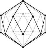
Figure 6. Two views of a spindle of girth $14$. The $3$-dimensional version, which looks like an antiprism capped off by two pyramids is the reason for the name.

Definition 6.2 (Spindles).

For some $k\geq 2$ let $(x_{1},x_{2},\ldots,x_{2k})$ be a sequence of $2k$ distinct elements in a bounded graded poset $P$ where the subscripts are viewed mod $2k$ and note that the parity of a subscript is well-defined in this context. Such a sequence forms a global spindle of girth $2k$ if for every $i$ with one parity, $x_{i-1}$ and $x_{i+1}$ are complements in $P_{\mathbf{0}x_{i}}$ and for every $i$ with the other parity, $x_{i-1}$ and $x_{i+1}$ are complements in $P_{x_{i}\mathbf{1}}$. See Figure 6. The elements $\mathbf{0}$ and $\mathbf{1}$ are called the endpoints of the global spindle and the sequence of elements $(x_{1},x_{2},\ldots,x_{2k})$ describes a zig-zag path in $P$ but with additional restrictions. There is also a local version. A (local) spindle, with or without the adjective, is a global spindle inside some interval $P_{zw}$ with endpoints $z$ and $w$.

Definition 6.3 (Short spindles).

The length of a global spindle is the length of the corresponding loop in the $1$-skeleton of the diagonal link of $P$ (endowed with the metric induced by the orthoscheme metric). A global spindle is short if its length is less than $2\pi$. The lengths of the individual edges in the diagonal link can be calculated using Proposition 4.8 and the reader should note that every edge in a diagonal link has length less than $\frac{\pi}{2}$. Thus every spindle of girth $4$ is short.

A spindle is a generalization of a bowtie in the following sense.

Proposition 6.4 (Spindles, bowties and lattices).

A bounded graded poset $P$ contains a bowtie iff it contains a spindle of girth $4$. In particular, $P$ is a lattice iff $P$ does not contains a spindle of girth $4$ and every bounded graded poset with no short spindles is a lattice.

Proof.

If $P$ contains a spindle of girth $4$ in the interval $P_{zw}$, then $x_{1}$, $x_{2}$, $x_{3}$ and $x_{4}$ form a bowtie since the bowtie conditions follow from the complementarity requirements. For example, $x_{2}$ is a maximal lower bound for $x_{1}$ and $x_{3}$ because $x_{1}$ and $x_{3}$ are complements in the interval $P_{x_{2}w}$. In the other direction suppose $a$, $b$, $c$, and $d$ form a bowtie, let $z$ be any maximal lower bound for $b$ and $d$ and let $w$ be any minimal upper bound for $a$ and $c$. It is then easy to check that $(a,b,c,d)$ is a global spindle of girth $4$ in the interval $P_{zw}$. The final assertion follows from Proposition 1.5 and the fact that every spindle of girth $4$ is short. ∎

The next step is to relate spindles and local geodesics in diagonal links. Let $P$ be a bounded graded poset and let $K$ be its orthoscheme complex. By Theorem 5.10 we know that determining whether or not $K$ is $\text{{CAT}}(0)$ reduces to determining whether or not an interval of $P$ has a diagonal link containing a short local geodesic. Since generic local geodesics are hard to describe and hard to detect, we shift our focus to the simplest local geodesics, i.e. those that remain in the $1$-skeleton of the local diagonal link. We now show that such paths are described by spindles. Figure 7 summarizes the relationships among these three classes of loops just described.

$\left\{\begin{array}[]{c}\textrm{Local geodesics}\\ \textrm{in a local}\\ \textrm{diagonal link}\end{array}\right\}$

$\supset$

$\left\{\begin{array}[]{c}\textrm{Local geodesics}\\ \textrm{that remain in}\\ \textrm{its $1$-skeleton}\end{array}\right\}$

$\subset$

$\left\{\begin{array}[]{c}\textrm{Loops that}\\ \textrm{correspond}\\ \textrm{to spindles}\end{array}\right\}$

Figure 7. The three types of loops discussed in this section.

Proposition 6.5 (Transitions and complements).

Let $P$ be a bounded graded poset and let $e_{xy}$ and $e_{yz}$ be distinct edges in the diagonal link of $P$. If the piecewise geodesic path from $v_{x}$ to $v_{y}$ to $v_{z}$ in the diagonal link of $P$ is locally geodesic at $v_{y}$ then either $x$ and $z$ are complements in the interval $P_{\mathbf{0}y}$ or $x$ and $z$ are complements in the interval $P_{y\mathbf{1}}$. As a consequence, every local geodesic loop in the diagonal link of $P$ that remains in its $1$-skeleton corresponds to a global spindle of $P$.

Proof.

First note that because the edges $e_{xy}$ and $e_{yz}$ exist, $x$ and $y$ are comparable in $P$ and $y$ and $z$ are comparable in $P$. If $x$ and $z$ are comparable as well then the path through $v_{y}$ is not locally geodesic because $x$, $y$ and $z$ form a chain, $v_{x}$, $v_{y}$ and $v_{z}$ are the corners of a convex spherical triangle in $\text{{lk}}(e_{\mathbf{0}\mathbf{1}},\lvert P\rvert)$ and the nonobtuse angle at $v_{y}$ (Corollary 4.9) shows that the path through $v_{y}$ is not locally geodesic because the transition vectors are not far apart. In the remaining cases both $x$ and $z$ are below $y$ or both $x$ and $z$ are above $y$. Assume that both are in $P_{\mathbf{0}y}$; the other case is analogous and omitted. If there is a $w$ in $P_{\mathbf{0}y}$ that is an upper bound of $x$ and $z$ other than $y$ or a lower bound of $x$ and $z$ other than $\mathbf{0}$ then there is a spherical triangle in $\text{{lk}}(e_{\mathbf{0}\mathbf{1}},\lvert P\rvert)$ with vertices $v_{w}$, $v_{y}$ and $v_{x}$ and a second triangle with vertices $v_{w}$, $v_{y}$ and $v_{z}$. As both triangles have acute angles at $v_{y}$ (Corollary 4.9) and the path through $v_{y}$ is not locally geodesic because the transition vectors are not far apart. For the final assertion suppose that $(x_{1},\ldots,x_{k})$ are the vertices of a local geodesic loop that remains in the $1$-skeleton of the diagonal link of $P$. The local result proved above means that adjacent triples satisfy the required conditions and it forces the orderings ($x_{i}<x_{i+1}$ or $x_{i}>x_{i+1}$) to alternate, making $k$ even. ∎

It is important to note that implication established above is in one direction only: a locally geodesic loop in the $1$-skeleton of a diagonal link must come from a spindle but not every spindle necessarily produces a locally geodesic loop. The problem is that just because $x$ and $z$ are complements in $P_{\mathbf{0}y}$ does not necessarily mean that $v_{x}$ and $v_{z}$ are far apart in $\text{{lk}}(v_{y},\lvert P\rvert)$ even though we conjecture that this is often the case.

Conjecture 6.6 (Complements are far apart).

Let $P$ be a bounded graded poset and let $K$ be its diagonal link. If $x$ and $y$ are complements in $P$ and $K$ is $\text{{CAT}}(1)$ then $v_{x}$ and $v_{y}$ are far apart in $K$.

We know that Conjecture 6.6 is true for the rank $n$ boolean lattice $P$ because the only elements that are complements in $P$ correspond to complementary subsets $A$ and $B$, these correspond to opposite corners of the $n$-cube $\lvert P\rvert$ and to antipodal points in the $n-1$ sphere that is the diagonal link of $P$. In particular, they represent points that are distance $\pi$ from each other in $\text{{lk}}(e_{\mathbf{0}\mathbf{1}},\lvert P\rvert)$. In fact, for boolean lattices, more is true.

Proposition 6.7 (Boolean spindles).

If $P$ is a boolean lattice of rank $n$ then every spindle in $P$ has girth $6$, length $2\pi$ and describes an equator of the $(n-1)$-sphere that is the diagonal link of $P$. In particular, $P$ has no short spindles.

Proof.

Let $(x_{1},x_{2},\ldots,x_{2k})$ be a spindle in $P$. Since intervals in boolean lattices are themselves boolean lattices, we may assume without loss of generality that this is a global spindle. Suppose $x_{1}<x_{2}$ and let $A$ and $B$ be the uniquely determined disjoint subsets of $[n]$ such that $x_{1}$ represents the set $A$ and $x_{2}$ represents the subset $A\cup B$. Finally let $C$ be the complement of $A\cup B$ in $[n]$. Since $x_{3}$ is a complement of $x_{1}$ in $P_{\mathbf{0}x_{2}}$ and complements in boolean lattices are unique, $x_{3}$ corresponds to the set $B$. Similarly, $x_{4}$ is a complement of $x_{2}$ in $P_{x_{3}\mathbf{1}}$ and thus must correspond to the set $B\cup C$. Continuing in this way, $x_{5}$, $x_{6}$, $x_{7}$ and $x_{8}$ correspond to the sets $C$, $A\cup C$, $A$ and $A\cup B$ respectively. Since the elements in a spindle are distinct, $x_{i}=x_{i+6}$ for all $i$ and the spindle has girth $6$. To see that its length $2\pi$, note that the fact that complements are far apart in boolean lattices means that global spindles describe paths that are embedded local geodesics in the diagonal link. In this case the diagonal link of $P$ is a sphere and the only embedded local geodesics are equatorial paths of length $2\pi$. ∎

We conclude this section by extending this result to modular lattices.

Definition 6.8 (Modular lattices).

A modular lattice is a graded lattice with the property that if $x$ and $y$ are complements in an interval $P_{zw}$ and $x$ has rank $i$ and corank $j$ in this interval, then $y$ has corank $i$ and rank $j$ in this interval. It should be clear from this definition that finite rank boolean lattices are examples of modular lattices as are the linear subspace posets described in Example 5.5.

Figure 8. A portion of a global spindle in a modular lattice that describes a local geodesic edge path of length $\pi$ in its diagonal link.

Proposition 6.9 (Modular spindles).

If $P$ is a bounded graded modular lattice then every spindle in $P$ has girth at least $6$ and describes a loop of length at least $2\pi$. In particular, $P$ has no short spindles.

Proof.

Since $P$ is a lattice, by Proposition 6.4 there are no spindles of length $4$. Thus every spindle has girth at least $6$. Next, since intervals in modular lattices are modular lattices we only need to consider global spindles. Let $(x_{1},x_{2},\ldots,x_{2k})$ be a global spindle with $x_{1}<x_{2}$ and let $i$, $j$ and $k$ be positive integers such that $x_{1}$ has rank $i$, $x_{2}$ has corank $k$ and $i+j+k=n$ where $n$ is the rank of $P$. The complementarity conditions and the definition of modularity imply that $x_{3}$ has rank $j$ and $x_{4}$ has corank $i$. See Figure 8. The key observation is that these are the same ranks and coranks and one of the geodesic paths between complementary subsets in a boolean lattice. In particular, the sum of the lengths of these edges in the diagonal link of $P$ is exactly $\pi$. Since the girth of the spindle is at least $6$, its length is at least $2\pi$. This completes the proof. ∎

Since bounded graded modular lattices have no short spindles, the poset curvature conjecture leads us to conjecture the following.

Conjecture 6.10 (Modular lattices and $\text{{CAT}}(0)$).

Every bounded graded modular lattice has a $\text{{CAT}}(0)$ orthoscheme complex.

7. Low rank

In this section we shift our attention from bounded posets of arbitrary rank to those of rank at most $4$. Our goal is to prove the poset curvature conjecture in this context, thus establishing Theorem A. The proof depends on two basic results. The first is that complementary elements in a low rank poset correspond to vertices that are always far apart in its diagonal link.

Lemma 7.1 (Low rank complements).

If $x$ and $y$ are complements in a poset $P$ of rank at most $3$ then $v_{x}$ and $v_{y}$ are far apart in its diagonal link.

Proof.

If $P$ has rank less than $3$ then its diagonal link has no edges and $v_{x}$ and $v_{y}$ are trivially far apart. Thus we may assume that the rank of $P$ is $3$. In this case, the diagonal link is a bipartite metric graph where every edge has length $\frac{\pi}{3}$ and connects an element of rank $1$ to an element of rank $2$. As a consequence $v_{x}$ and $v_{y}$ are not far apart iff their combinatorial distance is less than $3$. Distance $1$ means $x<y$ or $x>y$ and distance $2$ means $x$ and $y$ are both rank $1$ with a common rank $2$ upper bound or both rank $2$ with a common rank $1$ lower bound. All of these situations are excluded by the hypothesis that $x$ and $y$ are complements. ∎

This result has consequences for piecewise geodesic paths in the $1$-skeleton of the diagonal link.

Lemma 7.2 (Low rank transitions).

Let $P$ be a bounded graded poset of rank at most $4$. If $x$, $y$ and $z$ are distinct elements of $P$ such that $x$ and $z$ are complements in $P_{\mathbf{0}y}$ or complements in $P_{y\mathbf{1}}$, then the edge path from $v_{x}$ to $v_{y}$ to $v_{z}$ in the diagonal link of $P$ is locally geodesic.

Proof.

Suppose $x$ and $z$ are complements in $P_{\mathbf{0}y}$; the other case is analogous. By Lemma 7.1 $v_{x}$ and $v_{z}$ are far apart in $\text{{lk}}(e_{\mathbf{0}y},\lvert P_{\mathbf{0}y}\rvert)$ since $P_{\mathbf{0}y}$ is a poset of rank at most $3$. Recall that the link of $v_{y}$ in the diagonal link of $P$ is the spherical join $\text{{lk}}(e_{\mathbf{0}y},\lvert P_{\mathbf{0}y}\rvert)\ast\text{{lk}}(e_{y\mathbf{1}},\lvert P_{y\mathbf{1}}\rvert)$. The fact that $v_{x}$ and $v_{z}$ are far apart in one factor means that $v_{x}$ and $v_{z}$ are far apart in the spherical join. As a consequence, the path from $v_{x}$ to $v_{y}$ to $v_{z}$ in the diagonal link of $P$ is locally geodesic. ∎

Lemma 7.2 quickly implies one-half of Theorem A.

Theorem 7.3 (Low rank spindles).

If $P$ is a bounded graded poset of rank at most $4$, then global spindles in $P$ describe local geodesic loops in its diagonal link. As a consequence, if $P$ contains a short spindle, global or local, then the orthoscheme complex of $P$ is not $\text{{CAT}}(0)$.

Proof.

The first assertion follows immediately from Lemma 7.2. To see the second, suppose $P$ contains a short spindle and restrict to the interval where it is global. Since the spindle describes a short local geodesic loop in this local diagonal link, it is not $\text{{CAT}}(1)$ and by Theorem 5.10 the orthoscheme complex of $P$ is not $\text{{CAT}}(0)$. ∎

Having established that the existence of short spindles in low rank posets prevent its orthoscheme complex from being $\text{{CAT}}(0)$, we pause for a moment to clarify exactly which spindles in low rank posets are short. First note that every spindle of girth $4$ is short (since edges in the diagonal link have length less than $\frac{\pi}{2}$) and they occur iff the poset is not a lattice (Proposition 6.4). Thus we only need to consider spindles in lattices.

Proposition 7.4 (Short spindles).

If a bounded graded lattice $P$ of rank at most $4$ contains a short spindle, then $P$ has rank $4$, the spindle is a global spindle of girth $6$ and its elements alternate between two adjacent ranks.

Proof.

After replacing $P$ by one its intervals if necessary we may assume that the spindle under consideration is a global spindle in $P$ and, since $P$ is a lattice, it must have girth at least $6$. If $P$ has rank $3$ (lower ranks are too small to contain spindles) then all edges in the diagonal link of $P$ have length $\frac{\pi}{3}$ and the spindle is not short. Thus $P$ has rank $4$. In rank $4$ there are two possible edge lengths: the shorter edges connect adjacent ranks and have length $\arccos\left(\sqrt{\frac{1}{3}}\right)\cong.304\pi$ and the longer edges connect ranks $1$ and $3$ and have length $\arccos\left(\frac{1}{3}\right)\cong.392\pi$. (Exact values are calculated using Proposition 4.8.) Since both lengths are more than $\frac{\pi}{4}$, spindles of girth $8$ or more are not short. Finally, since one long and two short edges have total length exactly $\pi$ and spindles in this setting have to have an even number of longer edges, the only short spindles are those involving six short edges creating a zig-zag path between two adjacent ranks as shown in Figure 9. ∎

Figure 9. Short spindles in rank $4$ lattices.

We should note that these low rank short spindles are closely related to the empty triangles that arise when testing the curvature of cube complexes. Bowties cannot occur in the face poset of a cube complex and the empty triangles that prevent cube complexes from being $\text{{CAT}}(0)$ correspond to one of the short spindles of girth $6$ just described.

Remark 7.5 (Short spindles and empty triangles).

Let $K$ be cube complex that is not $\text{{CAT}}(0)$ and let $\sigma$ be a cell in $K$ whose link contains an empty triangle (Proposition 3.4). The zig-zag path shown on the lefthand side of Figure 9 corresponds to a portion of the face poset of the link of $\sigma$ in $K$. The three elements in rank $1$ and the three elements in rank $2$ correspond to the three vertices and edges respectively of a triangle in the link of $\sigma$ and the absence of an element of rank $3$ which caps off this zig-zag path corresponds to the fact that the triangle is empty.

We now return to the proof of Theorem A. The second basic result we need is that whenever the diagonal link of a low rank poset contains a short local geodesic, that local geodesic can be homotoped into the $1$-skeleton of the diagonal link without increasing its length. For posets of rank strictly less than $4$ there is nothing to prove and for rank $4$ posets we appeal to earlier work by Murray Elder and the second author [9]. The key concept we need is that of a gallery.

Definition 7.6 (Galleries).

Given a local geodesic loop $\gamma$ in a PS complex $K$ one can construct a new PS complex $L$ called a gallery such that the map $\gamma$ from a metric circle to $K$ factors through an embedding of the circle into $L$ and a cellular immersion of $L$ into $K$. The rough idea is to glue together copies of the cells through which $\gamma$ passes in $K$. More specifically, every point in the path $\gamma$ is contained in a uniquely defined open simplex. For this well-defined linear or cyclic sequence of open simplices, take a copy of the corresponding closed simplices and glue them together in the minimal way possible so that the result is a PS complex that maps to $K$ and the curve $\gamma$ lifts though this map. See [9] for additional detail.

Definition 7.7 (Types of galleries).

So long as the lengths of edges in $K$ are less than $\frac{\pi}{2}$, the gallery $L$ will be homotopy equivalent to a circle and the image of the circle in $L$ will have winding number $1$. Moreover, if $K$ is $2$-dimensional and the loop $\gamma$ does not pass through a vertex of $K$ then $L$ will be a $2$-manifold with boundary called either an annular gallery or a möbius gallery depending on its topology. If $\gamma$ does pass through a vertex of $K$ then $L$ is called a necklace gallery and it can be broken up into segments called beads corresponding to a portion of $\gamma$ starting at a vertex, ending at a vertex and not passing through a vertex in between.

In [9] a computer program was used to systematically enumerate the finite list of possible galleries determined by a short local geodesic in the vertex link of a PE complex built out of $\widetilde{A}_{3}$ Coxeter shapes. (An $\widetilde{A}_{n}$ Coxeter shape is a PE tetrahedron whose vertex links are Coxeter shapes of type $A_{n}$. One general definition of these shapes is given in Definition 8.2.) The results of this enumeration are listed in Figures 10, 11, and 12 according to the following conventions. The triangles shown should be viewed as representing spherical triangles: the angles that look like $\pi/2$ angles are in fact $\pi/2$ angles, while the $\pi/4$ angles are meant to represent $\pi/3$ angles. Thus, in the third figure of Figure 12 both sides connecting the specified end cells are actually geodesics as can be seen in a more suggestive representation of the same configuration shown on the righthand side of Figure 13. The heavily shaded leftmost and rightmost edges in the configurations shown in Figure 10 should be identified to produce annuli and the heavily shaded leftmost and rightmost edges in the configurations shown in Figure 11 should be identified with a half-twist to produce möbius strips. The three configurations shown in Figure 12 are three of the beads from which necklace galleries are formed. They are labeled $C$, $D$ and $E$ since $A$ and $B$ are used to denote the short and long edges, respectively, thought of as beads. The following result was proved in [9].

Figure 10. Two annular galleries.

Figure 11. Four möbius galleries.

$C$	$D$	$E$

Figure 12. Three non-trivial beads.

Proposition 7.8 (Short $A_{3}$ geodesics).

Let $K$ be a vertex link of a PE complex built out of $\widetilde{A}_{3}$ Coxeter shapes. If this PS complex built out of $A_{3}$ Coxeter shapes is not quite $\text{{CAT}}(1)$ then it contains a short local geodesic loop $\gamma$ that determines a gallery $L$ that is either one of the two annular galleries listed in Figure 10, one of the four möbius galleries listed in Figure 11, or a necklace gallery formed by stringing together the short edge $A$, the long edge $B$, and the three nontrivial beads shown in Figure 12 in one of $26$ particular ways. In particular, the $26$ necklace galleries that contain a short geodesic loop are described by the following sequences of beads: $A^{2}$, $A^{4}$, $A^{6}$, $A^{2}B$, $A^{2}B^{2}$, $A^{2}B^{3}$, $ABAC$, $A^{2}C$, $A^{2}C^{2}$, $A^{2}D$, $A^{2}E$, $A^{4}B$, $CA^{4}$, $B$, $B^{2}$, $B^{3}$, $B^{4}$, $B^{5}$, $BE$, $B^{2}E$, $C$, $C^{2}$, $C^{3}$, $CD$, $D$, and $E$.

The relevence of Proposition 7.8 in the current setting is that the diagonal link of a bounded graded rank $4$ poset is a complex built out of $A_{3}$ spherical simplices in a way that could have arisen as a vertex link of a PE complex built out of $\widetilde{A}_{3}$ shapes. We will comment more on this connection in §8. In particular, if the diagonal link of a bounded graded rank $4$ poset is not quite $\text{{CAT}}(1)$ then it contains a short unshrinkable local geodesic loop that determines one of the $32$ specific galleries listed above.

Lemma 7.9 (Loops and vertices).

Let $K$ be the diagonal link of a bounded graded rank $4$ poset $P$. If $K$ is not quite $\text{{CAT}}(1)$ and $\gamma$ is a short unshrinkable locally geodesic loop in $K$, then $\gamma$ passes through a vertex of $K$.

Proof.

Let $L$ be the gallery associated to $\gamma$. If $L$ is an annular gallery then $\gamma$ is shrinkable via the analog of homotoping an equator through lines of latitude, contradicting our hypothesis. If $L$ is a möbius gallery, then it is one of the four listed in Figure 11. Since $L$ immerses into the order complex $K$ of the diagonal link of a rank $4$ poset we should be able to label each vertex of $L$ by the rank of the element of $P$ that corresponds to its image in $K$. In particular, the three vertices of a triangle should receive three distinct numbers from the list $\{1,2,3\}$. Once one triangle in $L$ is labeled, the remaining labels are forced and in each instance, the möbius strip cannot be consistently labelled. As a result $L$ cannot be a möbius gallery. The only remaining possibility is that $L$ is a necklace gallery and $\gamma$ passes through a vertex of $K$. ∎

Figure 13. A poset configuration and the corresponding PS configuration.

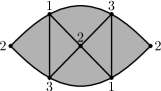
Figure 14. A poset configuration and the corresponding PS configuration.

Theorem 7.10 (Restricting to the $1$-skeleton).

Let $P$ be a bounded graded poset of rank at most $4$. If a local diagonal link of $P$ is not quite $\text{{CAT}}(1)$ then it contains a short local geodesic loop that remains in its $1$-skeleton. In particular, when the orthoscheme complex of $P$ is not $\text{{CAT}}(0)$, $P$ contains a short spindle.

Proof.

Since the diagonal link of an interval is $1$-dimensional when $P$ has rank less than $4$, the first assertion is trivial in that case. Thus assume that $P$ has rank $4$ and that we are considering the diagonal link $K=\text{{lk}}(e_{\mathbf{0}\mathbf{1}},\lvert P\rvert)$. Because $K$ is not quite $\text{{CAT}}(1)$, it is locally $\text{{CAT}}(1)$ but contains a short locally geodesic loop $\gamma$. By Lemma 3.6 and Lemma 7.9 we may also assume that $\gamma$ is both unshrinkable and that it is associated with a necklace gallery $L$. The necklace $L$ is a string of beads of type $A$, $B$, $C$, $D$ and $E$. The bead of type $E$ is a lune, the portion of the geodesic it contains is of length $\pi$, and there is a length-preserving endpoint-preserving homotopy that moves this portion of $\gamma$ into the boundary of $E$. This has the effect of replacing $E$ with a sequence of edges ($AAB$ or $BAA$). See Figure 13. Similarly, if $L$ contains a bead of type $D$, then $P$ contains a configuration that produces the lune shown in Figure 14. The portion of the geodesic it contains is of length $\pi$, and there is a length-preserving endpoint-preserving homotopy that moves this portion of $\gamma$ into the boundary of the lune. This has the effect of replacing $D$ with a sequence of edges $ABA$. Thus we may assume that $L$ contains no beads of type $D$ or $E$.

Finally, suppose $L$ contains a bead of type $C$ and consider the bead immediately after it. It cannot be of type $B$ since $C$ ends at a vertex of rank $2$ so it is either type $A$ or another bead of type $C$. If type $A$ then we have all but one element of the configuration shown on the lefthand side of Figure 13 and there is an additional triangle in $K$ that gives us a way to shorten $\gamma$, contradicting its unshrinkability. On the other hand, if the next bead has type $C$ (and there are no obivous shortenings) then we have the configuration shown on the lefthand side of Figure 14. Thus there are triangles present in $K$ that enable us to perform a length-preserving endpoint preserving homotopy of this portion of $\gamma$ through beads of type $CC$ to a path in the $1$-skeleton passing through edges of type $ABA$. In short, whenever $\gamma$ leaves the $1$-skeleton, there is a way to locally modify the path so that its length never increases and the new path passes through fewer $2$-cells. Iterating this process proves the first assertion and the second assertion follows from Proposition 6.5. ∎

Combining Theorem 7.3 and Theorem 7.10 establishes the following.

Theorem A.

The orthoscheme complex of a bounded graded poset $P$ of rank at most $4$ is $\text{{CAT}}(0)$ iff $P$ is a lattice with no short spindles.

As a quick application note that Theorem A implies that every modular poset of rank at most $4$ has a $\text{{CAT}}(0)$ orthoscheme complex with a $\text{{CAT}}(1)$ diagonal link. In particular, the theorem shows that the linear subspace poset $L_{4}(\mathbb{F})$ has a $\text{{CAT}}(0)$ orthoscheme complex for every field $\mathbb{F}$ and its diagonal link, which is a thick spherical building of type $A_{3}$, is $\text{{CAT}}(1)$. That the link is $\text{{CAT}}(1)$ is well-known. See, for example, [1] or [10].

8. Artin groups

In this final section we first apply Theorem A to a poset closely associated with the $5$-string braid group and then, at the end of the section, we extend the discussion to the other four generator Artin groups of finite-type. For the braid group, the relevant poset is the lattice of noncrossing partitions.

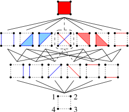
Figure 15. The figure shows the partition lattice $\Pi_{4}$ with the blocks indicated by their convex hulls. If the portion surrounded by a dashed line is removed, the result is the noncrossing partition lattice $NC_{4}$.

Definition 8.1 (Partitions and noncrossing partitions).

Recall that a partition of a set is a pairwise disjoint collection of subsets (called blocks) whose union is the entire set. These partitions are naturally ordered by refinement, i.e. one partition is less than another is each block of the first is contained in some block of the second. The resulting bounded graded lattice is called the partition lattice. Its maximal element has only one block, its minimal element has singleton blocks and the rank of an element is determined by the number of blocks it contains. When the underlying set is $[n]=\{1,2,\ldots,n\}$ the partition lattice is denoted $\Pi_{n}$ and it has rank $n-1$. The rank $3$ poset $\Pi_{4}$ is shown in Figure 15. A noncrossing partition is a partition of the vertices of a regular $n$-gon (consecutively labeled by the set $[n]$) so that the convex hulls of its blocks are pairwise disjoint. Figure 16 shows the noncrossing partition $\{\{1,4,5\},\{2,3\},\{6,8\},\{7\}\}$. A partition such as $\{\{1,4,6\},\{2,3\},\{5,8\},\{7\}\}$ would be crossing. For $n=4$, the only difference between $\Pi_{4}$ and $NC_{4}$ is the partition $\{\{1,3\},\{2,4\}\}$ which is not noncrossing. The subposet of noncrossing partitions is also a bounded graded rank $n$ lattice. In addition, $NC_{n}$ is self-dual in the sense that there exists an order-reversing bijection from $NC_{n}$ to itself ([4],[11]).

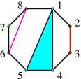
Figure 16. A noncrossing partition of the set $[8]$.

The close connection between the braid groups and the noncrossing partition lattice can briefly be described as follows. There is a way of pairwise identifying faces of the orthoscheme complex of $NC_{n}$ by isometries so that the result is a one-vertex complex $X$ with a contractible universal cover and the $n$-string braid group as its fundamental group. See [4] for details. Moreover, under the orthoscheme metric, the metric space $X$ metrically splits as a direct product of a compact PE complex $Y$ and a circle of length $\sqrt{n}$. We should note, however, that this split is not visible in the cell structure of $X$. The splitting into a direct product is easiest to see in the universal cover $\widetilde{X}\cong\widetilde{Y}\times\mathbb{R}$ where the standard $n$-orthoschemes naturally fit together into columns.

Definition 8.2 (Columns).

Fix $n\in\mathbb{N}$ and consider the following collection of points in $\mathbb{R}^{n}$. For each integer $m$ write $m=qn+r$ where $q$ and $r$ are the unique integers with $0\leq r<n$ and let $v_{m}$ denote the point $((q+1)^{r},q^{n-r})\in\mathbb{R}^{n}$ using the same shorthand notation as in the proof of Proposition 4.8. To illustrate, when $m=-22$ and $n=8$ then $q=-3$, $r=2$ and $v_{-22}=(-2^{2},-3^{6})$. Note that the vector from $v_{m}$ to $v_{m+1}$ is a unit basis vector and that the particular unit basis vector is specified by the value of $r$. In particular, any $n+1$ consecutive vertices of the bi-infinite sequence $(\ldots v_{-2},v_{-1},v_{0},v_{1},v_{2}\ldots)$ are the vertices of a standard $n$-orthoscheme. It is easy to check that the standard $n$-orthoscheme $\textsf{Ortho}(v_{0},v_{1},\ldots,v_{n})$ is defined by the inequalities $1\geq x_{1}\geq x_{2}\geq\cdots\geq x_{n}\geq 0$ and that the union of the orthoschemes defined by $n+1$ consecutive vertices of this sequence is a convex shape defined by the inequalities $x_{1}\geq x_{2}\geq\cdots\geq x_{n}\geq x_{1}-1$. We call this configuration of orthoschemes a column. Because these equalities are invariant under the addition of multiples of the vector $(1^{n})$, the result is metrically a direct product of a $(n-1)$-dimensional shape with the real line. It turns out that the cross-section perpendicular to the direction $(1^{n})$ is a Euclidean polytope known as the Coxeter simplex of type $\widetilde{A}_{n-1}$ and that every vertex of this polytope has a link isometric to the diagonal link of the standard $n$-orthoscheme, namely, the convex spherical polytope of type $A_{n-1}$ that we called $\alpha_{n-1}$. To illustrate, when $n=3$ the column just defined is a direct product of an $\widetilde{A}_{2}$ Euclidean polytope with $\mathbb{R}$ and the diagonal link of a $3$-orthoscheme is the spherical polytope of type $A_{2}$. In this case the PE shape $\widetilde{A}_{2}$ is an equilateral triangle and the PS shape $A_{2}$ is an arc of length $\frac{\pi}{3}$.

Returning to the Eilenberg-MacLane space for the $n$-string braid group, recall that a group is called a $\text{{CAT}}(0)$ group if it acts properly discontinuously cocompactly by isometries on a complete $\text{{CAT}}(0)$ space. For our purposes, the only fact we need is that the fundamental group of any compact locally $\text{{CAT}}(0)$ PE complex is a $\text{{CAT}}(0)$ group since its action on the universal cover by deck transformations has all of the necessary properties. If $X$ is the Eilenberg-MacLane space for the $n$-string braid group built from the orthoscheme complex of the noncrossing partition lattice $NC_{n}$, then as a metric space $X$ is a direct product of a circle of length $\sqrt{n}$ and a PE complex $Y$ built out of $\widetilde{A}_{n-1}$ shapes. Moreover, the link of the unique vertex in $Y$ is isometric to the diagonal link of $NC_{n}$. As a consequence, if the orthoscheme complex of the noncrossing partition lattice $NC_{n}$ is $\text{{CAT}}(0)$, then $Y$ is locally $\text{{CAT}}(0)$, $X$ is locally $\text{{CAT}}(0)$ and the $n$-string braid group is a $\text{{CAT}}(0)$ group. In short we have the following implication.

Proposition 8.3 (Partitions and braids).

If the orthoscheme complex of the noncrossing partition lattice $NC_{n}$ is $\text{{CAT}}(0)$, then the $n$-string braid group is a $\text{{CAT}}(0)$ group.

Since we (firmly) believe that the orthoscheme complex of $NC_{n}$ is indeed $\text{{CAT}}(0)$ for every $n$, we formalize this assertion as a conjecture.

Conjecture 8.4 (Curvature of $NC_{n}$).

For every $n$, the orthoscheme complex of the noncrossing partition lattice $NC_{n}$ is $\text{{CAT}}(0)$ and as a consequence, the braid groups are $\text{{CAT}}(0)$ groups.

One reason we believe that Conjecture 8.4 is true has to do with the close connection between noncrossing partitions, partitions and linear subspaces.

Remark 8.5 (Partitions and linear subspaces).

If $\mathbb{F}$ is a field and $\mathbb{F}^{n}$ is a vector space with a fixed coordinate system then there is a natural injective map from $\Pi_{n}$ to $L_{n}(\mathbb{F})$ that sends each partition to the subspace of vectors where the sum of the coordinates whose indices all belong to the same block sum to $0$. For example, the partition $\{\{1,3,4\},\{2,5\},\{6\},\{7\}\}$ is sent to the $3$-dimensional subspace of $\mathbb{F}^{7}$ satisfying the equations $x_{1}+x_{3}+x_{4}=0$, $x_{2}+x_{5}=0$, $x_{6}=0$, and $x_{7}=0$. The partition with one singleton blocks is sent to the $0$-dimensional subspace and the partition with one block is sent to the $(n-1)$-dimensional subspace where all coordinates sum to $0$. Thus the map from $\Pi_{n}$ to $L_{n}(\mathbb{F})$ can be restricted to a map from $\Pi_{n}$ to $L_{n-1}(\mathbb{F})$ but at the cost of being harder to describe. The relationship between the noncrossing partition lattice, the partition lattice and the lattice of linear subspaces is therefore $NC_{n}\subset\Pi_{n}\hookrightarrow L_{n-1}(\mathbb{F})$.

As we remarked earlier, the diagonal link of $L_{n-1}(\mathbb{F})$ is a $\text{{CAT}}(1)$ complex known as a thick spherical building. Thus, the inclusion just established means that the diagonal link of $NC_{n}$ is a subcomplex of a thick spherical building. For those familiar with the structure of buildings, we note that a much stronger statement is true.

Proposition 8.6 (Partitions and apartments).

Every chain in $NC_{n}$ belongs to a boolean subposet. As a consequence, for every field $\mathbb{F}$, the diagonal link of $NC_{n}$ is a union of apartments in the thick spherical building constructed as the diagonal link of $L_{n-1}(\mathbb{F})$.

Proof sketch.

Since Proposition 8.6 is not needed below, we shall not give a complete proof, but the rough idea goes as follows. Every chain of noncrossing paritions can be extended to a maximal chain, and given any maximal chain, it is possible to systematically extract a planar spanning tree of the regular $n$-gon with edges labeled $1$ through $n-1$ such that the connected components of the graph containing only edges $1$ through $i$ are the blocks of the rank $i$ noncrossing partition in the chain. Once such a labeled spanning tree has been found, the noncrossing partitions that arise from the connected components of the graph with an arbitrary subset of these edges form a boolean subposet of $NC_{n}$. The second assertion follows since boolean subposets give rise to spheres in the diagonal link that are the apartments of the spherical building. ∎

The fact that the diagonal link of $NC_{n}$ is a union of apartments inside a thick spherical building is circumstantial evidence that the diagonal link is $\text{{CAT}}(1)$, the orthoscheme complex of $NC_{n}$ is $\text{{CAT}}(0)$ and that the corresponding Eilenberg-MacLane space for the $n$-string braid group is $\text{{CAT}}(0)$. By Theorem A, these conjectures are true for $n=5$.

Proposition 8.7 (Curvature of $NC_{5}$).

The orthoscheme complex of $NC_{5}$ is $\text{{CAT}}(0)$ and, as a consequence, the $5$-string braid group is a $\text{{CAT}}(0)$ group.

Proof.

Since the rank $4$ poset $NC_{5}$ is known to be a lattice, by Theorem A and Proposition 7.4 we only need to check that $NC_{5}$ does not contain a global spindle of girth $6$ whose elements alternate between adjacent ranks. Moreover, because $NC_{5}$ is self-dual, it is sufficient to rule out the configuration on the lefthand side of Figure 9. Finally, if there were such a configuration, the three rank $1$ elements would correspond to noncrossing parititions each containing a single edge and the fact that they pairwise have rank $2$ joins indicates that these edges are pairwise noncrossing. But under these conditions, the join of all three elements will have rank $3$ contrary to the desired configuration. Thus $NC_{5}$ has no short spindles, its orthoscheme complex is $\text{{CAT}}(0)$ and the $5$-string braid group is a $\text{{CAT}}(0)$ group. ∎

We should note that we originally proved that the $5$-string braid group is a $\text{{CAT}}(0)$ group in a more direct fashion (unpublished) shortly after the first author introduced his new Eilenberg-MacLane spaces for the braid groups [4], a direct computation carried out independently and contemporaneously by Daan Krammer (also unpublished). And finally, we indicate how the above analysis of the $5$-string braid group can be extended to cover the other four-generator Artin groups of finite-type. The posets and complexes defined via the symmetric group in [4] were extended to the other finite Coxeter groups in [5]. The first author’s work with Colum Watt produces bounded graded lattices with a uniform definition that can be used to construct Eilenberg-MacLane spaces for groups called Artin groups of finite-type. We begin by roughly describing these additional posets.

Definition 8.8 ($W$-noncrossing partitions).

Let $W$ be a finite Coxeter group with standard minimal generating set $S$ and let $T$ be the closure of $S$ under conjugacy. The set $S$ is called a simple system and $T$ is the set of all reflections. A Coxeter element in $W$ is an element $\delta$ that is a product of the elements in $S$ in some order. For the finite Coxeter groups, the order chosen is irrelevant since the result is well-defined up to conjugacy. The poset of $W$-noncrossing partitions $NC_{W}$ is the derived from the minimum length factorizations of $\delta$ into elements of $T$ or equivalently, it represents an interval in the Cayley graph of $W$ with respect to $T$ that starts at the identity and ends at $\delta$. The name alludes to the fact that when $W$ is the symmetric group $\textsf{Sym}_{n}$, a Coxeter element is an $n$-cycle and the poset $NC_{W}$ is isomorphic to the lattice of noncrossing partitions previously defined.

For each finite Coxeter group $W$, the poset $NC_{W}$ is a finite bounded graded lattice whose rank $n$ is the size of the standard minimal generating set $S$ for $W$. As was the case with the braid groups, there is a one-vertex complex $X$ constructed by identifying faces of the orthoscheme complex of $NC_{W}$. This complex splits as a metric direct product of a complex $Y$ constructed from $\widetilde{A}_{n-1}$ shapes and a circle of length $\sqrt{n}$, and the universal cover $\widetilde{X}$ decomposes into columns as before. In particular, $\widetilde{X}$ is isometric with $\widetilde{Y}\times\mathbb{R}$, the link of the unique vertex of $Y$ is isometric to the diagonal link of the orthoscheme complex of $NC_{W}$, and we have the following result that generalizes Proposition 8.3.

Proposition 8.9 (Partitions and Artin groups).

Let $W$ be a finite Coxter group and let $NC_{W}$ be its lattice of noncrossing partitions. If the orthoscheme complex of $NC_{W}$ is $\text{{CAT}}(0)$ then the finite-type Artin group corresponding to $W$ is a $\text{{CAT}}(0)$ group.

When $W$ has a standard minimal generating set of size $4$, the poset $NC_{W}$ has rank $4$ and Theorem A can be applied as above. Each of the five possible posets (corresponding to the finite Coxeter groups of type $A_{4}$, $B_{4}$, $D_{4}$, $F_{4}$ and $H_{4}$) is known to be a lattice and thus by Proposition 7.4 we only need to check whether or not $NC_{W}$ contain a global spindle of girth $6$ whose elements alternate between adjacent ranks. Moreover, because $NC_{W}$ is self-dual ([11]), it is sufficient to search for the configuration on the lefthand side of Figure 9. The second author wrote a short program in GAP to construct these posets and to search for this particular configuration. The noncrossing posets of type $A_{4}$ and $B_{4}$ contain no such configurations but the noncrossing posets of type $D_{4}$, $F_{4}$ and $H_{4}$ do contain such configurations. By Theorem A and Proposition 8.9, this establishes the following.

Theorem B (Artin groups).

Let $K$ be the Eilenberg-MacLane space for a four-generator Artin group of finite type built from the corresponding poset of $W$-noncrossing partitions and endowed with the orthoscheme metric. When the group is of type $A_{4}$ or $B_{4}$, the complex $K$ is $\text{{CAT}}(0)$ and the group is a $\text{{CAT}}(0)$ group. When the group is of type $D_{4}$, $F_{4}$ or $H_{4}$, the complex $K$ is not $\text{{CAT}}(0)$.

References

- [1] Peter Abramenko and Kenneth S. Brown. Buildings, volume 248 of Graduate Texts in Mathematics. Springer, New York, 2008. Theory and applications.
- [2] A. Björner. Topological methods. In Handbook of combinatorics, Vol. 1, 2, pages 1819–1872. Elsevier, Amsterdam, 1995.
- [3] B. H. Bowditch. Notes on locally spaces. In Geometric group theory (Columbus, OH, 1992), pages 1–48. de Gruyter, Berlin, 1995.
- [4] Thomas Brady. A partial order on the symmetric group and new ’s for the braid groups. Adv. Math., 161(1):20–40, 2001.
- [5] Thomas Brady and Colum Watt. ’s for Artin groups of finite type. In Proceedings of the Conference on Geometric and Combinatorial Group Theory, Part I (Haifa, 2000), volume 94, pages 225–250, 2002.
- [6] Martin R. Bridson. Geodesics and curvature in metric simplicial complexes. In Group theory from a geometrical viewpoint (Trieste, 1990), pages 373–463. World Sci. Publishing, River Edge, NJ, 1991.
- [7] Martin R. Bridson and André Haefliger. Metric spaces of non-positive curvature, volume 319 of Grundlehren der Mathematischen Wissenschaften [Fundamental Principles of Mathematical Sciences]. Springer-Verlag, Berlin, 1999.
- [8] H. S. M. Coxeter. Regular complex polytopes. Cambridge University Press, Cambridge, second edition, 1991.
- [9] Murray Elder and Jon McCammond. Curvature testing in 3-dimensional metric polyhedral complexes. Experiment. Math., 11(1):143–158, 2002.
- [10] A. Lytchak. Rigidity of spherical buildings and joins. Geom. Funct. Anal., 15(3):720–752, 2005.
- [11] Jon McCammond. Noncrossing partitions in surprising locations. Amer. Math. Monthly, 113(7):598–610, 2006.
- [12] Richard P. Stanley. Enumerative combinatorics. Vol. 1, volume 49 of Cambridge Studies in Advanced Mathematics. Cambridge University Press, Cambridge, 1997. With a foreword by Gian-Carlo Rota, Corrected reprint of the 1986 original.
- [13] Günter M. Ziegler. Lectures on polytopes, volume 152 of Graduate Texts in Mathematics. Springer-Verlag, New York, 1995.