Temporal variations of the CaXIX spectra in solar flares

Abstract

Aims. Standard model of solar flares comprises a bulk expansion and rise of abruptly heated plasma (the chromospheric evaporation). Emission from plasma ascending along loops rooted on the visible solar disk should be often dominated, at least temporally, by a blue-shifted emission. However, there is only a very limited number of published observations of solar flares having spectra in which the blue-shifted component dominates the stationary one. In this work we compare observed X-ray spectra of three solar flares recorded during their impulsive phases and relevant synthetic spectra calculated using one-dimensional hydro-dynamic numerical model of these flares. The main aim of the work was to explain why numerous flares do not show blue-shifted spectra.

Methods. We synthetised time series of BCS spectra of three solar flares in various moments of their evolution from the beginning of the impulsive phases beyond maxima of the X-ray emissions using 1D numerical model of the solar flares and standard software to calculate BCS synthetic spectra of the flaring plasma. The models of the flares were calculated using observed energy distributions of the non-thermal electron beams injected into the loops, initial values of the main physical parameters of the plasma confined in the loops and geometrical properties loops’ estimated using available observational data. The synthesized BCS spectra of the flares were compared with the relevant observed BCS spectra.

Results. Taking into account the geometrical dependences of the line-of-sight velocities of the plasma moving along the flaring loop inclined toward the solar surface as well as a distribution of the investigated flares over the solar disk, we conclude that stationary component of the spectrum should be observed almost for all flares during their early phases of evolution. In opposite, the blue-shifted component of the spectrum could be not detected in flares having plasma rising along the flaring loop even with high velocity due to the geometrical dependences only. Our simulations based on realistic heating rates of plasma by non-thermal electrons indicate also that the upper chromosphere is heated by non-thermal electrons a few seconds before beginning of noticeable high-velocity bulk motions, and before this time plasma emits stationary component of the spectrum only. After the start of the up-flow motion, the blue-shifted component dominate temporally the synthetic spectra of the investigated flares at their early phases.

1 Introduction

Solar flares are powered mainly by high-energy non-thermal electrons accelerated somewhere in the solar corona which stream along magnetic field lines toward the chromosphere and even photosphere and deposit there its energy mostly in Coulomb collisions. However, a small fraction of the energy carried by non-thermal electrons is converted into hard X-rays (HXR) by bremsstrahlung processes (Brown (1973)). Rapid deposition of energy by the electron beams cause that the energy cannot be radiated away sufficiently fast, therefore a strong pressure imbalanced develops, and heated plasma expands up into corona in a process known as chromospheric evaporation (Antonucci et al., 1984; Fisher, 1985; Antonucci et al., 1999).

The heated and evaporates plasma radiates over a wide spectral range from hard X-rays or even gamma rays to radio emission, but most of the energy is emitted in soft X-rays (SXR) (Lin & Hudson, 1971; Petrosian, 1973). Hard and soft X-ray fluxes emitted by solar flares are generally related, in a way first described by Neupert (1968), who found that the time derivative of the soft X-ray flux approximately matches the microwave flux during the flare impulsive burst. A similar effect was also observed for hard X-ray emission (Dennis & Zarro (1993)). Since hard X-ray and microwave emissions is produced by non-thermal electrons and soft X-rays are generated by thermal emission from hot plasma, the Neupert effect suggests that non-thermal electrons are primary source of plasma heating.

Detailed studies (Dennis & Zarro, 1993; Veronig et al., 2002) show deviations from the Neupert effect, indicating that involved processes are much more complicated. There are clear evidence of a SXR rise before the impulsive HXR emission in some flares (often referred to as a preheating), a persistence of the increase and slower than expected decrease of the SXR flux is frequently observed after the end of the HXR emission. Statistical studies (e.g., Lee et al. (1995); Veronig et al. (2002)) indicate additional heating processes are necessary.

While the mechanisms and processes involved in an abrupt heating of the flaring plasma are still not fully understood, a potentially fruitful way to study solar flare physics is comparison to the observational imaging and spectral data with the results of the numerical modeling of the relevant processes.

Table 1: Physical parameters of analysed flares.

Event	Time of	GOES	GOES	$\gamma$	$a_{0}$	$E_{c}$	S	$L_{0}$
date	maximum	class	incremental
	[UT]		class		[ph/$cm^{2}$/sec/keV]	[keV]	[$10^{17}cm^{2}$]	[$10^{8}cm$]
16-Dec-91	04:58	M2.8	M2.7	3.61	$7.57\times 10^{6}$	25.8	3.85	15.40
02-Feb-92	11:34	C5.5	C2.7	2.97	$2.40\times 10^{5}$	18.9	2.30	09.75
27-Jul-00	04:10	M2.5	M2.4	3.20	$4.79\times 10^{5}$	19.8	2.31	08.69
$\gamma$ - photon spectral index; $E_{c}$ - low energy cut-off; $a_{0}$ - scaling factor (flux at 1 keV);
$S$ and $L_{0}$ - cross-section and semi-length of the flaring loop

Spectra of hot and rapidly rising plasma emission are temporally dominated by a blue-shifted component (i.e. blue-shifted emission of the plasma dominates or is comparable to the stationary one). It seems the strongly blue-shifted emission should be routinely detected during flares, at least during big ones. Most of papers describing BCS analysis results indicate that the BCS spectra are dominated by the emission of the stationary component. There is only a very limited number of described observations of the solar flares having spectra in which the blue-shifted component dominates the stationary one (e.g., Gan & Li (2002) and references therein; Culhane et al. (1994)). Gan & Watanabe (1997) performed a statistical study of the flares having a single loop structure or a single loop dominate the SXT images. They found that although the blue asymmetry is very common during the impulsive phase, the number of events with great blue-shift is very small. They also found that for most flares the blue-shift emission appears during early impulsive phases and is temporally correlated with the line broadening. There exist also interesting observations of a blue-shifted emission detected during the gradual phases of the flares, out of the scope of this work (Czaykowska et al. (1999)).

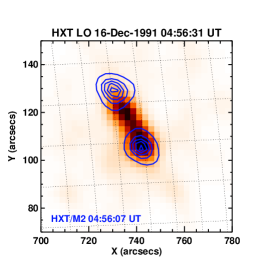
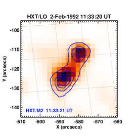
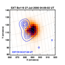
Figure 1: Images of three analysed flares taken by Yohkoh satellite with SXT or HXT/LO (gray scale images) and HXT (iso-contours) telescopes.

Most of the published observations of the solar events did not indicate a presence of a large blue-shifted component of the spectrum. However, most 1D hydrodynamic (HD) numerical models of the chromospheric evaporation in a single-loops show a presence of very high up-flow velocities, up to several hundred kilometers per second (Emslie et al., 1992; Mariska & Zarro, 1991; Mariska et al., 1993; Mariska, 1994). This discrepancy between observations and models could be explained by insufficient sensitivity of the instruments (Antonucci et al., 1987; Doschek & Warren, 2005) but most of the theoretical works present models of the solar flares having low up-flow velocities. The most advanced model of this kind is a multi-thread model of the flare proposed by Hori et al. (1998) and developed by Doschek and Warren, consistent with the observed BCS spectra (Doschek & Warren, 2005; Warren & Doschek, 2005). In this paper we present other explanation of the lack of the blue-shifted spectra. For three solar flares we show that one can well explain the observed spectra using simple 1D single-loop HD models and taking into account geometrical effects of the viewing angles to the loops.

We describe the observed flares (Sect. 2), the model calculation (Sect. 3), the obtained results (Sect. 4) and the discussion and conclusions (in Sect. 5.)

2 Observational data

We selected three solar flares observed by the Yohkoh satellite on the disk, having a clearly recognizable single-loop geometric structure and maximum hard X-ray flux not less than 10 ctns/sec per subcollimator in the M2 channel (33-53 keV) of the HXT instrument (Kosugi et al. (1991)). Two analysed flares: C2.7 GOES class flare observed on 1992 February 2 and M2.4 flare on 2000 July 27 were not mentioned previously in literature; the third one, M2.7 class flare on 1991 December 16, was investigated previously by Culhane et al. (1994). All the flares were observed with HXT telescope during their impulsive phases but only one of them (2000 July 27) was also observed with the Yohkoh SXT grazing-incidence telescope (Tsuneta et al. (1991)). HXT images of the flares were reconstructed using the standard Pixon method (Metcalf et al. (1996)) with variable accumulation times and an assumed threshold count rate of 200 counts in the M2 band (33-53 keV). The emissions of the flares were routinely recorded with the GOES X-ray photometers (1-8  Å  and 0.5-4  Å  bands). The images of the investigated flares are shown in Fig. 1, and their main characteristics are given in Table 1.

Geometrical parameters of the loops i.e. their lengths ($L_{0}$), cross-sections (S) and inclinations were evaluated under assumption that an observational error of the position of the observed structure is of the order of one pixel (i.e. 2.45 arcsec). In a course of the calculations both semi-lengths and cross-sections of the loops were refined (in a range of the error only) in order to obtain the best conformity between theoretical and observed GOES and BCS light curves (Table 1 presents final values of S and $L_{0}$ used in calculations). The errors of inclinations of the loops depends on flare localization on the Sun but for all investigated events are less than $\pm 5$ deg.

The observed X-ray spectra of the flares were recorded with the Bragg Crystal Spectrometer (BCS) instrument on board Yohkoh satellite (Culhane et al. (1991)). The BCS was a full-Sun crystal spectrometer, which measured spectra in the vicinity of strong resonance lines of H-like FeXXVI and He-like FeXXV, CaXIX, and SXV ions using curved crystals. The spectra were registered in one-dimensional position-sensitive proportional counters, with a time resolution of $<1$ sec. In this paper we used spectra measured around CaXIX resonance line. The BCS does not have the absolute wavelength calibration because locations of spectra on the detector depends on the locations of the flares on the Sun. To take account this pointing offset we determined the rest wavelengths of the spectra using spectra recorded late in the flare when expected velocities are small.

2.1 M2.7 flare on 1991 December 16

The M2.7 GOES incremental class (i.e.,background subtraction) solar flare occurred at 04:54 UT on 1991 December 16 in an active region NOAA 6961 on N04W45. The flare appeared as a single loop of moderate semi-length of about 15 400 km in SXR (see Fig. 1). The impulsive HXR emission of the flare above 23 keV was recorded between 04:55:50 UT and 04:56:28 UT. We estimated the cross-section of the loop as equal to $S=3.85\times 10^{17}$ $\rm cm^{2}$ using the reconstructed HXR images.

The BCS observations of this flare were described in detail by Culhane et al. (1994). We used spectra measured around CaXIX resonance line. The spectra were recorded in a 6 sec cadence from 04:56:06 UT except the first spectrum recorded at 04:55:42 UT with a 24 sec integration time. A blue-shifted, highly asymmetric component dominated between 04:56:06 and 04:56:48 UT. High asymmetry suggests wide spectrum of up-flow velocities.

A numerical model of the flare was calculated using parameters of the photon spectra $\gamma$ and scaling factors $a_{0}$ calculated as a function of time on the basis of hard X-ray fluxes observed in $M1$ and $M2$ channels of the HXT instrument.

2.2 C2.7 flare on 1992 February 02

The C2.7 GOES incremental class flare on 1992 February 02 was observed between 11:33 UT and 11:38 UT in an active region NOAA 7042 on S11E41 with Yohkoh/HXT and GOES only (see Fig. 1). The impulsive HXR emission above 23 keV was recorded between 11:33:18 UT and 11:33:28 UT only. HXT/LO images of the flare show X-ray emission of a single loop of moderate semi-length $\sim 9750$ km. The feet of the loop were seen in images taken in HXT channels M2 and H only. An estimated area of the loops cross-section was equal to $S=2.30\times 10^{17}$ $\rm cm^{2}$.

The CaXIX spectra were recorded from 11:33:01 UT with 6 sec cadence. The blue-shifted component with velocity higher than 200 km/s become visible 6 sec later.

The numerical model of the flare was calculated in the same way as for the previous one.

2.3 M2.4 flare on 2000 July 27

The M2.4 GOES incremental class solar flare on 2000 July 27 was observed between 04:08 UT and 04:13 UT in an active region NOAA 9090 on N10W72. The flare was visible in SXT as a single loop of moderate semi-length of about 8 690 km (see Fig. 1). The impulsive hard X-ray emission above 23 keV was recorded between 04:07:54 UT and 04:08:30 UT . We estimated the cross-section of the loop as equal to $S=2.31\times 10^{17}$ $\rm cm^{2}$ using the reconstructed HXR images.

The spectra were recorded with a 6 sec cadence starting from 04:08:11 UT except the first spectrum recorded at 04:07:47 UT with a 24 sec integration time. From beginning of the impulsive phase spectra reveal clear blue-shifted component. The blue-shifted component was highly asymmetric and dominated between 04:56:06 UT and 04:56:48 UT. This suggests wide spectrum of up-flow velocities.

The numerical model of the flare was calculated in the same way as for the previous events.

3 Method of analysis

The BCS CaXIX synthetic spectra of the investigated events were calculated using results of the 1D numerical HD models of the observed events. The HD models take into account main factors forming an energy budget and plasma kinetics of the flares: observed energy distributions of the non-thermal electrons and temporal variations of the emitted X-ray fluxes, geometry of the flaring loops estimated using images of the events, estimated main initial physical parameters of the plasma (density, temperature) and processes of gain and losses of the energy by the matter.

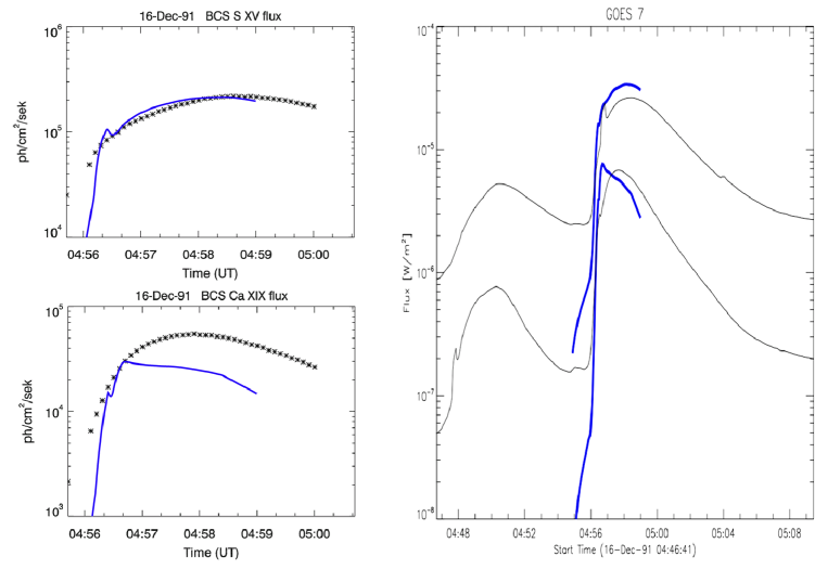
Figure 2: On the left: synthesised BCS CaXIX and BCS SXV fluxes (blue lines), and the observed ones (asterisks) of the M2.7 class solar flare observed on 16 December 1991. On the right: synthetic X-ray fluxes in 0.5-4 Å  and 1-8 Å  bands calculated using a numerical model for the same solar flare observed on 16 December 1991 (blue thick line) and relevant fluxes recorded with GOES 7 satellite (thin gray lines).

In this work we used the modified Naval Research Laboratory Solar Flux Tube Model code kindly made available to the solar community by Mariska and his co-workers ((Mariska et al., 1982, 1989)). A typical flaring loop can be modeled for many purposes with a simple 1D hydrodynamic model (as with the NRL Code) although it is a 3D structure surrounded by a complex active region. We included a few modifications to the original NRL code: new radiative loss and heating functions; the VAL-C model (Vernazza et al. (1981)) of the initial structure of the lower part of the loop (extended down using Solar Standard Model data; Bahcall & Pinsonneault (2004)), double precision of the calculations and a mesh of new values of the radiative loss function, calculated using the CHIANTI (version 5.2) software (Dere et al., 1997; Landi et al., 2006) for a temperature range $10^{4}-10^{8}$ K and density range $10^{8}-10^{14}\rm cm^{3}$. All changes were tested by comparison of the obtained results with the results of original models published by Mariska.

A sole important problem which we meet during the modeling of the flares using original NRL code was an insufficient amount of the mater located in feet of the loops. All our attempts to apply energy flux derived from observational data of medium or big-class solar flares caused massive evaporation of the whole NRL isothermal ”chromosphere” and an un-physical ”diving” of the feet, even if the chromosphere was un-realistically thick. To solve this problem we applied the VAL C model of the solar plasma, extended down using Solar Standard Model data. It was done solely in order to obtain big enough storage of the matter. Under such assumption doesn’t matter much which particular VAL model is used. All other aspects of the NRL model of the chromosphere are unchanged (radiation is suppressed, optically thick emission is not accounted for, and no account is taken of neutrals).

Main geometrical parameters of the flaring loops: the volume (V), loop cross section (S), half-length ($L_{0}$) and a local inclination of the loop’s axis to the line of sight were determined using images taken with SXT and HXT. The loop cross sections were estimated as the areas within a flux level equal to 30% of the maximum flux in the HXT/M2 channel. Loop half lengths $L_{0}$ were estimated using distances between the centres of gravity of the HXT/M2 footpoints, assuming a semi-circular shape for the loop an fixed cross-section.

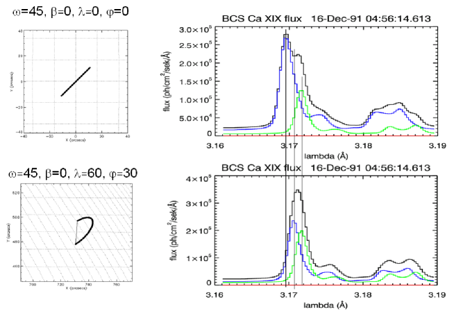
Figure 3: Influence of the position and orientation of the loop on the spectrum obtained and the observed blue-shift for the same physical and geometrical parameters of the loop. Numerically modeled BCS CaXIX spectra are plotted with solid thin lines (black), blue-shifted component of the modeled spectra are plotted with blue lines, red-shifted component with red lines and static component with green lines, respectively.

Temperatures ($T_{e}$) and emission measures (EM) of the plasma were estimated using GOES 1 - 8 Å  and 0.5 - 4  Å  fluxes and the filter-ratio method proposed by Thomas et al. (1985) and updated by White et al. (2005). Mean electron densities ($n_{e}$) were estimated from emission measures (EM) and volumes ($V=2L_{0}S$).

The heating of the plasma by the Coulomb collisions of the non-thermal electrons was modeled using the approximation given by Fisher (1989), necessary parameters of the non-thermal electron distributions were calculated as a function of time from hard X-ray fluxes observed in the HXT M1 and M2 channels. We calculated time variations of the spectral indexes ($\gamma$) and scaling factors $a_{0}$ (photon flux at 1 keV) for the impulsive phases of the investigated flares assuming power-law hard X-ray photon spectra. Electron spectra of the form of $F=A\,E^{-\delta}$ can be calculated from power-law photon spectra using the thick target approximation. A detailed description of this numerical model is also given by Falewicz et al. (2009).

All models were calculated for periods lasting from the beginning of the impulsive phase beyond the soft X-ray emissions maximum. The time steps in the models were about 0.0005-0.001 sec.

While the chromospheric evaporation is powered by non-thermal electrons, a proper estimation of the energy flux carried by electrons is decisive for realistic evaluation of the plasma velocity field. The total energy carried by the non-thermal electrons is very sensitive to the assumed low energy cut-off of the electron spectrum ($E_{c}$), due to the power-law nature of the energy distribution. A change of the $E_{c}$ value by just a few keV can add or remove a substantial amount of energy from/to the modelled system, so $E_{c}$ must be selected with great care. For investigated flares we estimated $E_{c}$ using an iterative method, selecting $E_{c}$ value which gives the best agreement of the synthesized and observed X-ray fluxes recorded with GOES X-ray photometers (i.e. GOES classes for 1-8  Å  band) and Yohkoh/BCS fluxes. Examples of the achieved conformity of the observed and synthesized BCS light curves and the observed and synthesized GOES curves are shown in Fig. 2. For each flare the selected value of the $E_{c}$ was fixed while electron spectral index ($\delta$) and corresponding scaling factor (A) varied in time in accordance with the observed variations of the HXR energy flux. The values of the $\delta$ and estimated $E_{c}$, observed at maximum of the HXR emission, are given in Table 1.

As a result of HD numerical modeling we obtain time sequences of 1D models of flaring loops. Each model consists of  2000 cells with individual $\rm T_{e}$, EM and velocity v. For each cell we calculated corresponding spectrum at vicinity of CaXIX resonance line using Chianti 5.2 emissivities for continuum and lines; each cell’s spectrum was Doppler-shifted in wavelength ($\lambda$) by $\Delta\lambda=\lambda\cdot{v}/{c}$ according to the local line-of-sight velocity component ($v$). The total CaXIX spectrum from the loop at given moment of evolution was calculated as a sum of those Doppler-shifted cell’s spectra. For better comparison with observations we used the same dispersion i.e., the wavelength bin width as obtained from BCS data.

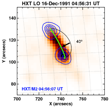
Figure 4: Image of the flare taken by Yohkoh satellite with SXT or HXT/LO (gray scale images) and HXT (iso-contours) telescopes. The theoretical semi-circular loop anchored in the footpoints and perpendicular to the solar surface (black) should be declined (tilted) 40 degrees from the vertical to cover with the observed loop (green).

Velocities projected along the line-of-sight (LOS) for each volume element (cell) of the loop were calculated in the way similar to the method described by Li et al. (1989). The LOS velocities depend on geometry of the loop, on their orientation (inclination to the solar surface ($\beta$) and the tilt angle ($\omega$)), and their heliographical coordinates ($\lambda,\phi$). In Fig. 3 we compared spectra obtained for the same velocity distribution along the loop but for two different loop positions on the solar disk. Depending on the loop location and orientation the blue-shifted component may be dominant or only small feature in the spectrum.

The inclinations of the loops to the solar surface ($\beta$) were calculated under assumptions of their semi-circular shape. Using SXT or HXT/LO images we fitted the observed loops with semi-circular loop having the same length and rooted in the same points, but inclined to the solar surface (an example is shown in Fig. 4). Using known longitudes and latitudes of the feet and inclination of the loop to the solar surface an actual projection of a velocity vector along the loop on the line of sight axis were evaluated for all points of the calculation mesh along the loop.

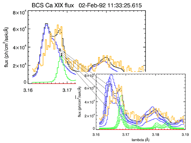
Figure 5: The observed spectrum as the sum of several spectra from the model. More details can be found in the text.

All investigated flares emitted a slightly enhanced BCS emission long before beginnings of the detected hard X-ray emissions. In order to generate a similarly enhanced BCS emissions in our numerical models of the flares we started calculations of the temporal evolution of the models tens of seconds before the beginnings of the recorded hard X-ray emissions (i.e., before beginnings of plasma heating by non-thermal electrons) applying a low energy pre-heatings fitted to mimic the observed enhancement of the BCS emissions. The values of the flux maxima are reproduced very well but the noticeably large discrepancies during the early rise and especially late decay phases are caused by a lack of additional pre- and post-impulsive heating of the plasma in our model.

The fast time variations of the energy fluxes carried by non-thermal electrons (of a sub-second time scales) cause significant changes of the temperature, density and plasma velocity distributions along the flaring loops and relevant variations of the HXR emission of the solar flares in a sub-second time scale also (e.g., Radziszewski et al. (2007)). Due to the technical features of the Yohkoh/BCS spectrometer and limited intensities of the X-ray emission of the investigated flares an effective time resolution of the recorded BCS spectra was of the order of 4-6 seconds. Thus, each recorder BCS spectrum could be recognized as a sum of numerous spectra emitted consecutively by the flaring loop in a course of the period of the spectrum’s accumulation. In order to mimic the process of observed spectra accumulation, the momentary BCS spectra calculated for consecutive time steps of the numerical models of the flares were averaged over the periods equal to the relevant periods of accumulation of the observed BCS spectra. In Fig. 5 we present an example of evolution of the synthetic spectra during accumulation period. These variations are large, both stationary and blue-shifted components can change significantly during the period when BCS collected the spectra. This fact should be kept in mind when interpreting the observed spectra. This is especially important during rise phase of the flares when, because of low statistic, an accumulation times varied from 6 up to 9 seconds.

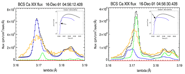
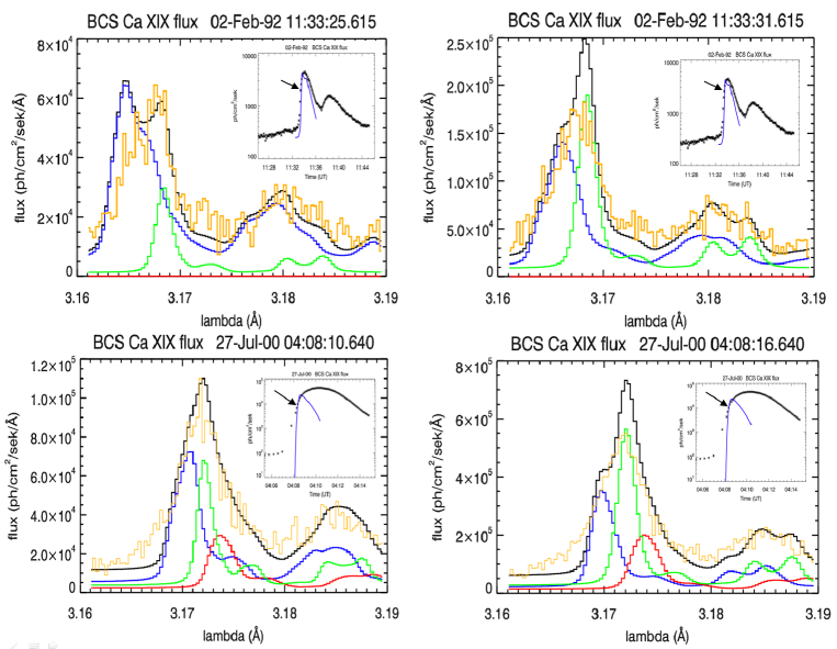
Figure 6: The observed spectrum for the different moments of time for the three analysed events. Observed BCS CaXIX spectra are plotted using solid thick lines (yellow), numerically modeled spectra are plotted with solid thin lines (black), blue-shifted component of the modeled spectra are plotted with blue lines, red-shifted component with red lines and static component with green lines, respectively.

4 Results

We defined blue-shifted, static and red-shifted components of the numerically modeled spectrum as emissions of plasma having radial velocities: greater than 50 km/s (toward the observer), between -50 km/s and 50 km/s, and greater than -50 km/s (outward the observer), respectively. The observed BCS CaXIX spectra are plotted using solid thick (yellow) lines, numerically modeled spectra are plotted with solid thin lines (black), blue-shifted component of the modeled spectra are plotted with blue lines, red-shifted component with red lines and static component with green lines, respectively (see Fig. 6).

4.1 M2.7 flare on 1991 December 16

The flare appeared in SXR as a single loop with semi-length 15 400 km inclined to the local vertical direction by 40 deg (see Fig. 1, left panel and Fig. 4). BCS observations revealed the strong and highly asymmetric blue-shift component recorded from beginning of impulsive phase. High asymmetry of the spectral lines indicated wide spectrum of up-flow velocities.

The numerical model of the flare was calculated for the period lasting from 04:54:52 UT to 04:58:52 UT (240 sec), which covers an impulsive phase of the flare and spreads beyond maximum of the recorded GOES satellite emission.

The blue-shifted emission is less than or comparable to the stationary component only on the first observed spectrum. The time evolutions of the synthetic and observed BCS CaXIX spectra are very similar. The synthetic spectrum consists of the static component only up to 04:56:00 UT. The blue-shifted emission appeared at 04:56:00 UT and increased instantly, but up to 04:56:08 UT it is dominated by the static component. After that the spectrum was dominated by broadened blue-shifted emission entirely. The observed (yellow) and synthetic (black) spectra recorded between 04:56:12 UT and 04:56:18 UT (6 sec accumulation time) as well as blue-, red- and stationary (green line) components of the synthetic spectra are shown in Fig. 6 upper-left panel. While blue-shifted synthetic component is narrower then much more dispersed observed one, the overall agreement between model and observations seems to be fulfilled. The blue-shifted emission diminished gradually after 04:54:30 UT. Faint red-shifted emission appeared in the synthetic spectra between 04:56:24 UT and 04:56:29 UT. In Fig. 6 (right panel) we compared the observed and synthetic spectra for the period (between 04:56:30 UT and 04:56:36 UT with 6 sec accumulation time). Again, the qualitative agreement between theory and observations is good. Blue-shifted component vanished entirely after 04:56:46 UT ($\sim 20-30$ sec earlier than observed), and BCS CaXIX spectrum became static again.

4.2 C2.7 flare on 1992 February 2

HXT/LO images of the flare show the X-ray emission arriving from a single loop with semi-length $\sim 9750$ km, inclined to the local vertical direction by 35 deg (see Fig. 1, central panel).

The numerical model of the flare was calculated for the period from 11:32:32 UT to 11:35:57 UT (205 sec), covering an impulsive phase and spreading beyond maximum of the emission recorded with GOES. Stationary component was present in both synthetic and observe spectra up to 11:33:01 UT only . There is a good compliance between modeled and observed spectra although the registered signal was weak. After 11:33:13 UT the blue-shifted component with velocity v$\sim 250$ km/s appeared in the spectra. Initially weak, this component increased instantly.

The blue-shifted component dominated after 11:33:19 UT the stationary one. The velocity of blue-shifted component was about v$\sim 220$ km/s. There is good agreement between model and observe spectra (see Fig. 6 - left panel, where the color line markings are the same as in earlier events). The stationary component dominates from 11:33:31 UT again and mean velocity of the blue-shifted component decreased to v$=190$ km/s. The time evolutions and shapes of synthetic and observed spectra match well. The blue-shifted emission in the modeled spectrum diminished after 11:33:36 UT gradually, vanishing entirely at 11:33:43 UT, when the synthetic BCS CaXIX spectrum became static again. No red-shifted emission was present during the whole modeled period of the flare’s evolution.

4.3 M2.4 flare on 2000 July 27

The flare was visible in SXT as a single loop perpendicular to the solar surface (see Fig. 1, right panel) with semi-length $\sim 8690$ km.

The numerical model of the flare was calculated for the period from 04:07:56 UT to 04:10:30 UT, covering an impulsive phase and maximum of the emission recorded with GOES. The observed BCS CaXIX spectra include blue-shifted and stationary components up to 04:07:46 UT. The blue-shifted component with velocity v = 180 km/s (which is two times weak than stationary) can be seen in the observed spectra. The model agrees well with the observed spectra although the observed lines are more broadened that the ones in the model. The blue-shifted component with velocity v$=290$ km/s dominates in the spectra after 04:08:10 UT. There is a good compliance between modeled and observed spectra. In this time also a faint red-shifted emission was present on the synthetic spectra (Fig. 6 - left panel, the color of the lines are the same as in earlier events). After 04:08:16 UT the stationary component begins to dominate again and velocity of blue component decreased (v=120 km/s), until complete disappearance (see Fig. 6 - right panel). A faint red-shifted emission was still present on the synthetic spectra. After 04:08:43 UT the synthetic BCS CaXIX spectrum become static again.

5 Discussion and conclusions

Numerical modeling of the flares allows to study distributions of the plasma velocities along the flaring loops. Thus, it is possible to estimate relative contributions of the emissions of the stationary and moving plasma to the spectra (i.e. their stationary and shifted components).

Most of papers describing results of the analysis of the BCS data indicate that the BCS spectra are dominated by stationary component. Additionally, there is only a very limited number of described observations of the solar flares having spectra in which the blue-shifted component dominates the stationary one. The statistical paper by Gan and Watanabe shows that although moderate blue asymmetry is very common during the impulsive phase, the number of events having spectra with great blue-shift is very small. They also found that for most flares the blue-shift emission appears during early impulsive phases and is temporally correlated with the line broadening.

Most 1D numerical models of the chromospheric evaporation in single-loops show a presence of very fast up-flows, up to several hundred kilometers per second. This discrepancy between observations and models could be explained by insufficient sensitivity of the instruments but most of the theoretical works present models of the solar flare having low up-flow velocities. The most advanced model of this kind is a multi-thread model of the flare proposed by Hori and co-workers and developed by Doschek and Warren, consistent with the observed BCS spectra. In this paper we present other explanation of the lack of the observed blue-shifted spectra.

We investigated C2.7 GOES class flare observed on 1992 February 2, M2.4 flare observed on 2000 July 27, and M2.7 class flare observed on 1991 December 16. Two of the analyzed flares (C2.7 and M2.4) were not described previously in literature; the third one, M2.7 was investigated by Culhane et al. (1994). The synthetic BSC spectra of the flares were calculated using real observational parameters of the observed flares (geometry, physical parameters of the plasma, energy spectrum of the non-thermal electrons).

For all investigated events we obtained good quantitative conformability of the synthetic and observed BCS CaXIX spectra. For the whole impulsive phase of each flare we obtained overall good agreement of fluxes, shapes and time variations of the observed and synthetic spectra.

Generally, widths of the observed spectral lines were greater than widths of the relevant synthetic spectra lines. The observed blue-shifted component was wider than synthetic one and highly asymmetric. This suggests wider dispersion of up-flow velocities in observed events than in our theoretical models. This non-conformability could be caused by disregarded turbulent motions of the plasma in our numerical model and by some differences between calculated and real distributions of the physical parameters of the plasma along the loops (densities, temperatures, and macroscopic velocities). Nevertheless, we obtained good conformity between overall shape, stationary, red- and blue-shifted components of the relevant calculated and observed spectra.

Despite very high up-flow velocities of the plasma obtained in numerical simulations of the various flares similarly high radial velocities could be observed mostly for the events located in the central part of the solar disc only, due to a geometrical projection of the velocity vector onto the direction of sight. Assuming a semi-circular loop located perpendicularly to the local solar surface and rooted at the solar longitude of 60 deg the LOS component of the velocity is two times smaller than the real velocity of the plasma along the loop. Similarly about 50% of the emission emitted as blue-shifted from the loop rooted at the disc centre is observed as a stationary component for the loop rooted at the solar longitude of 60 deg. So, taking into account the geometrical dependences of the LOS velocities of the plasma moving along the loops inclined toward the solar surface as well as a distribution of the flare sites over the solar disc we can conclude that stationary component can be observed for all flares during their early phases of evolution (i.e., in almost all flares exist some plasma which don’t move along the LOS). On the other side, the blue-shifted component of the spectrum could be not detected even for plasma rising along the flaring loop with very high velocity. Additionally our simulations based on realistic heating rates by non-thermal electrons indicate that the upper chromosphere plasma is heated by non-thermal electrons a few seconds before beginning of noticeable high-velocity bulk motions, and until this time its emits stationary (not red- or blue-shifted) spectrum only.

Very similar investigations of the impact of the various viewing angles on the resulting spectral signature of the flare was made already by Li et al. (1989). Li and co-workers used theoretical models of flaring loops with arbitrary selected plasma parameters and temporal variations of the local heating. For most cases they obtained a strong blue-shifted component of the spectrum. Our models are based on observational data; especially duration of the heating and delivered energy flux were evaluated from HXT/Yohkoh data. In our models the absolute velocities of the plasma up-flow were of the order of 450-500 km/s, but taking into account the geometrical effect of the angle of view on the loops they were reduced to moderate 200-250 km/s.

Taking into account the geometrical dependences of the line-of-sight velocities of the plasma moving along the flaring loop inclined toward the solar surface as well as a distribution of the investigated flares over the solar disk, we conclude that stationary component of the spectrum should be observed almost for all flares during their early phases of evolution. In opposite, the blue-shifted component of the spectrum could be not detected in flares having plasma rising along the flaring loop even with high velocity due to the geometrical dependences only. Our simulations based on realistic heating rates of plasma by non-thermal electrons indicate also that the upper chromosphere is heated by non-thermal electrons a few seconds before beginning of noticeable high-velocity bulk motions, and before this time plasma emits stationary component of the spectrum only. After the start of the up-flow motion, the blue-shifted component dominate temporally the synthetic spectra of the investigated flares at their early phases.