Diamonds on the Hat: Globular Clusters in The Sombrero Galaxy (M104)¹

Abstract

Images from the Hubble Space Telescope Advanced Camera for Surveys are used to carry out a new photometric study of the globular clusters (GCs) in M104, the Sombrero galaxy. The primary focus of our study is the characteristic distribution function of linear sizes (SDF) of the GCs. We measure the effective radii for 652 clusters with PSF-convolved King and Wilson dynamical model fits. The SDF is remarkably similar to those measured for other large galaxies of all types, adding strong support to the view that it is a “universal” feature of globular cluster systems.

We use the Sombrero and Milky Way data and the formation models of Baumgardt & Kroupa (2007) to develop a more general interpretation of the size distribution function for globular clusters. We propose that the shape of the SDF that we see today for GCs is strongly influenced by the early rapid mass loss during their star forming stage, coupled with stochastic differences from cluster to cluster in the star formation efficiency (SFE) and their initial sizes. We find that the observed SDF shape can be accurately predicted by a simple model in which the protocluster clouds had characteristic sizes of $0.9\pm 0.1$ pc and SFEs of $0.3\pm 0.07$.

The colors and luminosities of the M104 clusters show the clearly defined classic bimodal form. The blue sequence exhibits a mass/metallicity relation (MMR), following a scaling of heavy-element abundance with luminosity of $Z\sim L^{0.3}$ very similar to what has been found in most giant elliptical galaxies. A quantitative self-enrichment model provides a good first-order match to the data for the same initial SFE and protocluster size that were required to explain the SDF.

We also discuss various forms of the globular cluster Fundamental Plane (FP) of structural parameters, and show that useful tests of it can be extended to galaxies beyond the Local Group. The M104 clusters strongly resemble those of the Milky Way and other nearby systems in terms of such test quantities as integrated surface density and binding energy.

1 Introduction

Our knowledge of globular cluster (GC) systems in spiral and disk galaxies is far more limited than those in elliptical galaxies, and consists primarily of the samples in the Milky Way and in M31, along with a handful of more distant disk galaxies (Kissler-Patig et al., 1999; Goudfrooij et al., 2007; Chandar et al., 2004; Rhode et al., 2007; Spitler et al., 2006; Mora et al., 2007; Cantiello et al., 2007; DeGraaff et al., 2007). These should be compared with the many extensive studies of the GC systems in elliptical galaxies, particularly the giant E’s in which GCs can be found by the thousands (e.g. Larsen et al., 2001; Brodie & Strader, 2006; Peng et al., 2006; Harris, 2009a, to name only a few). But if we are to probe the systematic properties of the GCs themselves and to understand further the common nature of these classically ancient objects, we need to investigate them closely across all types of host galaxies.

The Sombrero galaxy (M104 = NGC 4594), a giant Sa system, is the disk galaxy with the largest known population of globular clusters (GCs) and for that reason alone is a particularly attractive system. The fact that it is distinctly closer ($d=9$ Mpc) than the Virgo cluster, and also nearly edge-on to our line of sight so that our view of its GC population is minimally affected by issues of reddening and contamination from the disk itself, makes M104 an almost unique target. Rhode & Zepf (2004), from wide-field ground-based imaging, derive a total GC population of 1900 clusters. They find that the spatial extent of the system is at least as large as 40 kpc in projected galactocentric distance.

In an earlier study (Spitler et al., 2006, which we refer to as Paper I), a first round of HST-based photometry of M104 GCs and measurements of their scale sizes was presented. Chandar et al. (2007) used the same material to evaluate the trend of mean GC density with galactocentric distance. The raw data consisted of a special imaging dataset of six fields taken with the ACS Wide Field Channel as part of a Hubble Heritage Project on M104 (PI: K. Noll, PID 9714). This mosaic was observed in the standard $BVR$ filters (F435W, F555W, F625W) and covers a total field size of about $600^{\prime\prime}\times 400^{\prime\prime}$ centered on M104. In Paper I, photometry from the individual images was used to discuss the distribution of the GCs in luminosity and color, their spatial distributions around the galaxy, the differences between the red (metal-rich) and blue (metal-poor) GC subsystems, and the correlations of cluster sizes with GC luminosity and galactocentric distance. In addition, Paper I also provided the first indication that the metal-poor GCs in disk galaxies showed a correlation between mass and metallicity that had already been uncovered for elliptical galaxies.

In the present study, we use the reprocessed mosaic of ACS images to measure the GCs in M104. A particular emphasis of this study is the use of newer algorithms to take a deeper look into the intrinsic scale sizes of the GCs, and carry out a more extensive set of comparisons with other galaxies. This work leads us into a physical model for the origin of the GC size distribution that we observe today.

In Section 2 we describe in detail the photometry and size measurements. In Section 3, we discuss the correlations of GC scale size with luminosity, metallicity, and galactocentric distance, and show that versions of the “Fundamental Plane” of structural parameters can be accurately constructed for GCs in galaxies this distant. In Section 4, we introduce a quantitative model for the physical origin of the GC size distribution. The present-day GC size must be the result, not only of the slow dynamical evolution of the cluster in the tidal field of the galaxy, but also of the expansion of the protoclusters during their early phase of star formation and rapid gas expulsion. The key parameters in this model are the original protocluster size, the star formation efficiency, and (just as importantly) the dispersions in these two quantities. Finally, in Section 5 we redetermine the correlations of GC color (metallicity) with luminosity for both the bimodal sequences with our new photometry. We conclude more strongly than before that this galaxy has a mass/metallicity relation quite similar to those in the giant ellipticals. Section 6 gives a brief summary of our findings. (Readers interested primarily in the results may skip directly to Section 3 without loss of continuity.)

Throughout this paper, we adopt the distance modulus $(m-M)_{0}=29.77$ ($d=9.0$ Mpc; see Table 4 in Paper I) along with a foreground reddening $E_{B-V}=0.05$ from the NASA/IPAC Extragalactic Database (NED). At the adopted distance, the image scale is 1 pixel $=0.05^{\prime\prime}=2.2$ parsecs.

2 Goals of the Study

The most prominent focus of the present discussion is the characteristic scale size of the GCs (the effective or half-light radius, denoted $r_{h}$). We refer to the distribution function of their sizes (effective radii) as the SDF. At the 9-Mpc distance of M104, a GC with a typical size $r_{h}\simeq 3$ pc subtends an angular diameter of about $0.14^{\prime\prime}$, which is similar to the ACS/WFC point-spread function width of FWHM $0.1^{\prime\prime}$. In the sense defined by Harris (2009a), the clusters are therefore in the partially resolved regime: their individual profiles are easily distinguished from stars, and their effective radii are clearly measurable. Extensive tests of GC profile-fitting for galaxies ranging out to distances of $\sim 50$ Mpc show that GC effective radii can be accurately measured as long as the stellar PSF is precisely known and the cluster size $r_{h}$ is no smaller than about 10% of the PSF fwhm (Kundu & Whitmore, 1998; Larsen, 1999; Jordán et al., 2005; Georgiev et al., 2009; Harris, 2009a). As will be seen below, the clusters in M104 are far above this resolution limit.

We use our new measurements to establish the SDF more accurately, and to define the “Fundamental Plane” of GC structural parameters in comparison with other galaxies. The half-mass radius $r_{h,m}$ is an interesting and important quantity for GC dynamics because it remains relatively constant over many internal relaxation times (e.g. Spitzer & Thuan, 1972; Aarseth & Heggie, 1998; Baumgardt et al., 2002; Trenti et al., 2007) and thus represents an intrinsic scale size that was established closer to its formation time. As we will discuss in Section 4 below, the physical origin of the SDF is likely to be sensitively dependent on a combination of the star formation efficiency (SFE) and the original scale size ($r(init)$) of the protoclusters. The fact that the SDF has a near-universal form among globular cluster systems can then be turned around to place surprisingly close limits on the SFE and $r(init)$.

The HST cameras, beginning with WFPC2, have provided the key instrumental tools that have allowed us to resolve GCs in galaxies well beyond the Local Group and to measure their scale sizes accurately. Pioneering work of this type began a decade ago (Kundu & Whitmore, 1998, 2001; Kundu et al., 1999; Larsen, 1999; Larsen et al., 2001) and the changeover from WFPC2 to the ACS camera soon led to faster gains and large databases of cluster sizes (e.g. Jordán et al., 2005, 2009; Harris, 2009a). These surveys of resolved GC populations have started to reveal that $r_{h}$ also depends weakly on three other cluster properties. First of these is a gradual increase in mean $r_{h}$ with galactocentric distance (Hodge, 1962; Mateo, 1987; van den Bergh al., 1991; Jordán et al., 2005; Spitler et al., 2006; Cantiello et al., 2007; Gómez & Woodley, 2007; Harris, 2009a; Madrid et al., 2009). This trend is generally interpreted as the result of the weaker external tidal field of the host galaxy with increasing distance (see von Hoerner, 1957; King, 1962; van den Bergh al., 1991; Murray & Lin, 1992; Harris & Pudritz, 1994; Baumgardt & Makino, 2003), raising the intriguing possibility that the GC sizes can provide a tracer of the galaxy potential well independently of other approaches.

Secondly, in most galaxies a detectable difference in mean size with cluster metallicity has been found, with the red GCs being typically 15-20% smaller than the blue ones (Kundu & Whitmore, 1998; Kundu et al., 1999; Larsen et al., 2001; Jordán et al., 2005; Gómez & Woodley, 2007; Harris, 2009a, and Paper I). This second trend has been variously interpreted as (a) a geometric-projection byproduct of the fact that the metal-richer clusters usually lie in a more centrally concentrated spatial distribution than the metal-poor ones, coupled with the growth in mean $r_{h}$ with $R_{gc}$ (Larsen & Brodie, 2003); (b) a result of metallicity-dependent stellar evolution times and dynamical mass segregation within the clusters (Jordán, 2004); or (c) a residual of the cluster formation epoch, in which the gas within a metal-richer protocluster could cool and collapse further than in a metal-poor one before forming stars (Harris, 2009a). Combinations of these effects are of course not ruled out.

A third empirically established trend is the correlation of GC scale size with cluster luminosity or mass. Even though there is obvious cluster-to-cluster scatter in intrinsic sizes, their median scale size differs little with absolute magnitude from a global value of $2.5-3$ pc (e.g. Jordán et al., 2005; Barmby et al., 2007). It is only at the high-luminosity end ($\sim 5\times 10^{5}$ Solar masses and above) that a trend towards somewhat larger $r_{h}$ seems to emerge. This mass/radius relation may, possibly, bridge the sequence of normal GCs to other kinds of compact stellar systems such as UCDs (Ultra-Compact Dwarfs) that have scale sizes of typically $\sim 10-30$ pc (Hasegan et al., 2005; Kissler-Patig et al., 2006; Barmby et al., 2007; Evstigneeva et al., 2008; Harris, 2009a). These somewhat more massive compact systems (variously called UCDs, Dwarf-Globular Transition Objects (DGTOs), or Intermediate-Mass Objects (IMOs); see Forbes et al., 2008) obey a different scaling rule $r_{h}\sim M^{0.8}$ or higher (see Forbes et al., 2008; Evstigneeva et al., 2008). Globular clusters luminous enough to lie in this intriguing transition region of $10^{6}-10^{7}M_{\odot}$ are so rare that it is not yet clear whether there is a “universal” mass/radius relation for them, or what its detailed form is.

For all the reasons outlined above, high-quality measurements of GC scale sizes and structural parameters are of great value. Because of its proximity and large GC population, M104 provides one of the few best opportunities for this kind of measurement outside the Local Group.

2.1 The Data and the Profile Models

Preprocessing of the raw image data is described in Paper I. The mosaics of six pointings in each filter were constructed at STScI and are publicly available. Paper I also lays out in detail the selection of the many hundreds of individual GCs in M104 field and rejection of contaminating non-GCs scattered across the field. The contaminants are mostly small, faint background galaxies, but also include any starlike objects ($r_{h}=0$) according to the profile fits. Selection also included the use of color, magnitude, and the distribution of objects in a similar control field. There are some 658 identified high-probability GCs brighter than $R=24(M_{R}\simeq-5.8)$ plus one UCD in the final selected list, and we start the present paper with that list in hand.

In Paper I, the ISHAPE code of Larsen (1999) was used to determine the GC effective radii through convolution of King (1962) model profiles with the stellar PSF. In each of the six original ACS/WFC fields a single mean PSF was defined, and a profile with a central concentration parameter $c=r_{t}/r_{c}=30$ was adopted. For each individual cluster the intrinsic profile width $r_{h}$ (in practice, the fwhm) is varied until a best fit between the convolved profile and the real GC is obtained.

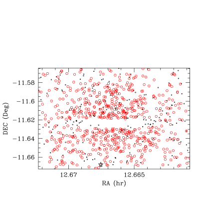
Figure 1: Location of the target objects within M104 mosaic field, which has dimensions $600^{\prime\prime}\times 400^{\prime\prime}$. The 659 GC candidates are shown as open circles, while the 179 stars used for the PSFs are marked as small dots. The large star at bottom shows the location of the UCD (Hau et al., 2009).

The ISHAPE code is a well tested and fast method for obtaining useful $r_{h}$ distributions for large samples of partially or marginally resolved objects (see, e.g. Larsen, 1999; Larsen et al., 2001; Georgiev et al., 2009; Harris, 2009a; Madrid et al., 2009). However, it does not easily handle situations where the PSF may depend on position on the image, and at a more fundamental level it uses only analytic fitting functions to describe the GC profiles. Although the King (1962) function was constructed to match real GCs in the first place, it does not capture the full range of actual profile shapes for GCs, UCDs, and related objects.

For the present work, we use the profile-fitting code of McLaughlin et al. (2008). This code has been applied previously to GCs in the Milky Way, the Magellanic Clouds, M31, and NGC 5128 (McLaughlin & van der Marel, 2005; Barmby et al., 2007; McLaughlin et al., 2008). For the intrinsic GC profile, this algorithm can employ either the King (1966) or Wilson (1975) profiles, both of which are true dynamical models constructed from simple but realistic assumptions about the energy distribution function of the stars within the cluster. In the discussion below, we refer to these models as “K66” and “W75”. Although these non-analytic models require a much larger investment in computing time, their best-fit solutions lead immediately to physically relevant quantities such as relaxation times, mean densities, binding energies, and fundamental-plane parameters (McLaughlin & van der Marel, 2005; McLaughlin et al., 2008).

A roughly similar code (KINGPHOT) has been used for GCs in the Virgo galaxies (Jordán et al., 2005, 2009; Peng et al., 2009). Although the King model is quite familiar in the literature and describes most real GCs satisfactorily, the Wilson model has some distinct advantages in its ability to handle real clusters that have symmetric but radially extended light profiles which (within the confines of the King model) would nominally be thought to have “extra-tidal light”. As is extensively discussed by McLaughlin & van der Marel (2005) and McLaughlin et al. (2008), the key difference in the Wilson model is its smoother ramp-down of the stellar energy distribution function towards higher energies, which can handle relatively larger numbers of stars near the escape energy and a more extended envelope with a nominally larger tidal radius.

It is important to note that for small to moderate radii within the cluster (that is, out to a few $r_{h}$), both the King and Wilson models give very similar profile shapes and do equally well at fitting most real clusters. These inner regions are populated by the low-energy stars far inside the tidal (escape) radius where the difference in the energy distribution function between the two models is small. For the clusters in the nearby Local Group galaxies where the profiles can be thoroughly sampled over large radii, the Wilson model often performs better, but (as is shown in McLaughlin & van der Marel, 2005; McLaughlin et al., 2008) there is no blanket ruling; decisions are made on a cluster-by-cluster basis.

The Sombrero ACS mosaic field does, however, offer a particularly vivid case where there is a strong difference between these two models. There is a single clearly identifiable luminous UCD belonging to the galaxy, whose profile has an extended outer envelope which is accurately fit by the Wilson model but where the King model completely fails. We have discussed this special object in detail in Hau et al. (2009). In the present study, we apply both of these two dynamical model profiles to the complete sample of GCs in the galaxy and explicitly compare their quality of fit.

2.2 Measurement of Cluster Profiles

The profile-fitting code is the same one described fully in McLaughlin et al. (2008). For each object, a stellar PSF (either an analytic function or an empirical numeric profile) is convolved with the K66 or W75 model, and the model parameters are adjusted until the convolution fits the observed surface brightness profile of the cluster. We carried out all the measurements on the complete wide-field mosaic for the entire field, rather than the six individual fields as in Paper I. The measurements were done from smoothed (median-filtered) images in each filter with the large-scale light gradients removed. A $31\times 31$ px box filter was used for the median filtering. We then used stsdas/ellipse to measure the radial profile for each GC in our list, out to a radius determined by the point past which the GC surface brightness fell well below the sky noise; this limit ranged from $\ga 0.5^{\prime\prime}$ for the most luminous objects to $0.1^{\prime\prime}$ for the very faintest ones.

To define the PSF profile that needs to be paired up with each GC, we chose here to select the nearest star to each individual GC, as we did in Hau et al. (2009). In this way we circumvent trying to model the small but potentially complex variation in PSF properties across the complete mosaic of six ACS fields. The stars are, in turn, empirically defined as those objects in our Paper I study that turned out to have negligible intrinsic widths ($r_{h}=0$). We drew the PSF stars from a candidate list of 179 stars with sufficiently high S/N, so the average projected separation between any one GC and its accompanying PSF star is $\simeq 20^{\prime\prime}$. The profiles of the stars were also measured through stdas/ellipse with the same parameters, and each GC/PSF pair was then run through the fitting code to find the best-fit solutions. The locations of the 658 target GCs and one UCD measured previously, along with the 179 candidate PSF stars, are shown in Figure 1. As is evident from the figure, we deliberately avoid the parts of the galaxy projected on or near the plane of the disk, where the profile fits would be badly compromised by complex background light gradients and crowding.

Lastly, we re-derive integrated magnitudes $B,V,R$ for all the GCs with aperture photometry individually adjusted for cluster profile width. The approach we use is similar in principle to Harris (2009a), where in this case we start with a fixed-aperture magnitude measured through 5 px radius ($0.05^{\prime\prime}$) and then apply a magnitude correction to “large” radius (20 px) $\Delta m=m_{5}-m_{20}$ that depends in turn on the cluster’s scale size $r_{h}$. By direct comparison of the aperture magnitudes from ISHAPE through these two apertures (Figure 2), we find that $\Delta m$ increases nearly linearly with log ($r_{h}$),

$$\Delta m\,=\,0.12\,+\,0.41{\rm log}r_{h}$$

and does not differ significantly with bandpass. Thus the aperture corrections have no significant influence on the cluster colors (see also Harris, 2009a; Jordán et al., 2009; Peng et al., 2009).

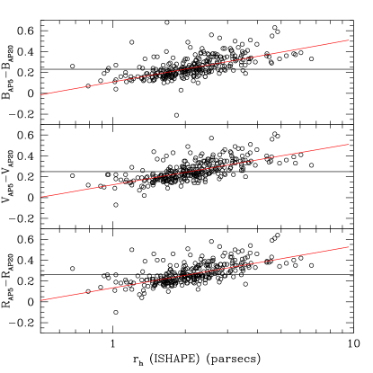
Figure 2: Empirical aperture corrections to the cluster magnitudes. The mean line through each set of points is given by the equation in the text.

Table 1: Photometry and Structural Parameters for Globular Clusters in M104

ID	RA	DEC	$R^{{}^{\prime}}_{gc}$	$V$	$B-V$	$B-R$	$r_{h}$(pc)	$\pm$(pc)	$c$	$\pm$
1	12.669456	-11.639086	2.777	18.74	0.77	1.26	3.62	0.18	1.73	0.09
2	12.669275	-11.642228	2.703	18.87	0.83	1.34	5.05	0.06	1.90	0.01
3	12.666692	-11.602536	1.243	18.83	0.76	1.27	3.72	0.46	2.37	0.71
4	12.670719	-11.641109	3.874	18.83	0.84	1.36	4.70	0.36	1.94	0.22
5	12.669567	-11.610695	2.804	18.99	0.80	1.31	3.57	0.10	1.98	0.06

The output quantities from the profile fitting code that are of primary interest here are the effective radius $r_{h}$ and its uncertainty $\sigma(r_{h})$; the central potential parameter $W_{0}$ or equivalently the concentration $c$ and its uncertainty ($c\equiv{\rm log}(r_{t}/r_{c})$ where $r_{t},r_{c}$ are the tidal and core radii); and a goodness of fit $\chi^{2}$. As all other authors have found who have worked on GC size measurements for distant galaxies (e.g. Kundu & Whitmore, 1998, 2001; Larsen, 1999; Jordán et al., 2005; Georgiev et al., 2009; Harris, 2009a), we find that the central-concentration parameter $W_{0}$ or $c$ is not very precisely determined from the best-fit solutions. The reason for this is simply that relatively small numbers of pixels are available for the code to use for the profile fit relative to the PSF size. In turn, some of the other structural quantities calculated from $c$ and $r_{h}$ (such as the cluster core radius $r_{c}$, which is far smaller than the resolution limit imposed by the PSF) will not be reliable. Empirically, we can gauge how reliable our $c-$values are by comparing the output values from the three different filters for the same object. These comparisons show that the internal consistency differs widely from one cluster to another, but has a median uncertainty near $\sigma(c)=\pm 0.4$.

Fortunately, by far the most robust quantity in the solutions is the effective radius itself. As is discussed further elsewhere (see the references cited above), $r_{h}$ is relatively insensitive to changes in $c$ in either direction because, for GCs at distances in the $\sim 5-50$ Mpc range, it sits near what is essentially a “best” point in the profile: it is neither buried in the unresolved core of the cluster, nor lost in the noise blanketing its faint outermost envelope. As long as the PSF profile is accurately known, any error in $c$ is compensated by adjustments in the total profile shape to give the well determined radius enclosing half the light. Fortunately, the M104 clusters sit well above the empirical resolution limit of $r_{h}\sim 0.1fwhm(PSF)$ below which any leverage on the structural parameters is lost.

A direct comparison of the K66 and W75 models is shown in Figure 3. Here, as in McLaughlin et al. (2008) we use a normalized $\chi^{2}$ ratio defined as $(\chi^{2}_{K}-\chi^{2}_{W})/(\chi^{2}_{K}+\chi^{2}_{W})$ where $\chi_{K},\chi_{W}$ are the values from the King and Wilson fits respectively. For most of the clusters, the values of this ratio scatter near zero, indicating that both models do about equally well at matching the real profiles. Overall, there is a slight preponderance for the W75 models to match better (positive values in the graphs) but no major differences or obvious trends with magnitude are evident. By plotting the same goodness-of-fit ratio against projected galactocentric distance $R_{gc}$, we test for any trends versus background sky noise (the large bulge of M104 becomes considerably brighter at small $R_{gc}$), but we find no systematic trends there either.

Figure 3: Left panel: Normalized $\chi^{2}$ ratio plotted versus $R$ magnitude, for the three bandpasses $BVR$. In this plot, postive values indicate that the Wilson (1975) model is preferred to the King (1966) model, while values near zero indicate that both are equally good. Right panel: Normalized $\chi^{2}$ ratio plotted against projected galactocentric distance.

Final successful profile fits and radius measurements for 652 clusters were obtained. Table 1 lists the results giving in successive columns a running ID number; right ascension and declination; projected galactocentric distance in arcminutes; $V,B-V$, and $B-R$; the mean $r_{h}$ over all three filters and its uncertainty; and the mean King central concentration parameter $c$ and its internal uncertainty. The complete version of the table is available in the electronic edition. In Figure 4, we show several solutions to individual clusters with the K66 model and drawn from the $R-$band filter.

Figure 4: Some sample profile fits with the King (1966) model for six of the clusters, ranging from the brightest in the list to the faintest (top to bottom). Dots are the measured surface brightnesses from stsdas/ellipse, while solid lines are the PSF-convolved K66 model solutions. The dashed line at bottom shows one of the PSF profiles.

2.3 Measurement Uncertainties and Error Budget

The measurement uncertainties on the $r_{h}$ values were evaluated with a series of tests. First of these was the internal consistency in the size measurement among the three filters. This comparison is shown in Figure 5, for both the K66 and W75 models. In principle, the three filters give three independent measurements of the same quantity $r_{h}$ for the same cluster (and for exactly the same PSF star), with random scatter due only to the internal uncertainty of the fit. We find good systematic agreement amongst the filters; all three correlations scatter closely along the 1:1 lines, so we make no systematic corrections between filters. However, the K66 model fits (right panels in the figure) show slightly smaller scatter, fewer outliers, and thus higher internal consistency than the W75 model.

In the end, we find little to choose between these two competing models for most individual clusters. Because of its slightly superior internal consistency (Figure 5), we adopt our results from the K66 model for the analysis and discussion following in the later sections. The K66 reductions also allow easier comparison with characteristic-size GC data from other galaxies, which we use in the later sections. As is discussed above, the W75 model becomes most effective for GCs that happen to have extended, low-surface-brightness envelopes, which would become noticeable only beyond our radial measurement limit of $\simeq 0.5^{\prime\prime}\simeq 20$ pc, and even then only for the most luminous clusters whose envelopes would be detectable above the sky noise. Higher-S/N data than we have at present will be needed to trace these outer parts for most clusters (with the notable exception of the UCD discussed above).

Figure 5: Left panels: Comparison between the cluster sizes measured in the three different filters, as measured from the Wilson 1975 model (upper panel is $B$ vs. $R$, lower panel is $V$ vs. $R$; all scales are in parsec units). Right panels: Same internal comparison for the measurements with the King (1966) model.

To obtain a final set of $r_{h}$ values, we took an unweighted average of the measurements in all three filters and calculated the uncertainty of the mean as equal to $\sigma(r_{h})=\{\sum(r_{hi}-\langle r_{h}\rangle)^{2}/n(n-1)\}^{1/2}$. The distribution of these uncertainties is shown in Figure 6, along with their dependence on $R$ magnitude. As expected, the average $\sigma(r_{h})$ increases for fainter objects due to lower S/N and the increased relative effect of background noise. The median uncertainty over the entire dataset is $\pm 0.20$ pc.

Figure 6: Upper panel: Histogram of uncertainty $\sigma(r_{h})$ in cluster effective radius returned by the model fit, in parsec units. Lower panel: Fitting uncertainty versus cluster brightness. The median uncertainty of 0.20 pc is shown as the dashed line.

Next, in Figure 7, we show the difference in the average cluster size $\Delta r_{h}=(r_{h}({\rm K66})-r_{h}({\rm W75}))$ as functions of cluster size and brightness. The median $\Delta r_{h}$ is 0.02 pc, indicating no important systematic difference between the two models over the entire range of the data. There is a slight tendency for $\Delta r_{h}$ to vary nonlinearly with either size or brightness. However, these trends fall within the internal scatter, and the most obvious interpretation is simply that at some level, we reach the irreducible “floor” where the fundamentally different assumptions built into the different models can lead to slight differences in the best-fit structural parameters. These parameters are unavoidably model-defined, and at this level the question about which solution represents the “true” cluster size becomes moot. In general, we take this graph as useful primarily for estimating the internal uncertainty of the fit because of the model assumptions alone. This fitting uncertainty per cluster (which we adopt as the rms scatter in the graph) is then $\pm 0.21$ parsec.

Figure 7: Left panel: Difference between the cluster sizes $\Delta r_{h}=(r_{h}({\rm King})-r_{h}({\rm Wilson})$ plotted versus size. Both scales are in pixel units (1 px = $0.05^{\prime\prime}$). Right panel: $\Delta r_{h}$ versus cluster brightness.

A final internal check of our reductions is to gauge the uncertainty in size measurement due to the PSF itself. Our “nearest star” approach to defining the PSF for each target cluster ensures that the results will not be affected by large-scale trends in PSF size across the mosaic, but any one PSF star will have lower S/N than the average of many of them across the field and thus slightly higher random uncertainty. To evaluate this level of uncertainty, we ran the model fits a second time, now using the second-nearest star for each object. Direct comparison of the two reductions is shown in Figure 8. Again, no systematic difference appears bigger than 0.05 pc, but the rms scatter is $\pm 0.30$ pc.

Figure 8: Difference between the measured cluster sizes for two different assumptions about the PSF star. One run (denoted here PSF1) uses the nearest moderately bright star to each cluster as the fiducial PSF for that cluster; the second run (PSF2) uses the second-nearest star.

In summary, all three of the possible sources of fitting uncertainties (filter-to-filter consistency, choice of profile model, choice of PSF) contribute to the net uncertainty to about the same level. Adding the three in quadrature, we then estimate that a global-average uncertainty in the cluster sizes, due strictly to the internal measurement process, is $\pm 0.41$ parsec. As will be seen below, this is equivalent to about 16 percent of the median cluster size.

It is worth noting here that the mean uncertainty of $\pm 0.4$ pc also allows us to resolve an important feature of the GC size distribution, namely its lower limit. As will be seen in Section 3, the SDF starts increasing sharply near $r_{h}=1$ pc; clusters smaller than this are almost nonexistent in M104 or in other galaxies. For the Virgo galaxies at $d=16.5$ Mpc, almost twice as far away as M104, this lower edge to the SDF is not well determined (Jordán et al., 2005) except with extremely high$-S/N$ data (Madrid et al., 2009). For the gE galaxies at $d>30$ Mpc studied by Harris (2009a), the edge falls below the limits of HST resolution and only the upper half of the SDF can be clearly measured. The relevance of this feature to understanding the formation of GCs and the origin of the SDF will be discussed in Section 4 below.

2.4 Comparisons with Paper I

Lastly, we compare the results from our new model profile fits with those done in Paper I, which used the ISHAPE code (Larsen, 1999) with the analytic K62 model profile. For this test, we carried out a separate run of the McLaughlin et al. (2008) code used above, but now using the K62 model in order to rule out any differences due only to the adopted model and focus on the two codes themselves.

In the first panel of Figure 9, we show the direct comparison of this run with our K66 fits. Though there is overall close agreement, the median difference is $0.19$ pc in the sense that the K66 models tend to measure the clusters slightly (8 percent) larger. The rms scatter is $\pm 0.32$ pc, similar to the internal comparisons already described above.

The second panel of Figure 9 shows the correlation of our new K62 fits with those from ISHAPE and Paper I. For small objects ($r_{h}\la 2.5$ pc, or effective radii less than about 1 pixel on the images) the two methods agree systematically quite well. However, for larger objects ($\ga 2.5$ pc) there is an offset between the two codes in the sense that ISHAPE measures them smaller by about 0.3 pc than does the McLaughlin et al. code. One difference between the two runs is that the ISHAPE reductions assumed a fixed central concentration of $c={\rm log}(r_{t}/r_{c})=1.5$ for all clusters, whereas the McLaughlin code solves for $c$ (equivalently, the central potential $W_{0}$) as a free parameter. However, this should mainly introduce cluster-to-cluster scatter since $c\simeq 1.5$ is a reasonable average for real GCs. A possible cause for a systematic offset may be (as is described in Paper I) that the ISHAPE sizes in the three filters were all normalized to the $V-$band data and then averaged, but it is not clear why a magnitude-dependent offset should appear. These two factors aside, the remaining differences are presumably due to the details of the two codes, and we use this test only as a rough consistency check. We conclude that at the 10-20% level, both codes and all three models return similar intrinsic cluster sizes. As will be discussed in the next section, most trends found in Paper I, such as cluster size versus magnitude or galactocentric radius, fall into the same patterns here.

Figure 9: Left panel: Cluster effective radius $r_{h}$ from the King (1966) profile fits, plotted versus our average $r_{h}$ values determined from the simpler King (1962) analytic model. Right panel: Cluster effective radius as determined from ISHAPE in Paper I, plotted versus the King (1962) model fits determined in the present paper. A 1:1 correlation line is drawn in for each graph.

3 The Size Distribution

The color/magnitude diagrams in $(R,B-V)$ and $(R,B-R)$ are shown in Figure 10. The classic bimodal division into the blue, metal-poor and red, metal-rich sequences is easily visible, with a (more or less arbitrary) division at $(B-R)\simeq 1.30$. A closer analysis of these bimodal sequences is presented in Section 5 below; first, we take a closer look at the distribution of GC sizes as a whole, and their correlation with external properties including luminosity, metallicity, and projected galactocentric distance.

Figure 10: Magnitude $R$ versus color index $(B-V)$ or $(B-R)$ for 659 globular clusters in M104. The single known UCD is shown at top as the large starred symbol (see Hau et al., 2009). All $BVR$ magnitudes are those measured through 5-px aperture individually corrected to 20-px radius for cluster size as described in the text and Figure 2.

3.1 The Overall Scale Size Distribution

The overall distribution of the GC scale sizes in our dataset is shown in histogram form in Figure 11. The distribution is modestly skewed to larger $r_{h}$, with a median at $2.44\pm 0.04$ pc and an intrinsic dispersion of $\pm 0.85$ pc.

To calculate the dispersion for this and for other distributions used in this paper, we adopt here the Median Absolute Deviation (MAD), a robust estimator of the intrinsic scatter of a data sample. It is useful in cases where the distribution is asymmetric and even for cases where the conventional standard deviation may be formally undefined (e.g. Hoaglin et al., 1983). For a dataset $\{x_{i}\}$ with median $\tilde{x}$ the MAD is defined as

$$MAD={\rm median}\{|x_{i}-\tilde{x}|\}$$ (1)

and the sample dispersion is then estimated as

$$\sigma\,=\,1.483\times MAD.$$ (2)

For a Gaussian distribution, this formula exactly gives the usual standard deviation.

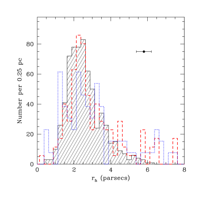
Figure 11: Histograms of globular cluster scale sizes for three galaxies. Our present results for M104 are shown as the shaded histogram; the Milky Way GCs are in shown as the dashed red histogram, and the compilation of old GCs from nearby dwarf galaxies (Georgiev et al., 2009) as the dotted blue histogram. The Milky Way and dwarf samples have been normalized to the same total population as in M104. The errorbar at upper right is the mean internal uncertainty of $\pm 0.41$ pc (see text) for our measurements.

A basic point of immediate interest is to compare the GC size distribution with the one for the “baseline” Milky Way system. However, a minor spatial bias must be kept in mind. The Sombrero GCs in our list do not cover its entire halo, whereas (in the Milky Way at least) there is a well known trend for $\langle r_{h}\rangle$ to increase systematically with $R_{gc}$ (van den Bergh al., 1991). The GCs in our data have projected galactocentric distances ranging from $R_{gc}\simeq 0.9$ kpc out to 15 kpc, with reasonably complete radial coverage to 8.5 kpc. To extract a Milky Way sample that will more closely mimic the M104 data, we take the 114 known Milky Way clusters with measured half-light radii obtained from King-model fits (Harris, 1996) and with projected Galactocentric distances $R_{gc}=(Y^{2}+Z^{2})^{1/2}<12$ kpc. Here $(Y,Z)$ are the distance components projected on the sky parallel to and perpendicular to the Galactic plane. In Figure 11 the distribution for the 114 selected Milky Way clusters is shown as the dashed red histogram. The median is at $r_{h}(MW)=2.61\pm 0.10$ pc, and to first order, the two distributions are strikingly similar. The intrinsic spread of cluster sizes around the peak is characteristically $\simeq\pm 1$ pc rms, and very few clusters exist with physical scale sizes smaller than about 1.0 pc. The slightly broader width of the central peak for M104 is likely to be due in part to the instrumental broadening of $\pm 0.4$ pc. (However, it should also be noted that the Milky Way data come from a somewhat heterogeneous collection of starcount and surface brightness data obtained in many programs for clusters at very different distances from the Sun).

Another dataset making an interesting comparison is the recently measured set of old GCs in several dwarf galaxies, from Georgiev et al. (2009). On average these small galaxies are at similar distances to M104, and their profiles were measured from HST/ACS images with ISHAPE+K62 profile fits. Georgiev et al. (2009) give data for 83 objects regarded to be classically “old”, luminous GCs. Of these, 42 clusters come from dIrr galaxies, 31 from dSph and dE systems, and 12 from Sm galaxies. The size distribution of these is plotted in Figure 11 as the blue dotted histogram. The median of this dwarf-galaxy sample is at $r_{h}=2.87\pm 0.19$ pc.

Although the medians or the peak points of these three samples are not strongly different, a potentially more important test is the total shape of the whole distribution. A standard Kolmogorov-Smirnov two-sample test shows that the M104 and Milky Way GCs are significantly different at the 97% level, whereas the M104 and dwarf samples are different at more than 99% confidence (the Milky Way and dwarf samples are not significantly different from each other). The key difference among these histograms is the relative number of “extended” clusters with $r_{h}\ga 5$ pc, i.e. the ones more than twice the median size. Our initial selection of GC candidates in M104 did not rely on object scale size except for rejection of small, starlike objects (see Paper I), so the sample should not be biased against GCs in the range $r_{h}\sim 5-10$ pc or even larger. Nevertheless, even a few more objects added to the high-end tail of the distribution would noticeably reduce the statistical difference between the Milky Way and M104, so for the present, we regard these comparisons as only indicative. Perhaps a more important conclusion is that if we use only the clusters smaller than 5 pc, there are no significant differences among these three samples.

Extended clusters would clearly find it easier to survive in the gentler tidal environment of smaller galaxies, or in the outer-halo regions of large galaxies. If we take the comparisons in Figure 9 at face value, M104 – a massive, bulge-dominated Sa galaxy – has very few such extended GCs compared with the other two samples. Possible interpretations that immediately suggest themselves are either that M104 did not acquire most of its globular cluster population by accretion of small satellites; or that any extended clusters that might have been accreted this way have already been tidally destroyed. A survey of the outer parts of M104’s halo would provide much clearer evidence to discuss this argument further.

3.2 Correlations with Metallicity

Previous surveys of GCs in nearby galaxies have shown that the blue, metal-poor clusters are consistently larger on average than the red, metal-richer ones (Kundu & Whitmore, 1998; Kundu et al., 1999; Larsen et al., 2001; Jordán et al., 2005; Spitler et al., 2006; Gómez & Woodley, 2007; Harris, 2009a). These differences are at the level of only 15-20%, but in the biggest samples (e.g. Larsen et al., 2001; Jordán et al., 2005; Harris, 2009a) they are highly significant in a statistical sense, and they are found at all galactocentric distances. Harris (2009a) determines a mean size difference of $(17\pm 2)$% (blue minus red) from a sample of several thousand clusters in six supergiant ellipticals (Brightest Cluster Galaxies or BCGs).

Our observed correlation is shown in the upper panel of Figure 12. The red clusters do lie at lower sizes on average, but an unweighted linear fit to the complete dataset gives a slope $\Delta r_{h}/\Delta(B-R)=-0.245\pm 0.191$, which is not highly significant. (See also Paper I for a similar diagram.) For all blue clusters (defined here as those with $(B-R)\leq 1.30$), the median size is $r_{h}(blue)=2.47\pm 0.04$ pc, while the redder clusters ($B-R)>1.30$) have a median $r_{h}(red)=2.33\pm 0.05$ pc. The metal-poor GCs are thus 6% larger, and the difference $\Delta r_{h}=0.14\pm 0.064$ pc is significant at the $2.2\sigma$ level, a tantalizing but not conclusive offset. In Paper I, the difference between median sizes was found to be $\Delta r_{h}=0.25\pm 0.06$ pc, similar to the present value. Thus we find the same effect seen in other systems, but at a smaller amplitude.

To date, the strongest claims for metallicity-related differences in size have relied on the large GC samples from elliptical galaxies. The samples from GCs in disk galaxies are much smaller and inevitably have lower statistical significance. Notably, however, Cantiello et al. (2007) and DeGraaff et al. (2007) find that the mean size difference for the GCs in the disk galaxies NGC 5866 and 1533 is at the level of $\sim 0.1$ pc or less, quite similar to our results for M104.

Correlation of mean size with location in the halo has been proposed as an important factor in deciding what the physical cause for the metallicity/size offset actually is (Larsen & Brodie, 2003; Jordán, 2004). If the size difference versus metallicity persists at all galactocentric distances, then it is less likely to be due to a geometric projection effect (the metal-richer clusters are usually found to have a more centrally concentrated spatial distribution than the metal-poor ones, thus will be more subject to stronger tidal stripping. This effect would be much stronger on the inner-halo clusters, and not as important for the clusters of both types that are found in the outer halo). In M104, as shown in Paper I, both red and blue GC subsystems accurately follow a $r^{1/4}-$law profile,

$${\rm log}\sigma_{GC}\,=\,\alpha R_{gc}^{1/4}\,+\,\beta\,.$$

For the red GCs, using our present data over the radial region $R_{gc}<3^{\prime}$ where we have complete azimuthal coverage, we find $\alpha=-1.937\pm 0.046,\beta=3.191\pm 0.053$; while for the blue GCs, $\alpha=-1.335\pm 0.179,\beta=2.541\pm 0.205$. Thus the blue, more metal-poor subsystem is significantly more extended. According to the geometric projection hypothesis, we would then expect a significant mean size difference between blue and red in the inner regions but less so in the outer halo.

This version of the size distribution is shown in the lower panel of Figure 12, separately for the blue and red clusters. Median values for $r_{h}$ are plotted as the connected large points with errorbars, in 1-kpc bins. The GCs of both metallicity groups have scale sizes that increase gradually but consistently throughout the halo of the galaxy. The slopes of both trends are similar, so if we combine all clusters to gain statistical weight, we find a rate of increase of mean cluster size $r_{h}\sim R_{gc}^{0.17\pm 0.02}$. The effective radius of the spheroid light is $R_{eff}=1.2^{\prime}=3.14$ kpc, so the total radial range of our data reaches to an outer limit of about $4.5R_{eff}$. Not only does the radial increase affect all clusters, but the difference between red and blue remains similar (and small) at all radii. This large-scale trend may therefore provide evidence against the geometric-projection effect (Larsen & Brodie, 2003) as being the sole explanation for the size difference in this galaxy. However, a more detailed deprojection model will be needed to test this conclusion more quantitatively (Larsen & Brodie, 2003).

The only other data in the literature that cover similarly large ranges in $R_{gc}$ are for NGC 5128 (Gómez & Woodley, 2007), which reach even further to $\simeq 8R_{eff}$ but cover a smaller sample; and for the six supergiant ellipticals studied by Harris (2009a), which extend to distances $\simeq 4.5R_{eff}$. Both of these other surveys, however, indicate the same steady increase in scale size with $R_{gc}$ for clusters of both types. So do the smaller samples in the two disk galaxies mentioned above (Cantiello et al., 2007; DeGraaff et al., 2007). Harris (2009a) derives a simple power-law scaling for gE’s of $r_{h}(med)=r_{h0}(R_{gc}/R_{eff})^{0.11}$, where the zeropoints are $r_{h0}=2.53$ pc (blue) and 2.15 pc (red). These functions are shown in Figure 12(b). Clearly, they strongly resemble our current data, bracketing the median points and indicating that the M104 GCs follow a very similar trend.

The total evidence suggests that the dependence of GC scale size on metallicity is at least partly intrinsic to the clusters, and thus due to a more local cause having to do either with their formation or later internal evolution. Jordán (2004) has proposed that it is the result of stellar-evolution timescales that depend on metallicity, coupled with many internal relaxation times of dynamical evolution that would make the metal-rich clusters appear smaller.

Another possibility is simply that the metal-richer clusters benefitted from more rapid cooling and contraction while they were still gaseous protoclusters and had not yet formed most of their stars (Harris, 2009a). Still another possibility is that all clusters started out with similar sizes during their early protocluster stage, but the star formation efficiency (SFE) was a bit higher for more metal-rich gas, allowing the cluster to expand less during the gas expulsion phase (see Section 4 below). These alternatives will be difficult to compare quantitatively, but detailed models would be of great interest.

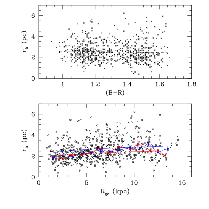
Figure 12: Upper panel: Scale sizes of M104 clusters versus $(B-R)$ color. A linear fit to the points is shown as the dashed line. Lower panel: Scale sizes for the clusters as a function of projected galactocentric distance $R_{gc}$. Blue-sequence clusters ($B-R\leq 1.3$) are plotted as crosses, red-sequence clusters ($B-R>1.3$) as open circles. Large filled circles with errorbars denote the median sizes in 1-kpc bins, separately for the blue clusters (dashed blue line) and red clusters (solid red line). The two smooth curves (blue, red) show the scaling laws $r_{h}\sim R_{gc}^{0.11}$ that have been found for globular clusters in supergiant ellipticals (Harris, 2009a).

3.3 Size versus Luminosity

The correlation of cluster scale size with luminosity is the observational version of the mass/radius relation. This form is displayed in Figure 13. Here, the individual clusters are plotted along with the median $r_{h}$ in half-magnitude bins of luminosity $M_{R}=R-(m-M)_{R}$ where our adopted apparent distance modulus is $(m-M)_{R}=29.90$. Over the range $-7\ga M_{R}\ga-10$ (corresponding approximately to the luminosity range $3\times 10^{4}$ to $6\times 10^{5}L_{\odot}$) the median size remains nearly constant, increasing more rapidly for luminosities $M_{R}\la-10$. The pattern for the GCs in the supergiant ellipticals from Harris (2009a), shown as the dashed lines in Figure 13, is the same, although these six galaxies are $\sim 5\times$ more distant than M104 and thus the GCs could not be traced to similarly faint luminosities. Here, the $(I,B-I)$ photometry used for the giant ellipticals has been converted approximately to $M_{R}$ with the assumption $R-I\simeq 0.5$.

In Figure 14, the data for M104 are plotted in comparison with two other large disk galaxies, the Milky Way and M31 (with data from Barmby et al., 2007). This form of the graph shows more clearly the trend for the most luminous GCS ($L\ga 3\times 10^{5}L_{\odot}$), extending up to the very most luminous GCs known near $10^{7}L_{\odot}$. A more extensive discussion of the possible link between massive GCs and the still more massive UCDs is made by Hasegan et al. (2005) and has been developed further in, for example, Kissler-Patig et al. (2006); Evstigneeva et al. (2008); Forbes et al. (2008). In general, UCDs have scale sizes of $\simeq 10$ pc and above, thus sit a bit higher on the $(L,r_{h})$ relation than do the GCs. The single UCD known in the M104 field is more than one magnitude brighter (Figure 10) than the top end of either the blue or red GC sequences.

A key factor distinguishing a massive GC from a UCD or nuclear cluster may be the higher mass-to-light ratio for UCDs (Mieske et al., 2008; Baumgardt & Mieske, 2008). Multiple cluster mergers are another route to forming supermassive GCs and UCD-like objects and can explain the observed upturn in the $L$ vs. $r_{h}$ correlation (e.g. Kissler-Patig et al., 2006); but it is less clear whether such mergers would also produce objects with increased $(M/L)$. It remains possible that at least some UCDs may simply be very massive GCs. This latter view is supported by Murray (2009), who develops a model for the size/mass/luminosity relation using the idea that very massive protoclusters ($\ga 10^{6}M_{\odot}$) will be optically thick to their far-IR radiation, making radiation pressure important for energy balance. The resulting increase in Jeans mass with cluster mass will yield a scaling of $M/L$ with mass that matches the trend for UCDs and the most massive GCs reasonably well.

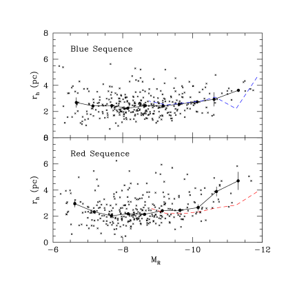
Figure 13: Upper panel: Sizes of the blue-sequence clusters ($(B-R)<1.3$) as a function of luminosity $M_{R}$. The connected solid dots with errorbars show the median $r_{h}$ in half-magnitude bins (see text). Lower panel: Sizes for the red-sequence clusters ($(B-R)>1.3$). In both panels, the mean relations for GCs in six supergiant ellipticals (Harris, 2009a) are superimposed as the dashed lines.

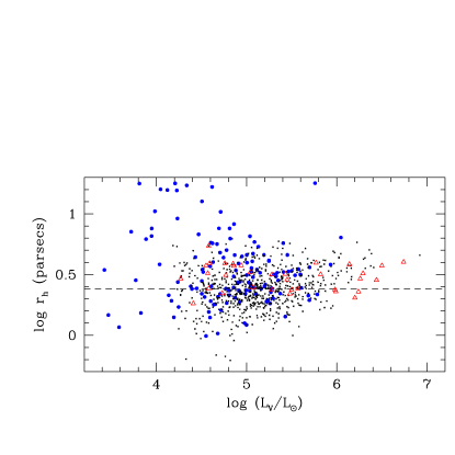
Figure 14: Scale sizes of globular clusters in three massive disk galaxies: M104 (small crosses), the Milky Way (large filled circles), and M31 (triangles). The median size of 2.4 pc is drawn in as the dashed line. Note the systematic rise in median $r_{h}$ for luminosities above log $(L_{V}/L_{\odot})$ $\ga 5.5$, as well as the scatter to high $r_{h}$ at low luminosities.

3.4 Fundamental-Plane Quantities

Recent work has established the existence of a surprisingly narrow “fundamental plane” (FP) of structural quantities for globular clusters (e.g. Djorgovski, 1995; McLaughlin, 2000; McLaughlin & van der Marel, 2005). The so-called $\kappa-$space of three orthonormal quantities $(\kappa_{1},\kappa_{2},\kappa_{3})$ is conventionally constructed from the central velocity dispersion $\sigma_{p0}$, effective radius $r_{h}$, and surface mass density $\Sigma_{h}$. For GCs in galaxies such as this one beyond the Local Group, direct velocity dispersion measurements (hence mass) are rare by comparison with photometry, and in any case require knowing the cluster core radii $r_{c}$ to convert the integrated velocity dispersion to its core value. The core radii in turn have to be estimated from $r_{h}$ and the model-fitted central concentrations $c$, which are quite uncertain for objects such as these where $r_{c}$ is far smaller than the image resolution.

Although a full discussion of the FP in all its various guises is therefore not possible, more limited versions can still be constructed. A useful quantity representing the cluster density is the surface intensity $I_{h}=L_{tot}/(2\pi r_{h}^{2})$ integrated over the half-light radius. This quantity is well enough determined to allow us to compare the M104 GC population directly with the baseline Milky Way system (see also Barmby et al., 2007, for similar data in M31 and other Local Group members). Our measurements give internal uncertainties of $\pm 0.1$ mag or better in luminosity and $\pm 0.4$ pc in radius, making (log $I_{h}$) uncertain to $\pm 0.13$. In Figure 15, $I_{Vh}$ is plotted against both cluster size and total luminosity. The analogous Milky Way data are taken from McLaughlin & van der Marel (2005). The obvious trends that $I_{h}$ is brighter for more luminous or more compact clusters are evident from the graphs, but the main conclusions to draw are that the M104 GCs match up well with both the mean positions of the Milky Way clusters and the intrinsic scatter around the fiducial scaling lines (shown in the graph). The clusters at lowest luminosities and surface brightnesses do, however, tend to have systematically larger scale sizes, dropping them below the fiducial scaling lines in both graphs. The papers listed above give more detailed discussions of these relations.

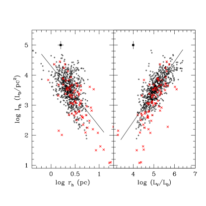
Figure 15: Surface intensity in $V$ over the half-light radius, plotted as a function of cluster scale size (left panel) and total luminosity (right panel). Small dots give the data for the M104 clusters, while the large red crosses give similar data for the Milky Way clusters (McLaughlin & van der Marel, 2005). The large square at upper left in each panel with errorbars shows the mean internal uncertainty in each datapoint. The straight lines in each graph show the nominal proportionality scalings $I_{h}\sim r_{h}^{-2}$ and $I_{h}\sim L$.

An alternate and conceptually simple formulation of the FP is in terms of the binding energy of the cluster, $E_{b}=f(c)GM^{2}/R$ (McLaughlin, 2000), where $f(c)$ represents the details of the internal mass distribution for a given cluster and $R$ is some characteristic radius. As is shown in McLaughlin (2000) and Barmby et al. (2007), for normal globular clusters the binding energy varies almost exactly as $E_{b}\sim M^{2}$ with remarkably little relative scatter, a scaling law that is basically quite different from the $E_{b}\sim M^{1.5}$ rule characterizing other structures such as giant molecular clouds or E galaxies. This form of the FP has been used for globular clusters within Local Group galaxies including the Milky Way, M31, and the Magellanic Clouds (Barmby et al., 2007). As originally defined by McLaughlin, the calculation of $E_{b}$ requires fairly precise knowledge of the King core radius and central concentration, which we do not have for M104 and other galaxies at large distances. However, McLaughlin (2000) also shows that it can be recast in terms of the effective (half-light) radius, which is much more accurately known. The major advantage of defining $E_{b}$ this way is that it allows us to extend the FP discussion to the huge cluster populations in the giant galaxies that lie in the near-field region beyond the Local Group.

An appropriate combination of the equations in McLaughlin’s paper gives

$$E_{b}\,=\,G({4\pi\over 9})^{2}{{\cal R}{\cal E}\over{\cal L}^{2}}{M^{2}\over r_{h}}\,$$ (3)

where ${\cal R},{\cal E},{\cal L}$ are all dimensionless functions of $c$ that can be calculated from the prescriptions in McLaughlin (2000). Happily, the ratio (${\cal R}{\cal E}/{\cal L}^{2}$) is nearly constant (see also McLaughlin, 2000), equalling $0.17\pm 0.02$ over the range of King $c-$values appropriate for normal GCs, so by using the half-light radius we do not need to know the central concentration precisely. A potentially more important caveat is that strictly speaking, knowing $M$ requires also knowing the cluster mass-to-light ratios. In turn, measurement of $M/L$ independently of the photometry or colors requires direct measurement of the internal velocity dispersions, which are not yet available for M104 with the exception of the bright UCD (see below). For the present purposes, we simply assume $(M/L)_{V}=2.0$ and then calculate $E_{b}$ for all the M104 clusters in our list. This fiducial $(M/L)$ is a compromise choice drawn from the recent literature for dynamically measured masses of GCs in the Milky Way, M31, and NGC 5128 (McLaughlin & van der Marel, 2005; Rejkuba et al., 2007; Strader et al., 2009; Baumgardt et al., 2009). These measurements fall in the typical range $(M/L)_{V}\simeq 1-3$, probably with real cluster-to-cluster differences depending on metallicity, luminosity, or galactocentric distance.

In Figure 16, the resulting correlation of binding energy with cluster luminosity is shown. A direct least-squares solution gives log $E_{b}/{\rm ergs}=(41.11\pm 0.07)+(1.92\pm 0.02){\rm log}L$, with a scatter of $\pm 0.16$ dex. For the Milky Way GCs McLaughlin found slopes in the range $1.8-2.2$ under various assumptions. In summary, we concur that the scaling rule $E_{b}\sim L^{2}$ provides an excellent first-order description of the data. The scatter around the line in Figure 16a is artificially small (only half as large as for the Milky Way sample) because it does not account for cluster-to-cluster differences in the $M/L$ ratio that must be present (and since $E_{b}$ varies as $L^{2}$ it is moderately sensitive to changes in $M/L$).

The UCD in the M104 field is of special interest as a possible “connector” to the GC sequence. Its position is shown in Figure 16 at upper right. The lower of the two connected points is where we would have located it if we had assumed $(M/L)_{V}=2.0$ as we did for all the GCs. The upper point uses its actual value of $(M/L)_{V}=4.36$ as directly measured from its internal velocity dispersion (Hau et al., 2009). Remarkably, its true position on the graph extends the same $E_{b}$ curve defined by the GCs accurately upward by another order of magnitude beyond the top of the GC sequence. This result, in addition to the other characteristics of the UCD measured by Hau et al. (2009), is consistent with the interpretation that this luminous, compact system is a massive GC.

The binding energy also provides a sensitive confirmation test of changes in cluster structure with environment. McLaughlin (2000) found that the residuals from $E_{b}$ vs. $L$ were a significant function of galactocentric distance in the Milky Way (see his Fig. 10), in the sense that clusters further out in the halo are less tightly bound because of their systematically larger radii. Using the results from Figure 12 and Section 3.2, we can predict that for our M104 data, $(E_{B}/L^{2})$ should vary as $R_{gc}^{(-0.17\pm 0.02)}$. The consistency test is shown in Figure 16b, where we find a net downward trend with a fitted slope of $(-0.19\pm 0.02)$ in good agreement with the prediction. For the Milky Way, McLaughlin found a slope of $-0.4\pm 0.1$ for the trend of $E_{b}/L^{2}$ versus three-dimensional Galactocentric distance, which after projection to two dimensions will decrease the slope to a level closer to our result.

Figure 16: Upper panel: Binding energy $E_{b}$ measured in ergs, plotted against cluster $V-$band luminosity in Solar units $L_{V}/L_{\odot}$. The straight line is an exact scaling law $E_{b}\sim L^{2}$. The two large starred points at upper left show the position of the UCD under two different assumptions about its M/L ratio (see text). Lower panel: Normalized binding energy $E_{b}/L^{2}$ versus projected galactocentric distance. The fitted straight line has a slope of $-0.19$ (see text).

Yet another way to represent the trend of cluster structure with galactocentric distance is as used recently by McLaughlin & Fall (2008) and Chandar et al. (2007). A characteristic mean internal mass density for each cluster can be calculated from $\rho_{h}=(M/2)\times 3/(4\pi R_{h}^{3})$ where $R_{h}\simeq(4/3)r_{h}$ is the three-dimensional half-mass radius. As above, we use $M/L=2$ to transfer from luminosity to mass. The results plotted separately for the blue (metal-poor) and red (metal-rich) clusters are shown in Figure 17. The best-fit lines through each set of points are ${\rm log}\rho_{h}(M_{\odot}pc^{-3})=(3.35\pm 0.10)-(0.51\pm 0.12){\rm log}R_{gc}$ (blue) and ${\rm log}\rho_{h}=(3.33\pm 0.10)-(0.49\pm 0.13){\rm log}R_{gc}$ (red). The scatter around both relations is $\pm 0.55$ in log $\rho_{h}$. If mean GC mass does not vary with location in the halo, as the M104 data show, then the scaling $r_{h}\sim R_{gc}^{0.17}$ (Section 3.2) would predict $\rho_{h}\sim R_{gc}^{-0.51}$, which matches what is found in the density plot. As is discussed by Chandar et al. (2007) and McLaughlin & Fall (2008), the large cluster-to-cluster scatter in density at all galactocentric distances allows the mean cluster mass to be nearly independent of $R_{gc}$ in the presence of density-dependent dynamical evolution times.

Figure 17: Calculated mean density $\rho_{h}$ plotted as a function of galactocentric distance. The metal-poor and metal-rich clusters are plotted in separate panels, with the mean relationships derived in the text shown as dashed lines.

4 Origin of the Size Distribution

Aside from minor trends with metallicity, galactocentric distance, and mass, the characteristic scale sizes and their distribution function (the SDF) in all types of galaxies are remarkably similar over an impressive range of environments. Early indications of the near-universal mean or median GC sizes on observational grounds were developed a decade ago by Kundu & Whitmore (2001) from HST/WFPC2 measurements of GC sizes in 28 elliptical galaxies, and by Larsen et al. (2001) for a larger sample of GCs in 17 ellipticals. A major step forward was taken with the work of Jordán et al. (2005), who used their database of $\sim 10^{4}$ GCs in dozens of Virgo galaxies to strongly reinforce the view that the full shape of the SDF, as well as its mean or median, is a near-universal characteristic of GCs in galaxies generally. Furthermore, the SDF has also been found to be similar over a wide range of cluster age (e.g. Barmby et al., 2006; Scheepmaker et al., 2007). Its key features are a typical median size $r_{h}\simeq 2-4$ pc, a rather sharply defined cutoff below 1 pc, and an asymmetric tail extending to larger radii. The near-universality of this distribution across all types of galaxy environments suggests to us that the conditions local to the clusters themselves, during their formation period, are an important factor in determining the observed size distribution. As Jordán et al. (2005) remark, “The form of the distribution … should serve as a useful constraint for models of GC formation … any viable picture of star formation in clusters should produce an observed size distribution that is consistent with the form of [the SDF]”.

A more well known feature of GC systems within galaxies in general is their mass (luminosity) distribution (GCLF), which is also a near-universal function relatively insensitive to host galaxy size or environment. The GCLF can be modelled as the outcome of a power-law-like initial mass function coupled with many Gyr of dynamical evolution, which preferentially removes the low-mass and low-density clusters and reduces the IMF to the peaked Schechter-like form seen today (for only a handful of the dozens of papers discussing the mass distribution function and its secular evolution, see Baumgardt & Makino, 2003; Whitmore et al., 2007; Jordán et al., 2007; McLaughlin & Fall, 2008; Gieles & Baumgardt, 2008; Kruijssen & Portegies Zwart, 2009). By contrast, the origin of the linear size distribution for GCs has received less attention. But the state of development of both observations and models is now reaching the point where some paths to understanding it are opening.

As stated above, the GC effective radius remains nearly invariant over the normal dynamical evolution of the cluster – much more so than the total mass of the clusters, which decreases by factors of 3 or more over a Hubble time as it loses stars through the slow processes of tidal stripping and evaporation. Thus $r_{h}$ gives us an unusually direct glimpse of its characteristic size much closer to its origin. However, extrapolating the current effective radius all the way back to its protocluster epoch is highly unlikely to be correct. A crucial stage in its evolution occurs just after formation, when it consists of a mixture of gas and stars in proportions determined by the star formation efficiency (SFE). Especially over its first $\sim 30$ Myr, a cluster experiences rapid mass loss due to the energy output from its massive stars, including UV radiation, supernova ejection, stellar winds, and even external dynamical heating. These effects expel the gas and drive an internal expansion of the cluster. For the extreme case of low SFE and instantaneous gas loss this stage would lead to rapid dissolution of the cluster into the field. For bound star clusters, however, both observations (Mackey & Gilmore, 2003; Bastian et al., 2008) and theory (see, e.g. Baumgardt & Kroupa, 2007, for a thorough overview) show that for plausible SFEs, the cluster expands typically by a factor of $2-5$ over this crucial initial stage. An empirical expression for the growth of core radius with age for real clusters (Bastian et al., 2008) is $r_{core}=0.6{\rm ln}\{(\tau/10^{6}y)-0.25\}$. After $\sim 10^{8}$ years, the cluster settles into its long-term phase of slower internal dynamical evolution and stellar evaporation.

In addition, the observational evidence so far (Mackey & Gilmore, 2003; Bastian et al., 2008), though admittedly still sketchy, indicates that the extremely young clusters show a smaller spread of core radii than the older ones. It is therefore tempting to see the shape of the present-day SDF (see again Figure 11) as the result of cluster-to-cluster differences in the star formation efficiency, starting from a population of protocluster cores that began with rather similar sizes. The single-peaked but slightly asymmetric shape of the size distribution is strongly reminiscent of a normal probability distribution that has passed through a nonlinear transformation. In this case, the transformation is the conversion of a given SFE to a radial expansion factor.

In this view, the peak frequency at $r_{h}\simeq 2-3$ pc would simply represent protoclusters which experienced the most common (i.e. most probable) SFE. Smaller values of the initial SFE would lead to clusters with a larger present-day size, and the very largest clusters would be ones with SFEs not much above the minimum level required to remain bound. At the opposite extreme, protoclusters with unusually high SFE would suffer only very small expansion and end up at the minimum observed size of $\sim 1$ pc. Said differently, the “rise point” of the SDF at $r_{h}\simeq 1$ pc should therefore be close to the typical initial size of the protoclusters.

The actual mean SFE within any one protocluster should in principle be determined by several factors (e.g. local temperature, pressure, turbulence, degree of initial mass segregation), and thus could vary stochastically from one core to another. However, the mean SFE is expected (cf. Lada & Lada, 2003) to be near 30% for dense star-forming regions that will give rise to massive clusters. This mean SFE already permits an independent estimate of the amount of radial expansion to be expected, from analytical energy arguments: in the limit of slow, adiabatic expansion during gas expulsion, the product (cluster mass $\times$ radius) stays constant (Hills, 1980), which yields an expansion factor of $(SFE)^{-1}\simeq 3.3$. This suggests in turn that the initial sizes of the protoclusters should be near $\sim 0.8$ pc to produce a present-day median around 2.5 pc, consistent with the observations cited above.

The models by Baumgardt & Kroupa (2007) (BK07) allow us to explore some simple simulations of the SDF a bit further along the lines outlined above. BK07 use three critical factors determining the final expansion ratio $ER=r_{h}(final)/r_{h}(initial)$: (a) the SFE in the protocluster, (b) the initial cluster size relative to its tidal radius $(r_{h}/r_{t})$, and (c) the ratio of the “mass loss time” $\tau_{M}$ over which gas is expelled relative to the internal crossing time $t_{C}$. As argued above, we expect the protocluster core to be typically $\sim 0.5-1$ pc in size. This level is far smaller than the typical tidal radius of $\ga 50$ pc for a massive globular cluster, so for our purposes we assume a small $(r_{h}/r_{t})<0.03$ (see Figure 4 of BK07). In addition, the very large amount of dense gas present in the core during star formation will be capable of absorbing and thermalizing the SNe ejecta and stellar winds, preventing instantaneous mass loss (see also Bailin & Harris, 2009). In these massive protoclusters as well, the crossing time $t_{C}\sim 10^{5}$ y is less than the gas expulsion time (Goodwin, 1997; Baumgardt & Mieske, 2008). We therefore use the BK07 models for the two representative cases $\tau_{M}=t_{C}$ (moderately rapid but not instant gas expulsion) and $\tau_{M}=10t_{C}$ (slow, near-adiabatic gas expulsion).

It should be noted that we do not expect these setup arguments to carry over identically for low-mass clusters. For these, the smaller tidal radius will mean more rapid escape of stars during the expansion phase as well as more rapid expulsion of gas (Baumgardt & Mieske, 2008), both of which put the early evolution into a different regime of the model parameter space. At masses well below the normal GC range, a far higher fraction of the protoclusters will not survive this initial mass-loss stage.

With these assumptions about the tidal limit and mass loss time, the dispersion in the resulting cluster sizes starting from a fixed initial core size will be due simply to a dispersion in the SFE’s from one cluster to another. To model the SFE in a simple way, we assume that it follows a Gaussian distribution with a mean of $E_{0}$ and a standard deviation of $\sigma_{E}$. In general, this approach resembles the grid of simulations by Baumgardt & Mieske (2008) drawing from the same models. However, their work was directed towards exploring the trends of mean cluster mass and radius as functions of galactocentric distance. Here, we concentrate on attempting to reproduce the detailed shape of the SDF itself.

Using the BK07 model grid, we find that the relation between the formation efficiency and the expansion ratio $ER$ can be well approximated by $ER\simeq 0.55(SFE)^{-1.6}$ for the rapid case $\tau_{M}=t_{C}$. As already noted above (cf. Hills, 1980), $ER=(SFE)^{-1}$ for the slow-expulsion case $\tau_{M}=10t_{C}$. We then run Monte Carlo realizations with these assumptions, and vary $E_{0},\sigma_{E}$, and the initial cluster size $r_{h}(init)$ to find simulations that match the real distributions. A final bit of input is to convert the initial cluster radius $r_{h}$ (three-dimensional) to the projected $r_{h}$ that we observe with the correction factor $r_{h}(proj)=0.73r_{h}(3D)$.

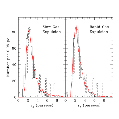
Figure 18: The scale size distributions for the globular clusters in M104 (solid histogram) and the Milky Way (dashed histogram), repeated from Figure 11. In the left panel, the solid red line shows a simulated $r_{h}$ distribution for model clusters with slow gas expulsion and a range of star formation efficiencies averaging $SFE=0.28,\sigma_{E}=\pm 0.11$ as described in the text. In the right panel the red line shows a simulated distribution for rapid gas loss and a mean $SFE=0.30,\sigma_{E}=0.07$.

Figure 18 shows the results of two sample runs, matched to the data shown previously for M104 and the Milky Way. Each simulation is the result of generating $10^{4}$ clusters at random following the prescriptions described above. The left panel shows the “slow expulsion” case for the parametric values $E_{0}=0.28$, $\sigma_{E}=0.11$, and $r_{h}(init)=1.0$ pc. The right panel shows the “rapid expulsion” case for $E_{0}=0.30$, $\sigma_{E}=0.07$, and $r_{h}(init)=0.9$ pc. Both the simulations and the Milky Way distribution have been normalized to the total population of the M104 system. Both models match the real data encouragingly well. The three important features are the rapid ramp-up in numbers of clusters starting at $r_{h}\simeq 1$ pc; the moderately broad peak near 2.5 pc; and the long but low-amplitude tail extending to much larger radii.

A limitation of the present discussion is obviously that we have not properly included the long-term effects of dynamical evolution on the SDF. These effects would progressively trim the SDF that emerged shortly after the early gas-loss phase, gradually removing low-mass or very low-density objects. For this reason, our SDF models which predict a few more clusters at larger radii than in the present-day data are probably not a cause for serious worry, because these large-radius, low-density clusters are among the ones that would preferentially get destroyed by dynamical evolution over the subsequent Hubble time. The high$-r_{h}$ tail predicted by the models should therefore be only an upper limit to the present-day distribution.

Da Costa et al. (2009) have collected the recent observations for the SDF particularly in dwarf galaxies, and develop intriguing evidence that the SDF in total may be bimodal. The “normal” mode peaked at $r_{h}\simeq 2.5-3.0$ pc is the more well populated of the two, but there is a second mode peaked near $r_{h}\simeq 8$ pc. There are no obvious observational selection effects that would bias discoveries (or size measurements) against cluster in the intermediate-size range around 5 pc between the two modes, so the reality of the bimodality must be taken seriously. Da Costa et al. propose that these may belong to a second mode of cluster formation more prevalent in the weaker potential wells of the dwarfs.

Figure 19 shows a match of our model to the old-GC sample compiled from several dwarf galaxies by Georgiev et al. (2009) described above, where we attempt to match the bimodal distribution noted by Da Costa et al. The normal mode (solid line) is the fast-expulsion model for $E_{0}=0.32$, $\sigma_{E}=0.08$, and $r_{h}(init)=1.15$ pc, while the “extended” upper mode (dashed line) assumes $E_{0}=0.30$, $\sigma_{E}=0.03$, and $r_{h}(init)=2.4$ pc. Reproducing the upper mode requires a distinctly larger initial protocluster radius, though interestingly, it needs to be larger by only a factor of two. The formal value of $\sigma_{E}$ is quite a bit lower than for the normal mode, but once again it is less clear how significant this is, because clusters that ended up with very large radii $r_{h}\ga 15$ pc might not have survived except (as also discussed by Da Costa et al.) under the most favorable circumstances. Minor variations around these combinations of parameters can be found that give similar fits, and the present discussion should be taken only as illustrative.

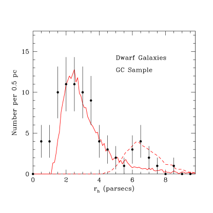
Figure 19: The scale size distributions for the sample of globular clusters in dwarf galaxies, from Georgiev et al. (2009) as described in the text. The solid (red) line shows a simulated model distribution for the rapid gas expulsion case with $E_{0}=0.32$, $\sigma_{E}=0.08$, $r_{h}(init)=1.15$ pc. The dashed line shows a comparable simulation but now with $E_{0}=0.30$, $\sigma_{E}=0.03$, and $r_{h}(init)=2.4$ pc.

Lastly, Figure 20 shows the sensitivity of the model SDF to changes in both the basic SFE and the initial core size $r_{h}(init)$. The same model fit as in Figure 18b for relatively rapid expulsion (solid line) is shown ($E_{0}=0.30,\sigma_{E}=0.07,r_{h}(init)=0.9$) along with the Milky Way cluster data. The dashed and dotted lines in the left panel show the same model but now with only the mean SFE changed ($E_{0}=0.35,0.25$). The right panel shows models for changes in only the initial radius ($r_{h}(init)=0.7,1.1$). These four outlying models clearly fail to match the data. The implications are that the average starting conditions are constrained to rather narrow ranges, $\pm 0.05$ or less in $E_{0}$ and $\pm 0.1$ pc or less in $r_{h}(init)$. To a large extent, variations in $r_{h}(init)$ can be traded off with variations in $E_{0}$ to produce the final range of observed sizes.

In rougher terms, the appropriate ranges for the initial conditions can be understood physically as follows. If $E_{0}$ falls below $0.20-0.25$, then very few clusters survive the gas expulsion phase at all. At the opposite end, values of $E_{0}$ higher than about 0.4 mean that most clusters experience too little expansion to reproduce the peak at 2.5 pc or to fill up the high$-r_{h}$ tail. For the initial size, values of $r_{h}(init)$ bigger than $\sim 1$ pc or less than $\sim 0.7$ pc drive the present-day peak well above or below the characteristic 2.5-pc level that we need, and also fail to match the observed absolute range in the SDF. Finally, the third fitting parameter $\sigma_{E}$ is essentially used to fine-tune the SDF peak and dispersion, once $E_{0}$ and $r_{h}(init)$ have been put into the right range.

These sample realizations are undoubtedly oversimplified, and do not by any means represent a thorough exploration of the parameter space of the models. This approach also ignores other potentially interesting effects such as external interactions with other clouds; mergers of young clusters; clumpiness and substructure within a protocluster; or primordial mass segregation. All of these could affect the early structural evolution (e.g. Scheepmaker et al., 2007; Baumgardt et al., 2008; Marks et al., 2008).

Our main point, however, is that it seems possible to understand the key features of the globular cluster size distribution with a relatively simple set of assumptions, and with quite plausible fiducial values for the range of star formation efficiencies and initial protocluster sizes. Various arguments in the literature already favor a mean SFE of around 30 percent for star clusters (e.g. Lada & Lada, 2003) and an initial size less than 1 pc (Bastian et al., 2008). However, there are far fewer avenues to quantitative estimates for the range of SFE’s and initial scale sizes that typified the formation regions of massive star clusters. The detailed shape of the present-day size distribution appears to be one such method.

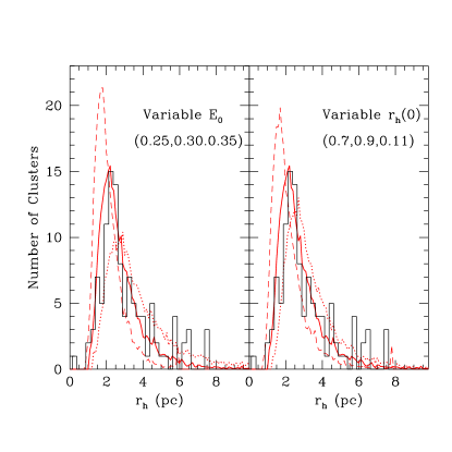
Figure 20: Left panel: The solid histogram shows the size distributions for the Milky Way globular clusters. The red solid line is the “best-fit” model for rapid gas expulsion ($E_{0}=0.30,\sigma_{E}=0.07,r_{h}(init)=0.9$ pc) while the dashed and dotted lines show models for $E_{0}=0.35$ and $0.25$. Right panel: Same as in previous panel, but here the red dashed and dotted lines show models for $r_{h}(0)=r_{h}(init)=0.7$ and 1.1 pc.

5 Bimodality and the Mass/Metallicity Relation

M104 was one of the first galaxies in which the intriguing correlation between mean luminosity and color along the blue sequence was found (Paper I). This trend acts in the sense that the most luminous clusters become slightly but progressively more metal-rich, and thus corresponds to a mass/metallicity relation (MMR). The original discovery papers used samples of data from large elliptical galaxies (Harris et al., 2006; Strader et al., 2006; Mieske et al., 2006), but the M104 data indicated that it might extend to disk systems as well. The first round of papers gave different results for the detailed shape of the MMR, but more recent data analysis and discussions (Harris, 2009a, b; Peng et al., 2009; Cockcroft et al., 2009) indicate more of a consensus emerging around the view that the blue sequence is nearly vertical for lower luminosities ($L\la 5\times 10^{5}L_{\odot}$) but gradually slants more toward the red going up to higher luminosities. Equally intriguingly, no such MMR seems to affect the red sequence, which keeps the same mean metallicity at all luminosities.

The most effective physical interpretation so far is based on some form of self-enrichment during a cluster’s formation stage (Strader & Smith, 2008; Bailin & Harris, 2009). A protocluster of mass $\ga 10^{7}M_{\odot}$ or more, within a core of $\sim 1$ pc, will be able to hold back enough of its first round of SN-enriched material to enrich the still-forming low-mass stars, thus giving the entire cluster a higher mean metallicity than the pre-enriched level it started with. This extra self-enrichment will be much less noticeable along the red sequence because its protocluster gas is an order of magnitude higher in heavy-element abundance than the blue sequence.

We have used our new photometry of the M104 clusters to re-investigate the existence of an MMR within this massive disk galaxy. As noted above, all the $BVR$ total magnitudes are individually corrected for the scale sizes of the clusters and thus are free of any aperture-size or PSF-fitting effects that might depend on luminosity. The first test is to measure any correlation of mean color with luminosity along both sequences. To do this, we use the $(B-R)$ data as the most metallicity-sensitive of the three possible color indices we could define, and then divide the data into half-magnitude bins by $R$ magnitude. The color distribution is then put into the fitting routine RMIX (Wehner et al., 2008; Harris, 2009a) and the best-fit bimodal Gaussian distributions are found in each independent interval. In this way, we do not assume any particular form for the MMR along either sequence.

Table 2: Bimodal Fits to the Color Distributions

$R$ Range	$\langle R\rangle$	n	$\mu_{1}$	$\mu_{2}$	Blue Fraction
22.5-23.5	22.92	95	$1.118\pm 0.013$	$1.479\pm 0.015$	$0.434\pm 0.054$
22.0-22.5	22.21	103	$1.121\pm 0.029$	$1.448\pm 0.031$	$0.463\pm 0.102$
21.5-22.0	21.74	131	$1.162\pm 0.016$	$1.452\pm 0.022$	$0.489\pm 0.070$
21.0-21.5	21.29	116	$1.169\pm 0.022$	$1.449\pm 0.035$	$0.507\pm 0.104$
20.5-21.0	20.77	82	$1.175\pm 0.013$	$1.494\pm 0.017$	$0.549\pm 0.059$
20.0-20.5	20.28	55	$1.214\pm 0.017$	$1.470\pm 0.027$	$0.548\pm 0.087$
19.5-20.0	19.78	36	$1.178\pm 0.018$	$1.499\pm 0.028$	$0.561\pm 0.088$
19.0-19.5	19.32	17	$1.258\pm 0.032$	$1.518\pm 0.047$	$0.522\pm 0.153$
18.0-19.0	18.68	16	$1.278\pm 0.022$	$1.520\pm 0.061$	$0.733\pm 0.124$

Figure 21: Histogram of $(B-R)$ colors for the M104 globular clusters in the magnitude interval $20.5<R\leq 23.5$ (solid points with errorbars). The solid curve shows the best-fit bimodal Gaussian, with the two individual modes shown as dashed lines.

The mean points derived from these objective fits are listed in Table 2 and plotted in Figure 22. In principle, RMIX can solve for five free parameters: the mean colors $\mu_{1},\mu_{2}$ of the blue and red modes; their Gaussian dispersions $\sigma_{1},\sigma_{2}$; and the proportion $p_{1}$ (or $p_{2}=1-p_{1}$) that the blue (red) mode makes up of the total population. In practice, if the number of datapoints in the bin is less than about 50, the solutions need to be partially constrained for convergence; here, we choose in such cases to fix the dispersions $\sigma_{1,2}$ because these do not change noticeably along the sequence and we are primarily interested in tracing the mean colors themselves. By using the total data over $20.5<R<22.0$ we find $\langle\sigma_{1}\rangle=0.070\pm 0.006$ and $\langle\sigma_{2}\rangle=0.096\pm 0.010$. The color distribution in $(B-R)$ for this galaxy defines a remarkably clear bimodal histogram (Figure 21), and the double-Gaussian model provides an accurate fit.

As can be seen from Table 2, the blue and red clusters make up nearly equal proportions of the total population; the $p_{1}(blue)$ ratio increases steadily toward higher luminosity and the blue sequence reaches a bit higher at the top end. As expected from both the previous literature and the self-enrichment model, the red sequence does not show a significant change in mean color with luminosity (that is, it has a “zero” MMR). By contrast, the blue sequence shows a clear slope toward the red that is nearly linear in form. An unweighted linear fit to the mean points in Table 2 gives a highly significant slope $\Delta(B-R)/\Delta M_{R}=-0.037\pm 0.005$, almost identical with what was derived in Paper I. In terms of heavy-element abundance $Z$ this slope corresponds to a scaling $Z\sim L^{0.29\pm 0.04}$ (see below).

The slope of the linear fit becomes progressively less significant as the higher-luminosity bins are removed. For example, a direct fit of $(B-R)$ versus $R$ for the clusters with $M_{R}>-8$ and $(B-R)_{0}<1.20$ gives $\Delta(B-R)/\Delta M_{R}=-0.013\pm 0.014$. Thus we cannot rule out the possibility that the blue sequence may become more nearly vertical at lower luminosities. Nevertheless, we confirm the basic trend found in Paper I that the blue sequence does show an MMR. In addition, the metallicity scaling agrees extremely well with the mean slopes $Z\sim L^{0.3}$ found for several giant E galaxies in the recent studies by Harris (2009a), Harris (2009b), and Cockcroft et al. (2009), and gives some additional support to the idea that the MMR may be a near-“universal” phenomenon which requires a broad-based physical explanation independent of galaxy type.

Figure 22: Left panel: Color-magnitude data for the globular clusters in M104, from Figure 10 and transformed to absolute magnitude $M_{R}$ versus intrinsic color $(B-R)_{0}$. Along each sequence the mean points in half-magnitude intervals (Table 2) are plotted as the connected large dots. The large star at top marks the UCD. Right panel: A simulated set of data from a bimodal metallicity distribution, as described in the text. At high mass the clusters are noticeably affected by self-enrichment.

As a more direct comparison between theory and data, we show in Figure 22b the same mean points from the color-magnitude diagram, but now superimposed on a simulation drawn from the Bailin & Harris (2009) theory. In this model, the clusters are assumed to form from dense protoclusters of mass $M_{0}$, initial size $r_{0}$, and with star formation efficiency $E_{0}$. The protocluster gas has a pre-enriched metallicity level [m/H]₀, which is then enriched further by some fraction of the first SNe that go off in the emerging cluster. After its formation stage, the early gas expulsion leaves the cluster with a mass $M_{0}\times E_{0}$. Then to take account of the longer-term dynamical mass loss that follows, we use the conventional expression for a roughly constant mass loss rate applying to two-body relaxation in tidally limited clusters, $M(t)\simeq M_{0}-\mu_{ev}t$ (e.g. Baumgardt & Makino, 2003; McLaughlin & Fall, 2008). The actual mass loss rate $\mu_{ev}$ is expected to be a function of cluster density; for example, McLaughlin & Fall (2008) derive $\mu_{ev}=1100\rho_{h}^{1/2}$ $M_{\odot}$ Gyr^-1 where $\rho_{h}$ is in $M_{\odot}$ pc^-3. The empirical evidence shows that the characteristic density $\rho_{h}$ in turn increases systematically with mass roughly as $\rho_{h}\sim M$, though it shows large cluster-to-cluster scatter (see Figure 1a of McLaughlin and Fall, for example). A fully detailed simulation of these effects is beyond the scope of our discussion, but as a first-order representation of the mean trend, we use $\mu_{ev}\simeq 5000(M/10^{5}M_{\odot})^{1/2}$ $M_{\odot}$ Gyr^-1, which reasonably reproduces the mass loss rates in the N-body simulations by Baumgardt & Makino (2003) and more recent work of Kruijssen & Portegies Zwart (2009) and Hurley (private communication). To set the other parameters in the enrichment model, for all clusters we use $E_{0}=0.3,r_{0}=1$ pc (Section 4 above). We also use a supernova conversion efficiency $f_{SN}=0.3$ (that is, 30% of the SNe in the cluster formation sequence happen soon enough in the burst to help enrich the remaining gas).

The initial (pre-enriched) values for the metallicities of each sequence are chosen to match the two observed sequences, at $(B-R)_{0}=1.09$ (blue) and 1.39 (red). (Note here that these are the dereddened colors, which we use for the simulations and plot in Figure 22. The data in Table 2 are the directly observed colors with no reddening removed.) Transformation between metallicity and color is determined by $(B-R)_{0}\,=\,0.27{\rm[Fe/H]}+1.52$ (Barmby et al., 2000; Cantiello et al., 2007). We assume a mass-to-light ratio $(M/L)_{R}=2$ and convert to absolute magnitude with $M_{R}=4.29-2.5{\rm log}(L/L_{\odot})$. Finally, the sequences are assumed to have intrinsic dispersions in metallicity of $\pm 0.26$ dex (blue) and 0.36 dex (red).

With this input, we then construct Monte Carlo realizations of the entire GCS, a typical example of which is shown in Figure 22b. The initial mass distribution is drawn randomly from a simple power law form $dN/dM_{0}\sim M_{0}^{-2}$, and the total number of simulated clusters is chosen to match the observed numbers in M104 for $M_{R}\la-8$. Because of our overly simplistic initial mass function for the input clusters, the simulation overestimates the numbers both at very high and low luminosity; however, the important feature is the matchup in the mean position of each sequence.

We find that the self-enrichment model can reproduce the red and blue sequences basically well. On the blue sequence, the “cut-on” point where self-enrichment starts clearly to dominate over the pre-enriched level is at $M_{R}\simeq-10$ ($M\simeq 10^{6}M_{\odot}$), above which the sequence starts to slant more strongly to the red. At very high luminosity, both sequences converge towards an enrichment level [m/H] $\simeq-0.4$ or $(B-R)_{0}\simeq 1.4$, very near where the M104 UCD sits in the color-magnitude diagram.

A second-order concern is the discrepancy between model and data for the low-luminosity range $M_{R}>-8$. The real clusters in this range appear to be slightly more enriched (redder) than their simulated counterparts. The model, as it stands, firmly predicts a “zero MMR” at present-day masses below about $10^{5}M_{\odot}$; even in their more massive protocluster state, such clusters are simply not massive or dense enough to hold back significant amounts of the enriched SNe ejecta. In other words, the model provides a good quantitative explanation for the MMR at the upper end of the sequences, but cannot explain any MMR that might continue to lower masses. Thus if the MMR genuinely extends to lower luminosities (which we take our data to hint at, though not conclusively), either the model is incomplete or another explanation must exist.

The main free parameters in the model are the SFE $E_{0}$, initial size $r_{0}$, and SN conversion efficiency $f_{SN}$. In principle, we could adjust these to force the blue cut-on point to lower luminosities: for example, making the SFE mass-dependent such that $E_{0}$ is higher at lower masses, or making $r_{0}$ smaller for the lower-mass clusters, would raise the resulting enrichment at lower mass. We could also make $f_{SN}$ arbitrarily higher only for the lower-mass clusters, but it is not clear what might produce such a counterintuitive effect. Decreasing $r_{0}$ to 0.5 pc or increasing $f_{SN}$ to 1.0 have about the same effect of lowering the cut-on point by less than a factor of two, and combining both effects would reduce it to $4\times 10^{5}M_{\odot}$. However, changes of this type away from their nominal values of $E_{0}=0.3$ and $r_{0}\simeq 1$ pc would dramatically alter the resulting SDF and are thus ruled out by the analysis presented in Section 4 above. In addition, they would increase the self-enrichment at higher luminosity even further, and destroy the matchup with the real data for $M>10^{6}M_{\odot}$.

For the present time, we see no reason to discard the basic approach of the self-enrichment model, which is quite effective at matching the central features of the MMR particularly for the high-luminosity clusters. The present study should be viewed as only an indication that further interesting tests may rely on the detailed features of the GC metallicity distribution over the entire run of luminosities.

6 Summary

In this study we have used a mosaic of HST/ACS images of the Sombrero galaxy (M104) to make new measurements of its large globular cluster population. We obtain new $BVR$ photometry and effective-radius measurements for a total of 652 clusters. Our findings include the following:

(1) The individual cluster profiles have been fitted with King and Wilson dynamical models to derive their effective (half-light) radii $r_{h}$. A series of tests of the data with different fitting models and different definitions of the stellar point-spread function show that the internal precision of the half-light radii is typically $\pm 0.4$ pc.

(2) The distribution function of the effective radii (SDF) has a peak near $r_{h}=2.4$ pc and an asymmetric tail to larger radii, which to first order is remarkably similar to the SDFs found for other galaxies, including the Milky Way, giant E galaxies, and several kinds of dwarf galaxies. We find second-order trends with cluster metallicity and spatial location (the clusters are slighter bigger on average at lower metallicity, or larger galactocentric distance). Both of these trends also resemble what has been found in other galaxies in several other recent studies. However, closer comparisons with other data in the literature show that the metallicity-based size difference may not be as large for GCs in disk galaxies as in E galaxies.

(3) The M104 GCs define very much the same regions in the structural Fundamental Plane as in other, more well resolved systems including the standard Milky Way. We use the half-light surface brightness $I_{V,h}$ and binding energy $E_{b}$ to demonstrate that clusters become preferentially more extended at larger galactocentric distances or low luminosities. As long as the cluster half-light radii can be measured accurately, these quantities can be used in still more distant systems such as the giant ellipticals in Virgo and elsewhere.

(4) We have explored a simple framework for the physical origin of the globular cluster scale-size distribution. We assume that GCs start as dense, massive protoclusters which form stars at a certain efficiency and then expand to radii near their present-day sizes during a rapid initial stage of mass loss and residual gas expulsion. Using models by Baumgardt & Kroupa (2007), we find that the observed SDF can be successfully and closely matched if we assume that (a) the protoclusters began with scale sizes $\simeq 0.8-0.9$ pc; (b) the mean star formation efficiency was $\simeq 0.30$ but with stochastic cluster-to-cluster variations on the order of $\pm 0.08-0.15$; and (c) the gas expulsion time was at least as long as the internal crossing time.

(5) The color-magnitude distribution for the GCs shows a clearly defined, classic bimodal form with nearly equal numbers of metal-poor and metal-rich clusters. Detailed bimodal fitting of the $(B-R)$ colors shows that the blue, metal-poor sequence exhibits a well determined mass/metallicity relation (MMR), becoming slightly but steadily redder towards higher luminosity. The red sequence is vertical over the entire luminosity range. Detailed comparisons with the self-enrichment model of Bailin & Harris (2009) show that a close first-order match to the data can be obtained with the same choice of star formation efficiency and protocluster size that are required to successfully model the SDF. However, a potential problem for the model may lie in whether or not the MMR extends further down the blue sequence below the point where self-enrichment can be expected to work. This will be an intriguing area for future work.

References

- Aarseth & Heggie (1998) Aarseth, S. J., & Heggie, D. C. 1998, MNRAS, 297, 794
- Bailin & Harris (2009) Bailin, J., & Harris, W.E. 2009, ApJ, 695, 1082.
- Barmby et al. (2000) Barmby, P., Huchra, J.P., Brodie, J.P., Forbes, D.A., Schroder, L.L., & Grillmair, C.J. 2000, AJ 119, 727.
- Barmby et al. (2006) Barmby, P., Kuntz, K. D., Huchra, J. P., & Brodie, J. P. 2006, AJ, 132, 883.
- Barmby et al. (2007) Barmby, P., McLaughlin, D. E., Harris, W. E., Harris, G. L. H., & Forbes, D. A. 2007, AJ, 133, 2764
- Bastian et al. (2008) Bastian, N., Gieles, M., Goodwin, S.P., Trancho, G., Smith, L.J., Konstantopoulos, I., & Efremov, Y. 2008, MNRAS, 389, 223.
- Baumgardt et al. (2009) Baumgardt, H., Côté, P., Hilker, M., Rejkuba, M., Mieske, S., Djorgovski, S.G., & Stetson, P.
- Baumgardt et al. (2002) Baumgardt, H., Hut, P., & Heggie, D. C. 2002, MNRAS, 336, 1069
- Baumgardt & Kroupa (2007) Baumgardt, H., & Kroupa, P. 2007, MNRAS, 380, 1589.
- Baumgardt & Makino (2003) Baumgardt, H., & Makino, J. 2003, MNRAS, 340, 227
- Baumgardt et al. (2008) Baumgardt, H., De Marchi, G., & Kroupa, P. 2008, ApJ, 685, 247.
- Baumgardt & Mieske (2008) Baumgardt, H., & Mieske, S. 2008, MNRAS, 391, 942.
- Brodie & Strader (2006) Brodie, J. P., & Strader, J. 2006, ARAA, 44, 193
- Cantiello et al. (2007) Cantiello, M., Blakeslee, J. P., & Raimondo, G. 2007, ApJ, 668, 209
- Chandar et al. (2007) Chandar, R., Fall, S. M., & McLaughlin, D. E. 2007, ApJ, 668, L119.
- Chandar et al. (2006) Chandar, R., Fall, S. M., & Whitmore, B. C., 2006, ApJ, 650L, 111
- Chandar et al. (2004) Chandar, R., Whitmore, B. C., & Lee, M. G., 2004, ApJ, 611, 220
- Cockcroft et al. (2009) Cockcroft, R., Harris, W.E., Wehner, E.M.H, Whitmore, B.C., & Rothberg, B. 2009, AJ, in press (arXiv:0906:2008)
- Da Costa et al. (2009) Da Costa, G.S., Grebel, E.K., REjkuba, M., & Sharina, M.E. 2009, AJ, 137, 4361.
- DeGraaff et al. (2007) DeGraaff, R.B., Blakeslee, J.P., Meurer, G.R., & Putman, M.E. 2007, ApJ, 671, 1624.
- Djorgovski (1995) Djorgovski, S. 1995, ApJ, 438, L29
- Evstigneeva et al. (2008) Evstigneeva, E. A., Drinkwater, M. J., Peng, C. Y., Hilker, M., DePropris, R., Jones, J. B., Phillips, S., Gregg, M. D., & Karick, A. M. 2007, AJ, 136, 461
- Forbes et al. (2008) Forbes, D.A., Lasky, P., Graham, A.W., & Spitler, L. 2008, MNRAS, 389, 1924
- Georgiev et al. (2009) Georgiev, I. Y., Puzia, T. H., Hilker, M., & Goudfrooij, P. 2009, MNRAS, 392, 879
- Gieles & Baumgardt (2008) Gieles, M., & Baumgardt, H. 2008, MNRAS 389, L28.
- Gómez & Woodley (2007) Gómez, M., & Woodley, K. A. 2007, ApJ, 670, L105
- Goodwin (1997) Goodwin, S. P. 1997, MNRAS,284, 785.
- Goudfrooij et al. (2007) Goudfrooij P., Strader J., Brenneman L., Kissler-Patig M., Minniti D., & Huizinga E., 2003, MNRAS, 343, 665
- Harris (1996) Harris, W.E. 1996, AJ, 112, 1487
- Harris (2001) Harris, W.E. 2001, in Star Clusters, Saas-Fee Advanced Course 28, Swiss Society for Astronomy and Astrophysics, ed. L. Labhardt and B. Binggeli (Springer)
- Harris (2009a) Harris, W.E. 2009a, ApJ, 699, 254
- Harris (2009b) Harris, W.E. 2009b, ApJ, in press (arXiv:0908.1120).
- Harris & Pudritz (1994) Harris, W. E., & Pudritz, R. E. 1994, ApJ, 429, 177
- Harris et al. (2006) Harris, W.E., Whitmore, B.C., Karakla, D., Okon, W., Baum, W.A., Hanes, D.A., & Kavelaars, J.J. 2006, ApJ, 636, 90
- Hau et al. (2009) Hau, G. K. T., Spitler, L. R., Forbes, D. A., Proctor, R. N., Strader, J., Mendel, J. T., Brodie, J. P., & Harris, W. E. 2009, MNRAS, 394, 97
- Hasegan et al. (2005) Hasegan, M. et al. 2005, ApJ, 627, 203
- Hills (1980) Hills, J.G. 1980, ApJ, 235, 986.
- Hoaglin et al. (1983) Hoaglin, D.C., Mosteller, F., & Tukey, J.W. 1983, Understanding Robust and Exploratory Data Analysis (John Wiley & Sons), pp. 404 – 414.
- Hodge (1962) Hodge, P. W. 1962, PASP, 74, 248
- Jordán (2004) Jordán, A. 2004, ApJ, 613, L117
- Jordán et al. (2005) Jordán, A. et al. 2005, ApJ, 634, 102
- Jordán et al. (2007) Jordán, A., McLaughlin, D.E., Côté, P., Ferrarese, L., Peng, E.W., Mei, S., Villegas, D., Merritt, D., Tonry, J.L., & West, M.J. 2007, ApJS 171, 101
- Jordán et al. (2009) Jordán, A., Peng, E. W., Blakeslee, J. P., Côté, P., Eyheramendy, S., Ferrarese, L., Mei, S., Tonry, J. L., & West, M. J. 2009, ApJS, 180, 54
- Kissler-Patig et al. (1999) Kissler-Patig M., Ashman K. M., Zepf S. E., Freeman K. C., 1999, AJ, 118, 197
- Kissler-Patig et al. (2006) Kissler-Patig, M., Jordán, A., & Bastian, N. 2006, AAp 448, 1031
- King (1962) King I., 1962, AJ, 67, 471
- King (1966) King I., 1966, AJ, 71, 64
- Kruijssen & Portegies Zwart (2009) Kruijssen, J. M. Diederik, & Portegies Zwart, S. F. 2009, ApJ, 698, L158.
- Kundu & Whitmore (1998) Kundu, A., & Whitmore, B. C. 1998, AJ, 116, 2841.
- Kundu & Whitmore (2001) Kundu, A., & Whitmore, B. C. 2001, AJ, 121, 2950.
- Kundu et al. (1999) Kundu, A., Whitmore, B. C., Sparks, W. B., Macchetto, F. D., Zepf, S. E., & Ashman, K. M. 1999, ApJ, 513, 733
- Lada & Lada (2003) Lada, C.J., & Lada, E.A. 2003, ARAA, 41, 57.
- Larsen (1999) Larsen, S. 1999, A&AS, 139, 393
- Larsen & Brodie (2003) Larsen, S. S., & Brodie, J. P. 2003, ApJ, 593, 340
- Larsen et al. (2001) Larsen, S. S., Brodie, J. P., Huchra, J. P., Forbes, D. A., & Grillmair, C. J. 2001, AJ, 121, 2974
- Mackey & Gilmore (2003) Mackey, A.D., & Gilmore, G.F. 2003, MNRAS, 338, 85.
- Mackey et al. (2006) Mackey A. D., et al., 2006, ApJ, 653, 105
- Madrid et al. (2009) Madrid, J. P., Harris, W. E., Blakeslee, J. P., & Gómez, M. 2009, ApJ, submitted
- Marks et al. (2008) Marks, M., Kroupa, P., & Baumgardt, H. 2008, MNRAS, 386, 2047.
- Mateo (1987) Mateo, M. 1987, ApJ, 323, L41
- McLaughlin (2000) McLaughlin, D.E. 2000, ApJ, 539, 618.
- McLaughlin et al. (2008) McLaughlin, D. E., Barmby, P., Harris, W. E., Forbes, D.A., & Harris, G. L. H. 2008, MNRAS, 384, 563
- McLaughlin & Fall (2008) McLaughlin, D.E., & Fall, S.M. 2008, ApJ 679, 1272.
- McLaughlin & van der Marel (2005) McLaughlin, D. E., & van der Marel, R. P. 2005, ApJS, 161, 304
- Mieske et al. (2006) Mieske, S. et al. 2006, ApJ, 653, 193
- Mieske et al. (2008) Mieske, S. et al. 2008, AAp, 487, 921.
- Mora et al. (2007) Mora, M. D., Larsen S. S., Kissler-Patig M., 2007, A&A, 464, 495
- Murray (2009) Murray, N. 2009, ApJ, 691, 946.
- Murray & Lin (1992) Murray, S. D., & Lin, D. N. C. 1992, ApJ, 400, 265
- Peng et al. (2006) Peng, E. W. et al. 2006, ApJ, 639, 95
- Peng et al. (2009) Peng, E. W., Jordán, A., Blakeslee, J. P., Mieske, S., Côté, P., Ferrarese, L., Harris, W. E., Madrid, J. P., & Meurer, G. R. 2009, ApJ, in press (arXiv:0907.2524)
- Racine & Harris (1989) Racine, R., & Harris, W.E. 1989, AJ, 98, 1609.
- Rejkuba et al. (2007) Rejkuba, M., Dubath, P., Minniti, D., & Meylan, G. 2007, AAp, 469, 147.
- Rhode & Zepf (2004) Rhode K. L., & Zepf S. E. 2004, AJ, 127, 302
- Rhode et al. (2007) Rhode K. L., Zepf S. E., Kundu A., Larner A. N., 2007, AJ, 134, 1403
- Scheepmaker et al. (2007) Scheepmaker, R.A., Haas, M.R., Gieles, M., Bastian, N., Larsen, S.S., & Lamers, H.J.G.L.M. 2007, AAp, 469, 925.
- Spitler et al. (2006) Spitler L. R., Larsen S., Strader J., Brodie J. P., Forbes D. A., Beasley M. A., 2006AJ, 132, 1593 (Paper I)
- Spitzer & Thuan (1972) Spitzer, L., & Thuan, T. X. 1972, ApJ, 175, 31
- Strader et al. (2006) Strader, J., Brodie, J.P., Spitler, L., & Beasley, M.A. 2006, AJ, 132, 2333
- Strader & Smith (2008) Strader, J., & Smith, G.H. 2008, AJ, 136, 1828
- Strader et al. (2009) Strader, J., Smith, G.H., Larsen, S., Brodie, J.P., & Huchra, J.P. 2009, AJ, 138, 547.
- Trenti et al. (2007) Trenti, M., Heggie, D. C., & Hut, P. 2007, MNRAS, 374, 344
- van den Bergh al. (1991) van den Bergh, S., Morbey, C., & Pazder, J. 1991, ApJ, 375, 594
- von Hoerner (1957) von Hoerner, S. 1957, ApJ, 125, 451
- Wehner et al. (2008) Wehner, E.M.H., Harris, W.E., Whitmore, B.C., Rothberg, B., & Woodley, K.A. 2008, ApJ, 681, 1233
- Whitmore et al. (2007) Whitmore, B.C., Chandar, R., & Fall, S.M. 2007, AJ, 133, 1067.
- Wilson (1975) Wilson, C. P. 1975, AJ, 80, 175