Redundant variables and Granger causality

Abstract

We discuss the use of multivariate Granger causality in presence of redundant variables: the application of the standard analysis, in this case, leads to under-estimation of causalities. Using the un-normalized version of the causality index, we quantitatively develop the notions of redundancy and synergy in the frame of causality and propose two approaches to group redundant variables: (i) for a given target, the remaining variables are grouped so as to maximize the total causality and (ii) the whole set of variables is partitioned to maximize the sum of the causalities between subsets. We show the application to a real neurological experiment, aiming to a deeper understanding of the physiological basis of abnormal neuronal oscillations in the migraine brain. The outcome by our approach reveals the change in the informational pattern due to repetitive transcranial magnetic stimulations.

Wiener wiener and Granger granger formalized the notion that if the prediction of one time series could be improved by incorporating the knowledge of past values of a second one, then the latter is said to have a causal influence on the former. Initially developed for econometric applications, Granger causality has gained popularity also among physicists (see, e.g., chen ; blinoska ; smirnov ; dingprl ; lungarella ). A kernel method for Granger causality, introduced in noiprl , deals with the nonlinear case by embedding data onto an Hilbert space, and searching for linear relations in that space. Geweke geweke has generalized Granger causality to a multivariate fashion in order to identify conditional Granger causality; as described in noipre , multivariate causality may be used to infer the structure of dynamical networks dn from data.

Granger causality is connected to the information flow between variables hla . Another important notion in information theory is the redundancy in a group of variables, formalized in palus as a generalization of the mutual information. A formalism to recognize redundant and synergetic variables in neuronal ensembles has been proposed in sch and generalized in bettencourt ; the information theoretic treatments of groups of correlated degrees of freedom can reveal their functional roles in complex systems.

The purpose of this work is to show that the presence of redundant variables influences the performance by multivariate Granger causality and to propose a novel approach to exploit redundancy so as to identify functional patterns in data. In the following we provide a quantitative definition to recognize redundancy and synergy in the frame of causality and show that the maximization of the total causality is connected to the detection of groups of redundant variables.

Let us consider $n$ time series $\{x_{\alpha}(t)\}_{\alpha=1,\ldots,n}$ nota ; the state vectors are denoted

$$X_{\alpha}(t)=\left(x_{\alpha}(t-m),\ldots,x_{\alpha}(t-1)\right),$$

$m$ being the window length (the choice of $m$ can be done using the standard cross-validation scheme). Let $\epsilon\left(x_{\alpha}|{\bf X}\right)$ be the mean squared error prediction of $x_{\alpha}$ on the basis of all the vectors ${\bf X}$ (corresponding to linear regression or non linear regression by the kernel approach described in noiprl ). The multivariate Granger causality index $\delta(\beta\to\alpha)$ is defined as follows: consider the prediction of $x_{\alpha}$ on the basis of all the variables but $X_{\beta}$ and the prediction of $x_{\alpha}$ using all the variables, then the causality is the (normalized) variation of the error in the two conditions, i.e.

$$\delta(\beta\to\alpha)={\epsilon\left(x_{\alpha}|{\bf X}\setminus X_{\beta}\right)-\epsilon\left(x_{\alpha}|{\bf X}\right)\over\epsilon\left(x_{\alpha}|{\bf X}\setminus X_{\beta}\right)}.$$ (1)

Here we use the selection of significative eigenvalues described in noiprl to address the problem of over-fitting in (1).

The straightforward generalization of Granger causality for sets of variables is

$$\delta(B\to A)={\Large\sum_{\alpha\in A}}{\epsilon\left(x_{\alpha}|{\bf X}\setminus B\right)-\epsilon\left(x_{\alpha}|{\bf X}\right)\over\epsilon\left(x_{\alpha}|{\bf X}\setminus B\right)},$$ (2)

where $A$ and $B$ are two disjoint subsets of $\{1,\ldots,n\}$, and ${\bf X}\setminus B$ means the set of all variables except for those $X_{\beta}$ with $\beta\in B$.

On the other hand, the un-normalized version of it, i.e.

$$\delta^{u}(B\to A)=\sum_{\alpha\in A}\{\epsilon\left(x_{\alpha}|{\bf X}\setminus B\right)-\epsilon\left(x_{\alpha}|{\bf X}\right)\},$$ (3)

can be easily be shown to satisfy the following interesting property: if $\{X_{\beta}\}_{\beta\in B}$ are statistically independent and their contributions in the model for A are additive, then

$$\delta^{u}(B\to A)=\sum_{\beta\in B}\delta^{u}(\beta\to A).$$ (4)

In order to identify the informational character of a set of variables $B$, concerning the causal relationship $B\to A$, we remind that, in general, synergy occurs if $B$ contributes to $A$ with more information than the sum of all its variables, whilst redundancy corresponds to situations with the same information being shared by the variables in $B$. Following palus ; sch ; bettencourt , we make quantitative these notions and define the variables in $B$ redundant if $\delta^{u}(B\to A)>\sum_{\beta\in B}\delta^{u}(\beta\to A)$, and synergetic if $\delta^{u}(B\to A)<\sum_{\beta\in B}\delta^{u}(\beta\to A)$. In order to justify these definitions, firstly we observe that the case of independent variables (and additive contributions) does not fall in the redundancy case neither in the synergetic case, due to (4), as it should be. Moreover, we describe the following example for two variables $X_{1}$ and $X_{2}$. If $X_{1}$ and $X_{2}$ are redundant, then removing $X_{1}$ from the input variables of the regression model does not have a great effect, as $X_{2}$ provides the same information as $X_{1}$; this implies that $\delta^{u}(X_{1}\to A)$ is nearly zero. The same reasoning holds for $X_{2}$, hence we expect that $\delta^{u}(\{X_{1},X_{2}\}\to A)>\delta^{u}(X_{1}\to A)+\delta^{u}(X_{2}\to A)$. Conversely, let us suppose that $X_{1}$ and $X_{2}$ are synergetic, i.e. they provide some information about $A$ only when both the variables are used in the regression model; in this case $\delta^{u}(\{X_{1},X_{2}\}\to A)$, $\delta^{u}(X_{1}\to A)$ and $\delta^{u}(X_{2}\to A)$ are almost equal and therefore $\delta^{u}(\{X_{1},X_{2}\}\to A)<\delta^{u}(X_{1}\to A)+\delta^{u}(X_{2}\to A)$.

Two analytically tractable cases are now reported as examples. Consider two stationary and Gaussian time series $x(t)$ and $y(t)$ with $\langle x^{2}(t)\rangle=\langle y^{2}(t)\rangle=1$ and $\langle x(t)y(t)\rangle={\cal C}$; they correspond, e.g., to the asymptotic regime of the autoregressive system

$$\begin{array}[]{ll}x_{t+1}&=ax_{t}+by_{t}+\sigma\xi^{(1)}_{t+1}\\ y_{t+1}&=bx_{t}+ay_{t}+\sigma\xi^{(2)}_{t+1},\end{array}$$ (7)

where $\xi$ are i.i.d. unit variance Gaussian variables, ${\cal C}=2ab/(1-a^{2}-b^{2})$ and $\sigma^{2}=1-a^{2}-b^{2}-2ab{\cal C}$. Considering the time series $z_{t+1}=A\left(x_{t}+y_{t}\right)+\sigma^{\prime}\xi^{(3)}_{t+1}$ with $\sigma^{\prime}=\sqrt{1-2A^{2}(1+{\cal C})}$, we obtain for $m=1$:

$$\delta^{u}(\{x,y\}\to z)-\delta^{u}(x\to z)-\delta^{u}(y\to z)=A^{2}({\cal C}+{\cal C}^{2}).$$ (8)

Hence $x$ and $y$ are redundant (synergetic) for $z$ if ${\cal C}$ is positive (negative). Turning to consider $w_{t+1}=B\;x_{t}\cdot y_{t}+\sigma^{\prime\prime}\xi^{(4)}_{t+1}$ with $\sigma^{\prime\prime}=\sqrt{1-B^{2}(1+2{\cal C})^{2}}$, and using the polynomial kernel with $p=2$, we have

$$\delta^{u}(\{x,y\}\to z)-\delta^{u}(x\to z)-\delta^{u}(y\to z)=B^{2}(4{\cal C}^{2}-1);$$ (9)

$x$ and $y$ are synergetic (redundant) for $w$ if $|{\cal C}|<0.5$ ($|{\cal C}|>0.5$).

The presence of redundant variables leads to under-estimation of their causality when the standard multivariate approach is applied (this is not the case for synergetic variables). Redundant variables should be grouped to get a reliable measure of causality, and to characterize interactions in a more compact way. As it is clear from the discussion above, grouping redundant variables is connected to maximization of the un-normalized causality index (3) and, in the general setting, can be made as follows. For a given target $\alpha_{0}$, we call $B$ the set of the remaining $n-1$ variables. The partition $\{A_{\ell}\}$ of $B$, maximizing the total causality

$$\Delta=\sum_{\ell}\delta^{u}(A_{\ell}\to x_{\alpha_{0}}),$$

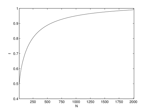
Figure 1: The fraction $f$ of times that the $x$ and $y$ are recognized as redundant for the variable $z$ (see the text), versus the number of samples $N$. $f$ is evaluated over $10^{6}$ repetitions.

consists of groups of redundant variables. Concerning the problem of finite sample size, we consider $N$ samples from eqs. (7), with $a=0.5$ and $b=0.4$, and estimate casualities on these data. In figure (1) we depict, as a function of $N$, the fraction $f$ of times that the $x$ and $y$ are recognized as redundant for the variable $z$ (with $A=0.4$); a large amount of data is needed to assess significative causality and so to discover redundancy. The present approach can thus be used only in applications such that a large number of samples is available.

Another example consists of a system of nine oscillators evolving according to noisy Kuramoto’s equations kuramoto :

$$\dot{\theta_{i}}=\omega_{i}+K\sum_{j=1}^{9}\;sin\left(\theta_{j}-\theta_{i}\right)+\xi_{i}(t);$$ (10)

We consider three groups of oscillators, each made of three oscillators with the same natural frequency, respectively $\omega=1,2,4$; the noise strength is $0.01$. Using the approach for circular variables, described in noipla , we find that the partition $\{A_{\ell}\}$ of the nine oscillators, maximizing the sum of the causalities between every pair of subsets

$$\Gamma=\sum_{\ell}\sum_{\ell^{\prime}\neq\ell}\delta^{u}(A_{\ell}\to A_{\ell^{\prime}}),$$

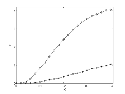
Figure 2: Concerning the system of nine oscillators described in the next, we depict the sum of the causalities between every pair of subsets $\Gamma$ (see the text) corresponding to the partitions $\{1,2,3\}\{4,5,6\}\{7,8,9\}$ (empty circles) and $\{1\}\{2\}\{3\}\{5\}\{6\}\{7\}\{8\}\{9\}$ (stars). Causalities are estimated over $5000$ samples for each value of $K$.

is $\{1,2,3\}\{4,5,6\}\{7,8,9\}$, corresponding to oscillators with the same natural frequency belonging to the same subset. In figure (2) we depict the optimal $\Gamma$ and the value of $\Gamma$ corresponding to the partition where each oscillator constitutes a set, versus the coupling $K$. It is clear that the maximization of $\Gamma$ reveals the structure of the system in this example.

Now we turn to consider a real application, i.e. EEG data from nineteen subjects suffering from migraine, under steady state flash stimuli (9 Hz) and repetitive transcranial magnetic stimulation (rTMS), a noninvasive method to excite neurons in the brain lanc . Migraine is a complex disorder of neurovascular origin whose pathophysiological basis is largely unknown. An altered cortical excitability may activate the trigemino-vascular system, but the question about a basal hypo or hyper cortical excitability is actually a matter of debate coppola . In a previous work prlss anomalous cortical synchronization in migraneurs under flash stimuli has been reported. A better understanding of migraine pathophysiology may improve its therapeutical approach: in this view, studies employing neurophysiological techniques, possibly supported by advanced methods of quantitative analysis, may give an aid to the knowledge of migraine pathophysiology valeriani . An important feature of migraine brain, is the tendency to hypersynchronization of alpha rhythms, which is influenced by anti-epileptic drugs detommaso . rTMS induces a cortical modulation that lasts beyond the time of stimulation fregni : its effects depend on the frequency of stimulations. In order to understand the physiological basis of abnormal neuronal oscillations in migraine brain, we apply 1 Hz rTMS over the occipital cortex, before performing repetitive flash stimulation. The records are 12 seconds long, sampled at 256 Hz: this EEG duration is representative of the pattern of brain responsiveness to light stimuli, as previously shown prlss . The signals are measured on seven channels (Fz,P3,P4,Cz,O1,Oz,O2) in three conditions basal (only flash stimuli) sham (placebo, i.e. flash stimuli and a fake magnetic stimulator) and rTMS (flash stimuli and magnetic stimulations) . As in the example above, for each target channel we exhaustively search for the partition of the remaining six channels which leads to the highest total causality $\Delta$ (averaged over the nineteen patients). In basal and sham conditions, we find that, for each target channel, the optimal partition is always a single set containing all the six remaining channels, in other words all the channels are redundant in these conditions. In presence of rTMS the causality pattern becomes more complex, and not all sets of variables are redundant w.r.t. the prediction of the others. All the six remaining channels are redundant for targets Fz,P4,O1,Oz; for the other channels the best partitions are

$$\begin{array}[]{rll}\{Fz,P4,O1,Oz,O2\}\{P3\}&\to&Cz\\ \{Fz,P4,O1,Oz,O2\}\{Cz\}&\to&P3\\ \{Fz,P4,O1,Oz\}\{CzP3\}&\to&O2.\end{array}$$ (14)

These relations suggest the presence of a new source of information, due to magnetic stimulations, corresponding to Cz and P3 channels. We also search for the partition of the seven channel maximizing the total causality between groups ($\Gamma$), averaged over the patients. We find that the best partition is $\{Fz,P4,O1,O2\}\{CzP3Oz\}$ for basal and sham conditions. For the TMS condition, instead, the best partition is $\{Fz,P4,Oz\}\{CzP3\}\{O1\}\{O2\}$; this result is consistent with the previous analysis as the channels Cz and P3 are grouped, see figure (3).

The change of the informational pattern, induced by occipital cortex inhibition, may confirm that neuronal oscillations are related to the state cortical excitability. Presently, we have no explanation about the significance of the specific Cz-P3 group related to rTMS effect, but we can assert that oscillations in migraine brain vary as a function of cortical excitability. The reliability of this pattern in migraine needs to be matched with a control group, so as to better understand the peculiar reactivity of migraine brain and to find the optimal way to influence it. Some remarks are in order. Averaging over patients is mandatory to reduce the effects due to the variability among subjects. Our results are obtained using the linear kernel and $m=1$, but the same partitions are obtained using the quadratic kernel and $m=2$ (application of cross-validation, on these data, suggests a low value of the order m; therefore we restrict our analysis to $m=1,2$). We find, in this real application, that the optimal partition maximizing the total causality is unique in all cases. It may happen, in other instances, that several partitions have the same total causality: in those cases prior information should be used to select one of the degenerate partitions.

Summarizing, in this work we have quantitatively developed the notions of redundancy and synergy in the frame of causality. We have proposed to generalize the standard multivariate Granger method in presence of redundant variables, by using the causality index without normalization, and analyzing the system as follows: (i) for a given target, the remaining variables are grouped so as to maximize the total causality and (ii) the whole set of variables is partitioned to maximize the sum of the causalities between groups. Analyzing real data from a neurophysiological experiments, the proposed approach was able to detect the informational pattern induced by magnetic stimulations.

Figure 3: The partitions of electrodes maximizing $\Gamma$ (see the text). Left: the optimal partition for Basal and Sham conditions. Right: the optimal partition in presence of TMS.

References

- (1) N. Wiener, The theory of prediction. In E.F. Beckenbach, Ed.,Modern mathematics for Engineers. (McGraw-Hill, New York, 1956).
- (2) C.W.J. Granger, Econometrica 37, 424 (1969).
- (3) Y. Chen, G. Rangarajan, J. Feng and M. Ding, Phys. Lett. A 324, 26 (2004).
- (4) K.J. Blinowska, R. Kus, M. Kaminski, Phys. Rev. E 70, 50902(R) (2004).
- (5) D.A. Smirnov, B.P. Bezruchko, Phys Rev. E 79, 46204 (2009); D.A. Smirnov, I. Mohkov, Phys Rev. E 80, 16208 (2009).
- (6) M. Dhamala, G. Rangarajan, M. Ding, Phys. Rev. Lett. 100, 18701 (2008).
- (7) K. Ishiguro, N. Otsu, M. Lungarella, and Y. Kuniyoshi, Phys Rev. E 77, 036217 (2008).
- (8) D. Marinazzo, M. Pellicoro, S. Stramaglia, Phys. Rev. Lett. 100, 144103 (2008).
- (9) J. Geweke, J. Am. Stat. Assoc. 79, 907 (1984).
- (10) D. Marinazzo, M. Pellicoro and S. Stramaglia, Phys. Rev. E 77, 056215 (2008).
- (11) S. Boccaletti, V. Latora, Y. Moreno, M. Chavez and D.U. Hwang, Physics Reports 424, 175-308 (2006).
- (12) K. Hlavackova-Schindler, M. Palus, M. Vejmelka, J. Bhattacharya, Physics Reports 441, 1 (2007).
- (13) M. Palus, V. Albrecht, I Dvorak, Phys. Lett. A 175, 203 (1993).
- (14) E. Schneidman, W. Bialek, M.J. Berry, Journal of Neuroscience 23 11539 (2003).
- (15) L.M. Bettencourt, V. Gintautas, and M.I. Ham, Phys. Rev. Lett. 100, 238701 (2008).
- (16) After a linear transformation, we may assume all the time series to have zero mean and unit variance.
- (17) Y. Kuramoto, Chemical oscillations, Waves and Turbulence. (Springer, Berlin, 1984).
- (18) L. Angelini, M. Pellicoro, S. Stramaglia, Phys. Lett. A 373, 2467 (2009).
- (19) A.T. Barker, R. Jalinous, I.L. Freeston, The Lancet 325, 1106 (1984).
- (20) G. Coppola, F. Pierelli, J. Schoenen, Cephalalgia 27, 1427 (2007).
- (21) L. Angelini et al., Phys. Rev. Lett. 93, 038103 (2004).
- (22) M. Valeriani, Clin. Neurophysiol. 116, 2717 (2005).
- (23) M. De Tommaso et al., Clin. Neurophysiol. 118, 2297 (2007).
- (24) F. Fregni et al., Lancet Neurol. 6, 188 (2007).