Quantum state transfer in a $XX$ chain with impurities

Abstract

One spin excitation states are involved in the transmission of quantum states and entanglement through a quantum spin chain, the localization properties of these states are crucial to achieve the transfer of information from one extreme of the chain to the other. We investigate the bipartite entanglement and localization of the one excitation states in a quantum $XX$ chain with one impurity. The bipartite entanglement is obtained using the Concurrence and the localization is analyzed using the inverse participation ratio. Changing the strength of the exchange coupling of the impurity allows us to control the number of localized or extended states. The analysis of the inverse participation ratio allows us to identify scenarios where the transmission of quantum states or entanglement can be achieved with a high degree of fidelity. In particular we identify a regime where the transmission of quantum states between the extremes of the chain is executed in a short transmission time $\sim N/2$, where $N$ is the number of spins in the chain, and with a large fidelity.

1 Introduction

Since the first works dealing with the entanglement shared by pairs of spins on a quantum chain, the translational invariance of the chain (and its states) has been exploited to facilitate the analysis of the problem [1, 2, 3]. Anyway, there is a number of problems which do not possess the property of being translationally invariant: semi-infinite chains, chains with impurities [4] or, in a more abstract sense, random quantum states [5]. These problems have localized quantum states whose properties strongly differ from those of translationally invariant quantum states.

Localized quantum states can be used to storage quantum information [6] and play an important role in the propagation of entanglement through a quantum spin chain [7]. This kind of states also appears in some models of quantum computers in presence of static disorder [8].

Since the localization of a quantum state is a global property it seems natural to study its properties using a global entanglement measure as, for example, the one proposed by Meyer and Wallach [9]. Giraud et al. [10] derived exact expressions for the mean value of the Meyer-Wallach entanglement for localized random vectors and studied the dependence of this measure with the localization length of the states. Viola and Brown [11] studied the relationship between generalized entanglement and the delocalization of pure quantum states. Of course there are other possibilities to study the relationship between localization of quantum states and entanglement. The bipartite entanglement and localization of one-particle states in the Harper model has been addressed by Li et al. [12], the entanglement entropy at localization transitions is studied in [13] and the localized entanglement in one-dimensional Anderson model in [14].

In many proposals of quantum computers the qubit energies can be often individually controlled, this corresponds to controllable disorder of a spin system. Besides, in these models, the effective spin-spin interaction is usually strongly anisotropic, it varies from the Ising coupling in nuclear magnetic resonance and other systems [15] to the $XY$-type or the $XXZ$-type coupling in some Josephson-junction-based systems [16]. The localization properties of one and two excitation states in the $XXZ$ spin chain with a defect was studied with some detail by Santos and Dykman [17], but they did not study the entanglement of the one and two excitation states.

In this paper we are interested in the behaviour of the localization and the bipartite entanglement of the pure eigenstates of a quantum chain with one impurity located in one extreme. It is well know that the presence of one impurity results in the presence of a localized state. If the strength of the impurity is large enough the energy of the localized state lies outside the band of magnons, also known as one spin excitation states [17]. The one spin magnons in a homogeneous chain are extended states [17].

As we will show, if the localization of a given state is measured with the inverse participation ratio there are two kinds of localized states, a) exponentially localized states that lie outside the band of magnons, and b) localized states that lie inside the band, whose number depends on the length of the chain and the strength of the impurity. This second kind plays a fundamental role in the transmission of quantum states through the chain. In most quantum state transfer protocols the state to be transferred is localized at one end of the quantum chain and the transmission is successful when the time evolution of the system produces an equally localized state at the other end of the chain. So it seems natural to investigate the time evolution of a localization measure to gain some insight about the problem of quantum state transfer.

So, the analysis of the time evolution of the inverse participation ratio, when the initial state consists in a single excitation located in one impurity, allows the identification of scenarios where the transmission of quantum states can be achieved for (comparatively) short times and with a very good fidelity. In this sense we extend some results obtained by Wójcik et al. [18].

The paper is organized as follows, in Section II we present the $XX$ model describing the quantum spin chain with a impurity. In Section III we analyze in some detail the spectrum of the one spin excitations and the eigenstates. In Section IV we present the results obtained for the inverse participation ratio for each one spin excitation eigenstate while the bipartite entanglement of the eigenstates is analyzed in Section V. Finally, in Section VI, we discuss the relationship between localization and transmission of quantum states.

2 Model

We consider a linear chain of $N$-qubits with $XX$ interaction. The coupling strengths are homogeneous except at one site, the impurity, where the coupling strength is different. The system is described by the Hamiltonian

$$H(\alpha)=\alpha J(\sigma_{1}^{x}\sigma_{2}^{x}+\sigma_{1}^{y}\sigma_{2}^{y})+\sum_{i>1}J(\sigma_{i}^{x}\sigma_{i+1}^{x}+\sigma_{i}^{y}\sigma_{i+1}^{y}),$$ (1)

where $\sigma^{\gamma}$ are the Pauli matrices, $J<0$ is the exchange coupling coefficient and $\alpha J$ is the impurity exchange strength, $\alpha=1$ corresponds to the homogeneous case.

Since the Hamiltonian commutes with $S_{z}=\Sigma_{i}\sigma_{i}^{z}$, the Hamiltonian $H(\alpha)$ has a block structure where each of them is characterized by the number of excited spins in the chain. Because we are interested in the transmission of a state with one excited spin from one end of the chain to the other, we focus on the eigenvectors of the one excitation subspace where the complete dynamics take place. To describe the eigenstates, we choose a basis described by the computational states of this subspace $|n\rangle=(\uparrow\uparrow...\uparrow\downarrow_{n}\uparrow...\uparrow)$, where $n=1,\ldots,N$ given a basis set size equals to the number of spins of the chain.

In this basis, the Hamiltonian $H$ is represented by a $N\times N$ matrix

$${\mathcal{H}}=\left(\begin{array}[]{ccccc}0&\alpha J&0&\dots&0\\ \alpha J&0&J&\dots&0\\ 0&J&0&\dots&0\\ \vdots&\vdots&\vdots&\ddots&J\\ 0&0&0&J&0\end{array}\right).$$ (2)

Implementations of this model could be realized, for example, with cold atoms confined in optical lattices [19, 20, 21, 22] or with nuclear spin systems in NMR [23, 24]. While in the first case an initial pure state in the one excitation subspace can be realized, in the spin ensemble situations of NMR an effective one excitation subspace is achieved by creating pseudo pure states where an excess of magnetization is localized on a given spin.

3 Energy spectrum and eigenstates

In this Section we briefly recall some known results about the spectrum and the eigenstates of the model emphasizing those features that are of interest in the following Sections.

The one excitation spectrum consists of $N$ eigenenergies denoted by $\left\{E_{1}\leq E_{2}\leq...\leq E_{N}\right\}$. Choosing the total number of spins even the spectrum results symmetrical with respect to zero ($E=0$ is not an eigenvalue), for any value of $\alpha$. Then $\left\{E_{1},...,E_{M}\right\}$ are negative values whereas $\{E_{M+1},...,E_{N}\}$ are positive, where $M=N/2$. In the homogeneous case ($\alpha=\alpha_{J}\equiv 1$), the energy spectrum lies between the values $\pm 2|J|$, this interval is usually call the band of eigenvalues. The size of the chain only changes the number of eigenvalues between those extreme values, becoming a continuous spectrum when $N\rightarrow\infty$.

Figure 1: The one excitation spectrum vs $\alpha$ for a spin chain with 40 spins. For $\alpha$ large enough the spectrum shows two isolated eigenenergies and one band $|E|\leq 2|J|$. The two isolated curves correspond to the minimal eigenenergy $E_{1}$ (continuous line) and the maximal eigenenergy $E_{N}$ (dashed line). At the critical value $\alpha_{c}$ the isolated energies go into the band causing a slight distortion on the behaviour of energies inside the band. In this figure we use $|J|=1$

The inhomogeneous case shows a different behaviour. For large enough $\alpha$ the minimal and the maximal eigenenergy become isolated from the band. There is a critical value $\alpha_{c}$ which separates the region of the spectrum where the energies make a band ($0<\alpha<\alpha_{c}$) from the region where the energies make a band with two isolated energies ($\alpha>\alpha_{c}$). The critical point $\alpha_{c}$ can be obtained analytically, and for large values of $N$, $\alpha_{c}\simeq\sqrt{2}$. We will further analyze this point later on.

For $\alpha\gg\alpha_{c}$ the minimal and maximal energies move apart from the band proportionally to $-\alpha$ and $+\alpha$ respectively. This behaviour is depicted in Figure 1.

Figure 1 shows that most of the eigenenergies seem to be fairly independent of $\alpha$, except for the minimal and maximal energies. But a more detailed study of the derivative of the eigenenergies with respect to $\alpha$ (see section V), shows two regions where the changes in the spectrum are more noticeable: (i) for $\alpha\sim 0$ two eigenenergies become degenerate because the system changes from a chain with $N$ coupled spins to a chain with $N-1$ coupled spins and an uncoupled spin; ii) for $\alpha\lesssim\alpha_{c}$ there is a number of avoided crossings between successive eigenenergies, because of the “collision” among the minimal (or maximal) eigenenergy and the band.

The eigenstates in the one excitation subspace $|\Psi_{E}(\alpha)\rangle$, whose eigenvalue equation is

$$H(\alpha)|\Psi_{E}(\alpha)\rangle=E|\Psi_{E}(\alpha)\rangle,$$ (3)

can be written as a superposition of the one excitation states

$$|\Psi_{E_{j}}(\alpha)\rangle=\sum_{n=1}^{N}\Psi_{n}^{(j)}\left|n\right\rangle,$$ (4)

where due to the symmetries of the spectrum

$${\Psi_{n}^{(j)}=(-1)^{n}\Psi_{n}^{(N-j+1)}.}$$ (5)

These coefficients $\Psi_{n}^{(j)}$ contain information about localization and entanglement properties of the eigenstates and, can be written as [17]

$$\Psi_{n}^{(j)}=de^{i\theta n}+d^{\prime}e^{-i\theta n}.$$ (6)

In a homogeneous chain, the eigenstates are wave-like superpositions of the one excitation states where the coefficients of the superpositions are given by (6) with $\theta$ real. In other case, $\alpha\neq 1$, the eigenstates within the band are very similar to the states of the homogeneous case (Figure 2 shows $\Psi_{n}^{(M)}$ for $\alpha=0.1$), but they differ in their coefficient on the impurity site. For $\alpha>\alpha_{c}$ the minimal eigenenergy state $|\Psi_{E_{1}}\rangle$ is quite different (similarly for $|\Psi_{E_{N}}\rangle$), its coefficients $\Psi_{n}^{(1)}$ decay exponentially (Figure 2 shows $\Psi_{n}^{(1)}$ for $\alpha=1.6$).

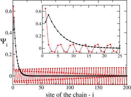
Figure 2: (color online) The coefficients $\Psi_{i}$ for two different eigenstates, $|\Psi_{E_{1}}(\alpha)\rangle$ with $\alpha=1.6$ (black squares) and $|\Psi_{E_{M}}(\alpha)\rangle$ with $\alpha=0.1$ (red circles). The lines are a guide to the eye. The states and the values of $\alpha$ were chosen to obtain equal values for their inverse participation ratios. The inset shows a zoom of the region near $i=1$.

It is rather simple to show the existence of a localized state when $\alpha\geq\sqrt{2}$. Using the ansatz $\Psi_{1}=u_{1}$ and $\Psi_{n}=(-1)^{n+1}e^{-n\kappa}$, for $n\geq 2$, to construct a state $\left|\Psi\right\rangle$, and replacing this state in Equation 3, after some algebra we obtain that

$$e^{2\kappa}=\alpha^{2}-1,$$ (7)

so, to obtain a localized state, the condition $e^{2\kappa}\geq 1$ implies that $\alpha\geq\sqrt{2}$. This has been discussed previously see, for example, the work of Stolze and Vogel [25]. In [25] the authors exploits the mapping between the $XX$ model with one excitation and a non-interacting fermion model with one particle.

The density matrix for each eigenstate is given by

$$\hat{\rho}_{E}(\alpha)=|\Psi_{E}(\alpha)\rangle\langle\Psi_{E}(\alpha)|,$$ (8)

which is a $N\times N$ matrix in the one excitation subspace.

4 Localization of the eigenstates

As stated above, the eigenenergies and eigenstates change according to the strength of the impurity considered in the system. To quantify and study their changes, we calculate the eigenstate localization as a function of the impurity strength. For that purpose we use the inverse participation ratio (IPR) [10],

$$L_{IPR}(\left|\Psi\right\rangle)=\frac{\sum_{n}^{{}^{N}}\Psi_{n}^{2}}{\sum_{n}^{N}\Psi_{n}^{4}},$$ (9)

where $\Psi_{i}$ are the coefficients of the superposition (4) of the state. When the state is highly localized (i.e. $\Psi_{i}$ is nonzero for only one particular value of $i$) $L_{IPR}(\left|\Psi\right\rangle)$ has its minimum value, 1, and when the state is uniformly distributed (ie. $\Psi_{i}=1/\sqrt{N}$ for all $i$) the IPR attains its maximum value, $N$. We call a state $|\Psi\rangle$ extended if $L_{IPR}(|\Psi\rangle)\sim{\mathcal{O}}(N)$, i.e. the IPR is of the same order of magnitude than the length of the chain.

From (5), two states whose eigenenergies are symmetric with respect to zero, say $|\Psi_{E_{j}}\rangle$ and $|\Psi_{E_{N-j+1}}\rangle$ where $j\leq N/2$, have the same IPR, i.e. $L_{IPR}(|\Psi_{E_{j}}\rangle)=L_{IPR}(|\Psi_{E_{N+1-j}}\rangle)$. As a consequence, each curve in Figure 3 is double and we consider the IPR only for the states $\left\{|\Psi_{E_{1}}\rangle,...,|\Psi_{E_{M}}\rangle\right\}$.

Figure 3: Localization measure ($L_{IPR}=\sum_{n}\Psi_{n}^{2}/\sum_{n}\Psi_{n}^{4}$) of different one-excitation eigenstates vs $\alpha$, for chain with $N=200$ spins. The values of $\alpha_{J}$ and $\alpha_{c}$ are shown. For $\alpha\gg\alpha_{c}$, the curves of the IPR for the all eigenstates, except those corresponding to the minimal and maximal eigenenergies, collapse into a single curve. For $\alpha>\alpha_{c}$ the curves with $L_{IPR}\sim 1$ correspond to the minimal and maximal eigenenergy states. The steep behaviour of these curves when $\alpha\rightarrow\alpha_{c}^{+}$ shows the change from well localized to extended states. The localized states, with low IPR, that appear for $\alpha<\alpha_{c}$ correspond to states with eigenenergies near the center of the band. Near $\alpha=0$ there are several localized states. Each curve is double as explained in the text.

Figure 3 shows the inverse participation ratio $L_{IPR}$ of several eigenstates $\{|\Psi_{E_{1}}\rangle,....,|\Psi_{E_{N}}\rangle\}$ as a function of the impurity coupling $\alpha$. We can identify three regions where the behaviour of the $L_{IPR}$ is qualitatively different. These regions are separated by $\alpha_{J}$ and $\alpha_{c}$, where at those values all eigenstates are equally localized.

The first region $0<\alpha<\alpha_{J}$ shows several localized eigenstates corresponding to energies close to zero, i.e. the center of the band. Calling $\alpha_{E_{j}}^{m}$ the value of $\alpha$ such that $L_{IPR}(E_{j},\alpha)=L_{IPR}(\left|\Psi_{E_{j}}(\alpha)\right\rangle)$ attains its minimum, the numerical results show that $L_{IPR}(\alpha_{E_{M}}^{m})<L_{IPR}(\alpha_{E_{M-1}}^{m})<...$ where $\alpha_{E_{M}}^{m}<\alpha_{E_{M-1}}^{m}<...$, i.e. the eigenstate is more localized as it is closer to $E=0$. Besides, the number of localized states increase with $N$.

In the second region $\alpha_{J}<\alpha<\alpha_{c},$ the eigenstates with energies close to the border of the band become more extended acquiring a IPR maximum near to $\alpha_{c}$. These peaks become sharper when $N$ grows. At $\alpha_{c}$, these eigenstates are again equally localized, but for values of $\alpha$ larger than $\alpha_{c}$, but very close to this value, the eigenstates become more localized. The size of the interval around $\alpha_{c}$ in which this critical behaviour can be observed depends on the size of the chain. This localization changes seem to be related to the avoided crossings in the spectrum previously described.

In the last region $\alpha>\alpha_{c}$ there are only two eigenstates highly localized that correspond to the minimal and maximal eigenenergies, $E_{1}$ and $E_{N}$. The other states are extended through $N-1$ sites of the chain.

We want to stress that the IPR gives a coarse description of the eigenstates, for example the states in Figure 2, despite of their very different behaviour, are equally localized if the measure of localization is the IPR, effectively $L_{IPR}(\Psi_{E_{1}})=L_{IPR}(\Psi_{E_{M}})\simeq 5.6$ for both states. This indicates that the IPR can not distinguish the exponentially localized state from the state with a wave-like superposition extended over the chain if the latter has its coefficient $\Psi_{1}$ large enough.

This shows that the IPR is a good tool to quantify changes in the system due to the introduction of a impurity spin, however it does not give information about where the eigenstate is localized. Moreover, it does not distinguish between quite different states as those described in Figure 2. Studying the coefficients of the eigenstates, we can observe where they are localized. In the present case they are mainly localized on the impurity site (see Figure 2). However, since we are interested in the transmission of initially localized quantum states, and that a successful transmission results in another localized state, the IPR could provide an easy way to identify when the transmission has taken place.

Since the IPR does not distinguish between the exponentially localized states that lie outside the band of magnons and the localized states inside the band it is necessary to study both kinds of states using a local quantity. In the next Section we study the entanglement between the impurity site and its first neighbor, this will allow us to classify the different eigenstates accordingly with its entanglement content.

5 Entanglement of the eigenstates

The bipartite entanglement between two qubits can be calculated using the Concurrence [28]. The Concurrence of two qubits in an arbitrary state characterized by the density matrix $\rho$ is given by

$$C(\rho)=max\{0,\lambda_{1}-\lambda_{2}-\lambda_{3}-\lambda_{4}\},$$ (10)

where the $\lambda_{i}$ are the square roots of the eigenvalues, in decreasing order, of the non-Hermitian matrix $\rho\widetilde{\rho}$. The spin-flipped state $\widetilde{\rho}$ is defined as

$$\widetilde{\rho}=(\sigma^{y}\otimes\sigma^{y})\rho^{*}(\sigma^{y}\otimes\sigma^{y}),$$ (11)

were $\rho^{*}$ is the complex conjugate of $\rho$ and it is taken in the computational basis $\{|\uparrow\uparrow\rangle,|\uparrow\downarrow\rangle\,|\downarrow\uparrow\rangle,|\downarrow\downarrow\rangle\}$. The concurrence takes values between 0 and 1, where 0 means that the state is disentangled whereas 1 means a maximally entangled state.

When considering a subsystem of two qubits on the chain, the concurrence is calculated with the reduced density matrix. The reduced density matrix for the spin pair $(i,j)$, $\rho_{E}^{(i,j)}(\alpha)$, corresponding to the eigenstate $|\Psi_{E}(\alpha)\rangle$ is given by

$$\rho_{E}^{(i,j)}(\alpha)={Tr}\left|\Psi_{E}(\alpha)\right\rangle\left\langle\Psi_{E}(\alpha)\right|={\mathrm{T}r}\hat{\rho}_{E}(\alpha),$$ (12)

where the trace is taken over the remaining $N-2$ spins leading to a $4\times 4$ matrix.

The structure of the reduced density matrix follows from the symmetry properties of the Hamiltonian. Thus, in our case the concurrence $C(\rho_{E_{k}}^{(i,j)})$ depends on $i$ and $j$, i.e. the indexes of the sites where the spin pair lies. Note that in the translationally invariant case $C(\rho_{E_{k}}^{(i,j)})$ depends only on $|i-j|$. In what follows $C_{i,j}=C_{i,j}(\rho_{E_{k}})=C(\rho_{E_{k}}^{(i,j)})$.

Using the definition $\langle\hat{A}\rangle=Tr(\hat{\rho}\hat{A})$, we can express all the matrix elements of the density matrix $\rho^{(i,j)}$ in terms of different spin-spin correlation functions. In particular, for nearest neighbors spins and the eigenstate $|\Psi_{E_{j}}\rangle$, we get

$$\rho_{E_{j}}^{(i,i+1)}=\left(\begin{array}[]{cccc}a_{j}&0&0&0\\ 0&b_{j}&\langle\sigma_{i}^{+}\sigma_{i+1}^{-}\rangle_{E_{j}}&0\\ 0&\langle\sigma_{i}^{+}\sigma_{i+1}^{-}\rangle_{E_{j}}^{*}&d_{j}&0\\ 0&0&0&0\end{array}\right),$$ (13)

where

$$a_{j}=\frac{1}{4}\langle(\sigma^{z}+I)_{i}(\sigma^{z}+I)_{i+1}\rangle_{E_{j}},$$ (14)

$$b_{j}=\frac{1}{4}\langle(\sigma^{z}+I)_{i}(I-\sigma^{z})_{i+1}\rangle_{E_{j}},$$ (15)

$$d_{j}=\frac{1}{4}\langle(I-\sigma^{z})_{i}(\sigma^{z}+I)_{i+1}\rangle_{E_{j}},$$ (16)

$I$ is the $2\times 2$ identity matrix, $\sigma_{i}^{\pm}=(\sigma_{i}^{x}\pm i\sigma_{i}^{y})/2$, and

$$\langle\ldots\rangle_{E_{j}}=\left\langle\Psi_{E_{j}}\right|\ldots\left|\Psi_{E_{j}}\right\rangle.$$ (17)

Thus, the concurrence results to be

$$C_{i,i+1}(\rho_{E_{j}})=\max\{0,2\mid\langle\sigma_{i}^{+}\sigma_{i+1}^{-}\rangle_{E_{j}}\mid,2\sqrt{|b_{j}d_{j}|}\}.$$ (18)

For the set of eigenstates that we are considering, the expression for the concurrence can be further simplified. After some algebra we get

$$b_{j}=(\Psi_{i+1}^{(j)})^{2},\quad d_{j}=(\Psi_{i}^{(j)})^{2},$$ (19)

and that

$$\langle\sigma_{i}^{+}\sigma_{i+1}^{-}\rangle_{E_{j}}=\Psi_{i+1}^{(j)}\Psi_{i}^{(j)}.$$ (20)

So, we get that

$$C_{i,i+1}(\rho_{E_{j}})=2\left|\Psi_{i+1}^{(j)}\Psi_{i}^{(j)}\right|.$$ (21)

Using the Hellmann-Feynman theorem, and the symmetry properties of the Hamiltonian, we find that

$$\frac{\partial E_{j}}{\partial\alpha}=2J\left\langle\Psi_{E_{j}}\right|\sigma_{1}^{+}\sigma_{2}^{-}\left|\Psi_{E_{j}}\right\rangle.$$ (22)

From the expression for the reduced density matrix $\rho^{(i,i+1)}$, (13), it is clear that when $\langle\sigma_{i}^{+}\sigma_{i+1}^{-}\rangle=0$ the reduced density matrix is diagonal and the bipartite entanglement is zero. Moreover, from (22), when $\frac{\partial E_{j}}{\partial\alpha}=0$ we have that $C_{12}(\rho_{E_{j}})=0$.

So, the concurrence for the first two spins in the eigenstate $|\Psi_{E_{j}}\rangle$ is given by

$$C_{12}=\left|\frac{1}{J}\frac{\partial E_{j}}{\partial\alpha}\right|.$$ (23)

We are interested in the relationship between localization and entanglement for the whole one spin excitation spectrum. In particular, we want to show that the bipartite entanglement of a given eigenstate, which is a local quantity, between the impurity site and its first neighbor detects the type of localization that the eigenstate possess.

First, we proceed to analyze the concurrence of the minimal eigenenergy state, $C_{1,2}(\rho_{E_{1}})$ as a function of $\alpha$, the behaviour of this quantity is shown in Figure 4. At first sight, it is clear that $C_{1,2}(\rho_{E_{1}})$ is different from zero where $L_{IPR}(\left|\Psi_{E_{1}}\right\rangle)$ (see Figure 3) is noticeable, and that $C_{1,2}(\rho_{E_{1}})\rightarrow 0$ when the eigenvalue enters into the band and, consequently, the eigenstate becomes extended.

So, when the minimal eigenenergy state is extended for $\alpha<\alpha_{c}$, the two first spins are disentangled and $C_{1,2}(\rho_{E_{1}})=0$ consistently with $\frac{\partial E_{1}}{\partial\alpha}=0$ from (23). At the critical point $\alpha_{c}$, the state starts to become localized increasing its degree of localization when $\alpha\gg\alpha_{c}$; in the same way, the pair of spins starts to became entangled and almost disentangled from the rest of the chain, i.e. $C_{1,2}(\rho_{E_{1}})\sim 1$.

Actually, the data shown in Figure 4 corresponds too to $C_{1,2}(\rho_{E_{N}}(\alpha))$, this can be seen by the following argument.

Figure 4: Entanglement between the first spin (the impurity site) and its nearest neighbor for the eigenstate of the minimal eigenenergy $E_{1}$. It is measured by the concurrence $C_{1,2}(\rho_{E_{1}})$ as a function of $\alpha$. When the state is localized, $\alpha>\alpha_{c}$, spins 1 and 2 are also entangled. Before the critical point($\alpha\leq\alpha_{c}$) when the state is extended, $C_{1,2}(\rho_{E_{1}})=0$ consistently with $\frac{\partial E_{1}}{\partial\alpha}=0$ for $\alpha\leq\alpha_{c}$ .

As in the case of the IPR, the concurrence $C_{12}$ for eigenstates with symmetrical eigenenergies respect to zero ($E_{j}$ and $E_{N-j+1}$) is the same. From Eqs. (5) and (23), it is straightforward to demonstrate the latter affirmation where

$$C_{12}(\rho_{E_{j}})=C_{12}(\rho_{E_{N-j+1}}),\quad j=1,\ldots,M,$$ (24)

since

$$\frac{\partial E_{j}}{\partial\alpha}=-\frac{\partial E_{N-j+1}}{\partial\alpha}.$$ (25)

Following with the analysis of the entanglement between the first two spin in the chain, we calculate the concurrence of the states with energies inside the bands. Figure 5 shows $C_{12}(\rho_{E_{j}})$ as a function of $\alpha$ for $j=2,\ldots,M$. Note that the same scenario is observed for $C_{12}(\rho_{E_{j}})$ with $j=N-1,\ldots,M+1$.

Figure 5: (color online) Concurrence $C_{12}(\rho_{E_{j}}(\alpha))$ as a function of the impurity strength $\alpha$, for $j=2,3,\ldots,100$. The results were obtained for a chain of $N=200$ spins. Each curve $C_{12}(\rho_{E_{j}}(\alpha))$ has a single peak. The peaks are ordered by eigenenergy, the rightmost peak corresponds to $C_{12}(\rho_{E_{2}}(\alpha))$ (red dashed line), the peak to its left corresponds to $C_{12}(\rho_{E_{3}}(\alpha))$, and so on. The leftmost peak corresponds to the curve with the highest eigenenergy shown in the figure, $E_{100}$ (blue dashed-dotted line), belong to the energy of the center of the band. The inset shows the concurrence $C_{12}(\rho_{E_{j}}(\alpha))$ for $j=2,\ldots 70$

From Figure 5, and calling $\alpha_{i}^{m}$ the abscissa where $C_{12}(\rho_{E_{i}}(\alpha))$ has its maximum, we observe that $\alpha_{M}^{m}<...<\alpha_{2}^{m}$ and $C_{12}(\rho_{E_{M}}(\alpha_{M}^{m}))>....>C_{12}(\rho_{E_{2}}(\alpha_{2}^{m}))$. This observation suggests that the ordering of the maxima of the concurrence $C_{12}$ for the different eigenstates follows closely the ordering dictated by the amount of localization of these eigenstates, i.e only the most localized states around the impurity site has a noticeable entanglement. We will use this observation as a guide to formulate a transmission protocol in the next Section.

As we have shown, the concurrence and the derivative of the energy are related in a simple way, see (23). On the other hand it is well known that the eigenvalues $E_{i}(\alpha)$ inside the band are rather insensitive to changes in $\alpha$, indeed $\partial E_{i}(\alpha)/\partial\alpha\simeq 0$ almost everywhere, except near an avoided crossing with other eigenvalue. In this sense, the behaviour shown by the concurrence in Figure 5 reflects the presence of successive avoided crossings between $E_{1}(\alpha)$ and $E_{2}(\alpha)$, between $E_{2}(\alpha)$ and $E_{3}(\alpha)$, and so on. The abscissa of the peak in the concurrence of a given eigenstate roughly corresponds to the point where the eigenvalue becomes almost degenerate.

As a matter of fact, the scenario depicted in Figure 5 is not only a manifestation of the avoided crossings in the spectrum, indeed it can be considered as a precursor of the resonance state that appears in the system when $N\rightarrow\infty$. Recently, Ferrón et al. [29] have shown how the behaviour of an entanglement measure can be used to detect a resonance state. In a chain a resonance state appears in the limit $N\rightarrow\infty$, however the peaks in the concurrence obtained for $N$ large, but finite, can be used to obtain approximately the energy of the resonance state [29, 30].

6 Transmission of states and entanglement

The effect of the localized states in the one magnon band is best appreciated looking at the dynamical behaviour of the inverse participation ratio. Figure 6 shows the behaviour of $L_{IPR}(|\psi(t)\rangle)$, where $|\psi(t)\rangle$ satisfies that

$$i\frac{d|\psi(t)\rangle}{dt}=H|\psi(t)\rangle,\quad|\psi(t=0)\rangle=|1\rangle,$$ (26)

for different values of $\alpha$. There are, at least, three well defined dynamical behaviours, each one associated to the number of localized states in the system, see Figure 3. Figure 6 a) ($\alpha=0.1$) shows the behaviour of $L_{IPR}$ when there is only one localized state at the center of the band; Figure 6 b) ($\alpha=0.4$) shows the dynamical behaviour of $L_{IPR}$ when there are several localized states; the panels c), d) and e) show the dynamical behaviour near the transition zone and, finally, f) shows the dynamical behaviour when the system have exponentially localized states.

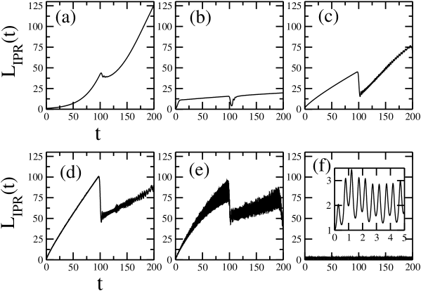
Figure 6: The panels show the dynamical behaviour of $L_{IPR}$ vs $t$, for different values of $\alpha$. a) $\alpha=0.1$, b) $\alpha=0.4$, c) $\alpha=1$, d) $\alpha=1.4$, e) $\alpha=1.5$ , and f) $\alpha=3$. In all the cases $|1\rangle$ is the initial condition. The inset in f) shows the small oscillations that characterize the behaviour of $L_{IPR}$ for $\alpha=3$, in this case the state of the system is localized even for very long times. In f) the initial excitation goes back and forth between the impurity site and the rest of the chain with a frequency given, basically, by the difference of energy between the two lowest eigenenergies. The steep change near $t\sim 100$, that can be observed in all the panels except in f), signals the “arrival” of the excitation to the end of the chain. Note that the refocusing, i.e. that the value of $L_{IPR}$ drops, is different in each regime, but in b) the refocusing leads to $L_{IPR}\sim O(1)$. The results were obtained for a chain with $N=200$.

We do not want to analyze completely the rich dynamical behaviour of $L_{IPR}$, however, from the point of view of the transmission of quantum states, it is clear that the regime shown in panel b) seems to be particularly useful. The panel b) shows that when the system has several localized eigenstates $|\psi(t)\rangle$ consists in a superposition of a reduced number of elements of the one excitation states, i.e the number of significant coefficients $\Psi_{i}$ is small compared with $N$. Besides, the refocusing of the state when the “signal” reaches the end of the chain (near $t\simeq 100$) leads to an smaller $L_{IPR}$ when $\alpha=0.4$ than for the other values of $\alpha$, compare panel b) with a), c), d) and e). The case shown in f) is rather different, in this case the superposition between the initial state $|1\rangle$ and the localized state is rather big, so $|\psi(t)\rangle$ remains localized even for very long times. This dynamical regime has been proposed to store quantum states [7] and, more generally, this kind of states with isolated eigenvalues has been proposed as a possible scenario to implement practically a stable qubit [31].

We want to remark some points: 1) for very small $\alpha$ there is a “refocusing” such that $L_{IPR}\sim 1$ for $t\sim{\mathcal{O}}(10^{4})$ when $N=200$. 2) The initial excitation that is localized in the impurities diffuses over the chain [32] so, for a given time $t$, the number of sites on the chain that are excited is given, approximately, by $L_{IPR}(t)$. The presence of localized states reduces this number and the speed of propagation. For $0.3\lesssim\alpha<\alpha_{c}$ the refocusing of the signal appears a $t\sim N/2$, this time is roughly independent of $\alpha$. For $\alpha\lesssim 0.3$ the time behaviour is more complicated but the refocusing times scales as $1/\alpha$, approximately, for fixed $N$, we will consider back this last point later.

We will use the regime b) identified in Figure 6 to implement the simplest transmission protocol, as suggested by Bose [26, 27], and the transmission of an entangled state. But, as our results suggest, we will place a second impurity at the end of the chain where the transmission should be detected. Locating an impurity at the end of the chain introduces a set of localized states around this site. The overall properties of the spectrum do not change, however the presence of localized states at the end of the chain would facilitate the transmission of states (or entanglement) from one end of the chain to the other.

Figure 7: The concurrence, $C_{A,N}$ (solid black line) and the fidelity $F_{1,N}$ (dashed black line) vs $t$ for a chain with $N=200$ spins.

In the simplest protocol of transmission (as described in [27]) the initial state, $|1\rangle$ evolves following the Hamiltonian dynamics, and the quality of the transmission is measured with the fidelity

$${F}=\langle 1|\rho_{out}(t)|1\rangle,$$ (27)

where $\rho_{out}(t)$ is the state at the end of the chain where the transmission is received, and $t$ is the “arrival” time.

For the transmission of an entangled state the protocol is slightly different, again we follow the protocol described in [27]. Using an auxiliary qubit $A$, and the first spin of the chain, the state

$$|\psi^{+}\rangle=\frac{1}{\sqrt{2}}(|\uparrow_{A}\downarrow_{1}\rangle+|\downarrow_{A}\uparrow_{1}\rangle)$$ (28)

is prepared. After the preparation of the initial state the systems evolves accordingly with its Hamiltonian and the concurrence between $A$ and the spin at the receiving end of the chain, $C_{A,N}(t)$, is evaluated.

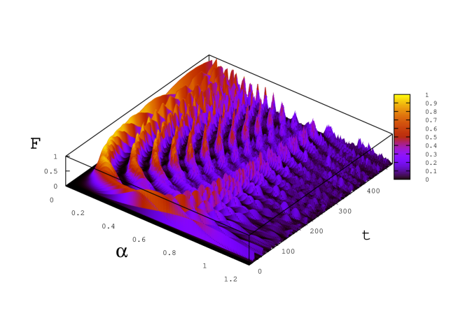
Figure 8: The fidelity of transmission versus the strength of the impurities and time. The fidelity presents a peak near $\alpha\simeq 0.6$ and $t\simeq 15$ for $N=31$. In this peak the fidelity is rather big.

Figure 7 shows the fidelity for the simplest transmission protocol and the concurrence between the auxiliary qubit and the last spin of the chain both as functions of the time. The strength of the interaction between the first and the second spin is the same that between the last and its neighbor, $\alpha J$, with $\alpha=0.4$, and the chain has $N=200$ spins. The maximum value of the fidelity and the concurrence are remarkably high. For our chain $C_{max}\simeq 0.9$, while for an unmodulated chain (with 200 spins) $C_{max}^{un}\simeq 0.23$ [26, 27]. It is worth to remark that this large value of the fidelity is not necessarily the larger possible tuning the value of $\alpha$.

As a matter of fact, that a chain with two symmetrical impurities outperforms a homogeneous one as a transmission device has been already reported in [18]. In that work, Wójcik et al. analyzed the transmission of quantum states modulating the coupling between the source and destination qubits. They shown that using small values of the coupling it is possible to obtain a fidelity of transmission arbitrarily close to one with the transfer time scaling linearly with the length $N$. Regrettably the resulting transfer time obtained in their work is quite large. Here we will extend their results showing that the transfer of quantum states is feasible for shorter transfer times with a very good fidelity ( $\gtrsim$ 0.9) while keeping the linear scaling between the transfer time and the length of the chain. To achieve this transfer scenario we will exploit the information provided by the IPR: for large enough values of $\alpha$ there is a time of order $N/2$ such that $L_{IPR}\sim 1$.

Figure 9: The data shown in the upper panel corresponds to the maximum fidelity of transmission achievable for times $t_{tr}\sim t_{IPR}\sim{\mathcal{O}}(N/2)$ for different chain lengths $N$ (squares), $\alpha_{opt}(N)$ (triangles) and the concurrence $C_{A,N}$(diamonds). The protocol of transmission is described in the text.

The identification of regimes where the transmission of quantum states can be achieved with large fidelity and for (relatively) short times is of great importance. The different dynamical regimes of the fidelity in a chain with two impurities is rather difficult to analyze except when $\alpha\rightarrow 0$, see [18]. Figure 8 shows the complex landscape of the fidelity of transmission versus the strength of the impurities and time. Some of the features shown by the fidelity in Figure 8 are best understood using the IPR. In particular, for $\alpha$ fixed, the first maximum of the fidelity as a function of the time coincides with a minimum of $L_{IPR}$. This observation, once systematized, provides the dynamical regime where the transmission can be achieved with large fidelity and always for times $\sim N/2$.

Our results about the time behaviour of the IPR show that for $t_{IPR}\sim{{\mathcal{O}}}(N/2)$ there is always a local minimum of the IPR (see Figure 6 b)). Since the state that is being transferred is well localized it is rather clear that we should look for times when the IPR attain local minima to identify where it is possible to achieve a good transmission. The time $t_{IPR}$ is rather independent of $\alpha$. So, optimizing the value of $\alpha$ in order to minimize the value of the minimum of the IPR at times $\sim t_{IPR}$ allow us to find the best fidelity achievable for time $t_{tr}\sim t_{IPR}$. We call $\alpha_{opt}(N)$ the value such that the the fidelity $F(t_{tr})$ attains its maximum for a given $N$ and for $t_{tr}\sim N/2$.

As Figure 7 shows, when the transfer of a given state takes place the fidelity presents a well defined maximum at time $t_{tr}\sim t_{IPR}\sim{\mathcal{O}}(N/2)$. The height of the maximum, $F_{max}$ is a smooth function of $\alpha$ for $\alpha>0.3$, and the same is valid for the transfer time $t_{tr}$.

Figure 9 summarizes our findings about the fidelity of transmission following the recipe outlined in the two paragraphs above. The upper panel shows the maximum transmission fidelity achievable for a chain of length $N$ and the corresponding optimum value of $\alpha$. As can be appreciated $F\gtrsim 0.8$ even for $N=400$. The maximum value of the fidelity is also well above the predicted for an unmodulated chain and above $2/3$ that is the highest fidelity for classical transmission of a quantum state. The lower panel shows the transmission time $t_{tr}$ vs $N$. The linear scaling of $t_{tr}$ with $N$ is rather clear.

It is clear that for an isolated chain the availability of a regime where $F\sim 1$, regardless of the time required to achieve the transfer, is interesting. However, in the presence of dynamical disorder or an “environment”, achieving a moderate fidelity for the transfer at shorter times seems a better option.

7 Discussion

There is enough evidence to affirm that the entanglement of quantum states whose eigenenergies present avoided crossings will show steep changes near of them ([29],[33], this work). In our case there is a number of avoided crossings that appears between successive levels, when $E_{1}$ comes into the band as $\alpha$ decreases from values larger than the critical. The avoided crossing between $E_{1}$ and $E_{2}$ is nearer to $\alpha_{c}$ than the avoided crossing between $E_{2}$ and $E_{3}$, and so on. This is the behaviour depicted in Figure (5). The width of the peak in $C_{12}$ of a given state (see Figure (5)) is related to the magnitude of the derivative of the eigenenergy of the state, the peak is sharper for $C_{12}(\rho_{E_{2}})$ and the successive peaks are more and more rounded.

As we have shown, locating impurities at both extremes of the chain allows to transfer more entanglement that an unmodulated chain if both impurities produce a number of localized eigenstates at each end of the chain. If a initially localized state is transmitted through the chain, at a posterior time the state is composed by the superposition of many propagating modes. The optimization of the couplings at the end of the chain allows the coherent superposition of many of those modes at some time $t_{tr}$, resulting in a large fidelity of transmission. The arrival time $t_{tr}$ is always $\geq N/2$. It could be interesting to compare the results presented in this work with the findings of Plastina and Apollaro ([34]) in the case of two diagonal impurities.

While IPR is an appealing quantity since it is very easy to calculate, we have shown that it is not possible to guess how much entanglement has a given state. The examples analyzed show that based on the IPR it is not possible to guess from it how much entanglement has a given state, anyway it remains an appealing quantity since it could be useful to identify dynamical regimes where the transmission of quantum states can be achieved. The example presented above, in which the tuning of the interaction between only a couple of spins improves the transmission, is encouraging. Of course the protocols for perfect transmission perform this task better, but at the cost of modulating all the interactions between the spins.

There is not, to our knowledge, a simple quantity that allows to relate, in a direct way, localization and entanglement. This subject will be object of further investigation.

References

References

- [1] Coffman V, Kundu J and Wootters W K 2000 Phys. Rev. A 61 052306
- [2] O’Connor K M and Wootters W K 2001 Phys. Rev. A 63 052302
- [3] Michalakis S and Nachtergaele B 2006 Phys. Rev. Lett. 97 140601
- [4] Osenda O, Huang Z and Kais S 2003 Phys. Rev. A 67 062321
- [5] Sommers H -J and Zyczkowski K 2004 J. Phys. A 37 8457; Giraud O 2007 ibid. 40 2793; Znidaric M 2007 ibid. 40 F105
- [6] Apollaro T J G and Plastina F 2007 Open Sys. and Information Dyn. 14 41
- [7] Apollaro T J G and Plastina F 2006 Phys. Rev. A 74 062316
- [8] Georgeot B and Shepelyansky D L 2000 Phys. Rev. E 62 3504; 2000 62, 6366
- [9] Meyer D A and Wallach N R 2002 J. Math. Phys. 43 4273
- [10] Giraud O, Martin J and Georgeot B 2007 Phys. Rev. A 76 042333
- [11] Viola L and Brown W G 2007 J. Phys. A: Math. Theor. 40 8109
- [12] Li H, Wang X and Hu B 2004 J. Phys. A: Math. Gen. 37 10665
- [13] Jia X, Subramaniam A R, Gruzberg I A and Chakravarty S 2008 Phys. Rev. B 77 014208
- [14] Li H and Wang X 2005 Mod. Phys. Lett. B 19 517
- [15] Chuang I L, Vandersypen L M K, Zhou X, Leung D B and Lloyd S 1998 Nature (London) 393 143
- [16] Makhlin Y, Schon G and Shnirman A 2001 Rev. Mod. Phys. 73 357
- [17] Santos L F and Dyckman M I 2003 Phys. Rev. B 68 214410
- [18] Wójcik A, Łuczak T, Kurzyński P, Grudka A, Gdala T and Bednarska M 2005 Phys. Rev. A 72 034303
- [19] Hartmann M J, Brandão F G S L and Plenio M B 2007 Phys. Rev. Lett. 99 160501.
- [20] Dorner U, Fedichev P, Jaksch D, Lewenstein M, and Zoller P 2003 Phys. Rev. Lett. 91 073601
- [21] Lewenstein M, Sanpera A, Ahufinger V, Damski B, Sen A, Sen U 2007 Adv. Phys. 56 243
- [22] Duan L-M, Demler E and Lukin M D 2003 Phys. Rev. Lett. 91 090402
- [23] Mádi Z L, Brutscher B, Schulte-Herbrüggen T, Brs̈chweileru R and Ernst R R 1997 Chem. Phys. Lett. 268 300
- [24] Álvarez G A, Mishkovsky M, Danieli E P, Levstein P R, Pastawski H M, and Frydman L 2010 Phys. Rev. A 81 060302(R)
- [25] Stolze J, Vogel M 2000 Phys. Rev. B 61 4026
- [26] Bose S 2007 Contemp. Phys. 48, 13
- [27] Bose S 2003 Phys. Rev. Lett. 91 207901
- [28] Wootters W K 1998 Phys. Rev. Lett. 80 2245
- [29] Ferrón A, Osenda O and Serra P 2009 Phys. Rev. A 79 032509
- [30] Pont F M, Osenda O, Toloza J H and Serra P 2010 Phys. Rev. A 81 042518
- [31] Michoel T, Mulhekar J and Nachtergaele B 2010 New J. Phys. 12 025003
- [32] Dente A, Bustos-Marún R A and Pastawski H M 2008 Phys. Rev. A 78 062116
- [33] González-Férez R and Dehesa J S 2003 Phys. Rev. Lett. 91 113001
- [34] Plastina F and Apollaro T J G 2007 Phys. Rev. Lett. 99 177210
- [35] Banchi L, Apollaro T J G, Cuccoli A, Vaia R and Verrucchi P 2010 Phys. Rev. A 82 052321