Jet gap jet events at Tevatron and LHC

Abstract:

We investigate diffractive events in hadron-hadron collisions, in which two jets are produced and separated by a large rapidity gap. Using a renormalisation-group improved NLL kernel implemented in the HERWIG Monte Carlo program, we show that the BFKL predictions are in good agreement with the Tevatron data, and present predictions which could be tested at the LHC.

In a hadron-hadron collision, a jet-gap-jet event features a large rapidity gap with a high$-E_{T}$ jet on each side ($E_{T}\!\gg\!\Lambda_{QCD}$). Across the gap, the object exchanged in the $t\!-\!channel$ is color singlet and carries a large momentum transfer, and when the rapidity gap is sufficiently large the natural candidate in perturbative QCD is the Balitsky-Fadin-Kuraev-Lipatov (BFKL) Pomeron [1]. Of course the total energy of the collision $\sqrt{s}$ should be big ($\sqrt{s}\gg E_{T}$) in order to get jets and a large rapidity gap.

Following the success of the forward jet and Mueller Navelet jet BFKL NLL studies [2], we use the implementation of the BFKL NLL kernel inside the HERWIG [3] Monte Carlo to compute the jet gap jet cross section, compare our results with the Tevatron measurement and make predictions at the LHC [4].

1 BFKL NLL formalism

The production cross section of two jets with a gap in rapidity between them reads

$$\frac{d\sigma^{pp\to XJJY}}{dx_{1}dx_{2}dE_{T}^{2}}={\cal S}f_{eff}(x_{1},E_{T}^{2})f_{eff}(x_{2},E_{T}^{2})\frac{d\sigma^{gg\rightarrow gg}}{dE_{T}^{2}},$$ (1)

where $\sqrt{s}$ is the total energy of the collision, $E_{T}$ the transverse momentum of the two jets, $x_{1}$ and $x_{2}$ their longitudinal fraction of momentum with respect to the incident hadrons, $S$ the survival probability, and $f$ the effective parton density functions [4]. The rapidity gap between the two jets is $\Delta\eta\!=\!\ln(x_{1}x_{2}s/p_{T}^{2}).$

The cross section is given by

$$\frac{d\sigma^{gg\rightarrow gg}}{dE_{T}^{2}}=\frac{1}{16\pi}\left|A(\Delta\eta,E_{T}^{2})\right|^{2}$$ (2)

in terms of the $gg\to gg$ scattering amplitude $A(\Delta\eta,p_{T}^{2}).$

In the following, we consider the high energy limit in which the rapidity gap $\Delta\eta$ is assumed to be very large. The BFKL framework allows to compute the $gg\to gg$ amplitude in this regime, and the result is known up to NLL accuracy

$$A(\Delta\eta,E_{T}^{2})=\frac{16N_{c}\pi\alpha_{s}^{2}}{C_{F}E_{T}^{2}}\sum_{p=-\infty}^{\infty}{\int\frac{d\gamma}{2i\pi}}\frac{[p^{2}-(\gamma-1/2)^{2}]\exp\left\{\bar{\alpha}(E_{T}^{2})\chi_{eff}[2p,\gamma,\bar{\alpha}(E_{T}^{2})]\Delta\eta\right\}}{[(\gamma-1/2)^{2}-(p-1/2)^{2}][(\gamma-1/2)^{2}-(p+1/2)^{2}]}$$ (3)

with the complex integral running along the imaginary axis from $1/2\!-\!i\infty$ to $1/2\!+\!i\infty,$ and with only even conformal spins contributing to the sum, and $\bar{\alpha}=\alpha_{S}N_{C}/\pi$ the running coupling.

Let us give some more details on formula 3. The NLL-BFKL effects are phenomenologically taken into account by the effective kernels $\chi_{eff}(p,\gamma,\bar{\alpha})$. The NLL kernels obey a consistency condition which allows to reformulate the problem in terms of $\chi_{eff}(\gamma,\bar{\alpha}).$ The effective kernel $\chi_{eff}(\gamma,\bar{\alpha})$ is obtained from the NLL kernel $\chi_{NLL}{\left({\gamma,\omega}\right)}$ by solving the implicit equation $\chi_{eff}=\chi_{NLL}{\left({\gamma,\bar{\alpha}\ \chi_{eff}}\right)}$ as a solution of the consistency condition.

In this study, we performed a parametrised distribution of $d\sigma^{gg\rightarrow gg}/dE_{T}^{2}$ so that it can be easily implemented in the Herwig Monte Carlo since performing the integral over $\gamma$ in particular would be too much time consuming in a Monte Carlo. The implementation of the BFKL cross section in a Monte Carlo is absolutely necessary to make a direct comparison with data. Namely, the measurements are sensititive to the jet size (for instance, experimentally the gap size is different from the rapidity interval between the jets which is not the case by definition in the analytic calculation).

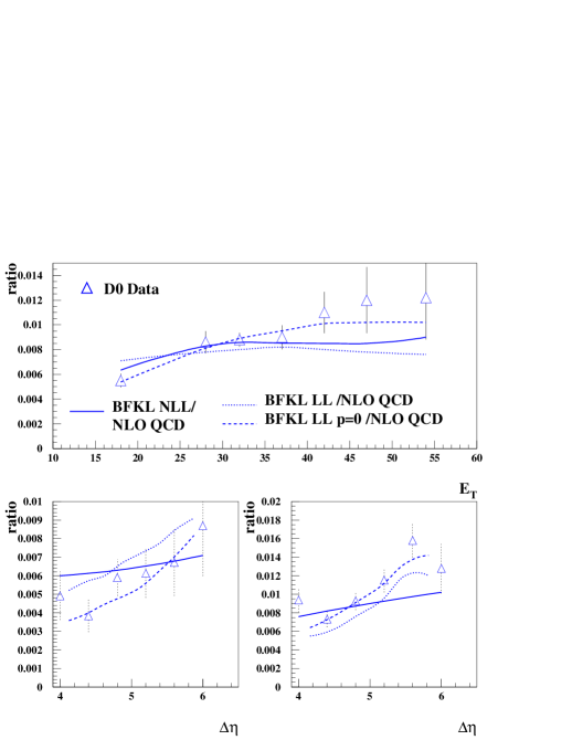
Figure 1: Comparisons between the D0 measurements of the jet-gap-jet event ratio with the NLL- and LL-BFKL calculations. For reference, the comparison with the LL BFKL with only the conformal spin component $p=0$ is also given.

2 Comparison with D0 and CDF measurements

Let us first notice that the sum over all conformal spins is absolutely necessary. Considering only $p=0$ in the sum of Equation 3 leads to a wrong normalisation and a wrong jet $E_{T}$ dependence, and the effect is more pronounced as $\Delta\eta$ diminishes.

The D0 collaboration measured the jet gap jet cross section ratio with respect to the total dijet cross section, requesting for a gap between -1 and 1 in rapidity, as a function of the second leading jet $E_{T}$, and $\Delta\eta$ between the two leading jets for two different low and high $E_{T}$ samples (15$<E_{T}<$20 GeV and $E_{T}>$30 GeV). To compare with theory, we compute the following quantity

$$Ratio=\frac{BFKL~{}NLL~{}HERWIG}{Dijet~{}Herwig}\times\frac{LO~{}QCD}{NLO~{}QCD}$$ (4)

in order to take into account the NLO order corrections on the dijet cross sections, where $BFKL~{}NLL$ $HERWIG$ and $Dijet~{}Herwig$ denote the BFKL NLL and the dijet cross section implemented in HERWIG. The NLO QCD cross section was computed using the NLOJet++ program [5].

The comparison with D0 data [6] is shown in Fig. 1. We find a good agreement between the data and the BFKL calculation. It is worth noticing that the BFKL NLL calculation leads to a better result than the BFKL LL one (note that the best description of data is given by the BFKL LL formalism for $p=0$ but it does not make sense theoretically to neglect the higher spin components and this comparison is only made to compare with previous LL BFKL calculations).

The comparison with the CDF data [6] as a function of the average jet $E_{T}$ and the difference in rapidity between the two jets is shown in Fig. 2, and the conclusion remains the same: the BFKL NLL formalism leads to a better description than the BFKL LL one.

3 Predictions for the LHC

Using the same formalism, and assuming a survival probability of 0.03 at the LHC, it is possible to predict the jet gap jet cross section at the LHC. While both LL and NLL BFKL formalisms lead to a weak jet $E_{T}$ or $\Delta\eta$ dependence, the normalisation if found to be quite difference leading to higher cross section for the BFKL NLL formalism.

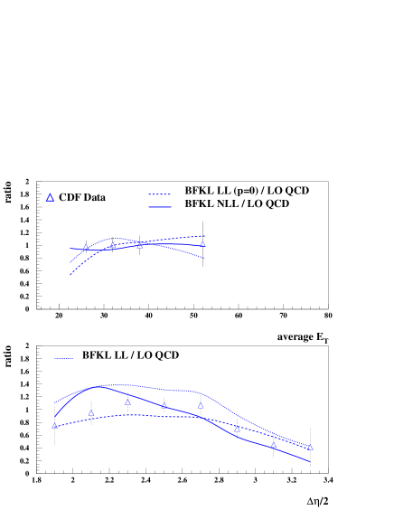
Figure 2: Comparisons between the CDF measurements of the jet-gap-jet event ratio with the NLL- and LL-BFKL calculations. For reference, the comparison with the LL BFKL with only the conformal spin component $p=0$ is also given.

References

- [1] V. S. Fadin and L. N. Lipatov, Phys. Lett. B 429, 127 (1998); M. Ciafaloni, Phys. Lett. B 429, 363 (1998);
- [2] O. Kepka, C. Royon, C. Marquet and R. B. Peschanski, Phys. Lett. B 655, 236 (2007); Eur. Phys. J. C 55, 259 (2008); C. Marquet and C. Royon, Phys. Rev. D 79, 034028 (2009).
- [3] G. Marchesini et al., Comp. Phys. Comm. 67, 465 (1992).
- [4] F. Chevallier, O. Kepka, C. Marquet, C. Royon, Phys. Rev. D79 (2009) 094019.
- [5] Z. Nagy and Z. Trocsanyi, Phys. Rev. Lett. 87, 082001 (2001).
- [6] B. Abbott et al., Phys. Lett. B 440, 189 (1998); F. Abe et al., Phys. Rev. Lett. 80, 1156 (1998).