Self-heating and its possible relationship to chromospheric heating in slowly rotating stars

Abstract

The efficiency of nonmodal self-heating by acoustic wave perturbations is examined. Considering different kinds of kinematically complex velocity patterns we show that nonmodal instabilities arising in these inhomogeneous flows may lead to significant amplification of acoustic waves. Subsequently, the presence of viscous dissipation damps these amplified waves and causes the energy transfer back to the background flow in the form of heat; viz. closes the “self-heating” cycle and contributes to the net heating of the flow patterns and the chromospheric network as a whole. The acoustic self-heating depends only on the presence of kinematically complex flows and dissipation. It is argued that together with other mechanisms of nonlinear nature the self-heating may be a probable additinal mechanism of nonmagnetic chromospheric heating in the Sun and other solar-type stars with slow rotation and extended convective regions.

1 Introduction

It is widely known that stars with outer convective zones, in terms of their chromospheric line emission, exhibit twofold behavior. Younger, rapidly rotating stars have the power of the chromospheric emission higher by 2-3 orders of magnitude than slowly rotating, older stars (Noyes et al., 1984). It is believed that the emission in these two classes of stars is related with different physical processes: the low emission of slow rotators represents the effect of acoustic, nonmagnetic heating, while the higher emission of fast rotators is caused by effects of magnetic activity (Schrijver et al., 1989). In the last decade it became increasingly clear that various slowly rotating, solar-type stars, with well-developed convection zones, have similar chromospheric emission. The available observational evidence suggests (Goodman, 2004) that this emission is caused, at least partially, by the upward propagation and dissipation of sound (acoustic) waves.

On the other hand, statistical analysis of existing ultraviolet (UV) emission data of solar-type stars across the H-R diagram, has shown the presence of a characteristic, well-pronounced “basal” level of chromospheric heating (Judge & Carpenter, 1998). It is commonly assumed that the heating may be caused by the nonlinear acoustic wave shock-heating mechanism, but the dynamics of this phenomenon is not completely understood. Moreover, the direct examination of Goddard High-Resolution Spectrograph data of several evolved stars, having similar “basal” levels of chromospheric activity, failed to detect a definite evidence in favor of the presence of acoustic waves, presumably a key component of the heating mechanism. Instead, in a number of cases, a counter-intuitive behavior, reminiscent of the solar transition region was detected, suggesting rather a magnetic heating mechanism for these stars. This controversy led to the tentative conclusion that upward-propagating shock waves do not necessarily dominate the observed radiative losses from chromospheres of stars exhibiting typical “basal” behaviour. More generally, the nonmagnetic nature of the basal components of convective, solar-type stars has been called in question.

In solar physics the problem of the chromospheric heating has been discussed ever since it was found out that the chromosphere is hotter than the photosphere. Originally it was proposed (Bierman, 1946; Schwarzschild, 1948) that the solar chromosphere is heated via the dissipation of acoustic waves generated by the overshooting convection zone turbulence. A theoretical model, determining the spectrum and power of these waves, had been developed on the basis of the Lighthill-Stein theory (Lighthill, 1952; Stein, 1967) of the convective zone acoustic wave emission. It was suggested that the dissipation of turbulently created acoustic waves may explain the observed chromospheric heating in the Sun. In this model it was supposed (Kalkofen, 2007) that the heating takes place in the granules. Alternatively, it may also occur in the lanes between granules (Lites et al., 1993), where the acoustic monopole emission may induce the chromospheric oscillations. At any rate both these scenarios were based on the assumption, confirmed by various observations of the solar chromosphere, that the acoustic mechanism of heating may be important in regions where the magnetic field is of a little significance both dynamically and energetically.

However, similarly to the situation with other solar-type stars, this explanation of the chromospheric heating has difficulties also for the Sun. The analysis of solar data from the SUMER(Solar Ultraviolet Measurements of Emitted Radiation) instrument on SOHO, analogously to the above-mentioned data from other slowly rotating, solar-type stars, revealed serious problems with the nonlinear acoustic-shock-wave interpretation and has underlined the necessity for the further investigation of this issue. Observations with TRACE (Transition Region And Coronal Explorer) NASA space telescope - revealed a very substantial (about $90\%$!) deficit in the energy flux required to heat the nonmagnetic, quiet solar chromosphere (Fossum & Carlsson, 2005a, b, 2006). Later some light on this puzzle was shed by numerical simulations with a three-dimensional hydrodynamic code. It was argued (Wedemeyer-Böhm et al., 2007; Cuntz et al., 2007) that this puzzling discrepancy may arise due to the limited spatial resolution of the TRACE, failing to detect most of the acoustic waves traveling in quiet-Sun inter-network regions of the chromosphere. In particular, Cuntz et al. (2007) discussed the problems of the limited sensitivity of TRACE while studying the three-dimensional solar chromospheric topology; they reconsidered the acoustic chromospheric wave energy flux and related this problem with the heating and emission of chromospheric basal flux for $\tau$ Ceti type stars. It was concluded that, contrary to claims by Fossum & Carlsson, high-frequency acoustic waves are sufficient to heat the nonmagnetic solar chromosphere.

Recently various alternative scenarios of the chromospheric heating for solar-type, cool stars with partially ionized chromospheres have been proposed. It was argued that the Farley-Buneman (Farley, 1963) plasma instability may provide the mechanism for conversion of the energy of convective motions of neutral atoms into the chromospheric heating (Fontenla, 2005; Fontenla et al., 2008). However Gogoberidze et al. (2008), taking into account the finite magnetization of the ions and Coulomb collisions, re-evaluated the instability for the solar chromosphere and argued that it could hardly be fully responsible for the observed level of quasi-steady heating.

Therefore, the problem of the chromospheric heating remains an actual and unsolved problem in the physics of slowly rotating, solar-type stars and the Sun. Putting the problem in plain words, it is observationally obvious that the chromospheres of stars with extended convective zones are hotter than their photospheres. This is true for both younger, rapidly rotating stars with magnetically active chromospheres and for older stars, with slower rotation rates and hydrodynamic, nonmagnetic chromospheres. Kalkofen (2007) has recently considered both possible mechanisms - the magnetic and the nonmagnetic (acoustic) ones - that might be responsible for the solar chromospheric heating. He argued (Kalkofen, 2008) that the emission of the nonmagnetic chromosphere exhibits some characteristic features of acoustic waves and no signatures of magnetic waves.

Still, in general, the problem is complicated. From the existing observational, theoretical and numerical studies of the “chromospheric heating problem” for cool, slowly rotating, solar-type stars, it turns out that the problem doesn’t have a single, broadly accepted solution. Rather, it seems likely that there may exist several different channels (mechanisms) of the chromospheric heating. It is a challenging task to specify these mechanisms and to provide at least a qualitative description of their relative importance. It seems evident that at any rate the chromospheric heating by acoustic waves takes place. The question is whether nonlinear heating by means of acoustic shock-waves is the only, or dominant, hydrodynamic channel of the heating or there are other acoustic processes of the energy transfer from waves to the medium that could lead to the chromospheric heating.

The role of the chromospheric flows and their kinematic complexity is possibly one of those important issues that has to be tested in the chromospheric heating context. It is well-known that the structure of the solar chromosphere is approximately spherically symmetric for about the first 2000 km. Higher layers show complex and variable fine structure, consisting of a wide variety of flow patterns - spicules, fibrils, surges (Bray & Loughhead, 1974; Athay, 1986; Zirin, 1988). Recent observations by Hinode strengthened this picture, showing that the chromosphere often hosts giant $H\alpha$ jets Kosugi et al. (2007); Nishizuka et al. (2008). It is now widely believed that the solar chromosphere, both in its active and quiet phases is highly dynamic and highly inhomogeneous consisting of numerous flows (“velocity patterns”) with different spatial/temporal time-scales and different geometries. These flows are closely related to the chromospheric network - a web-like structure seen in the emissions of the red line of hydrogen ($H\alpha$) and the ultraviolet line of calcium (Ca II K). The network is formed and maintained due to the presence of bundles of magnetic field lines ceaselessly shuffled and reshuffled by the fluid motions.

In particular, common ingredients of the solar chromosphere are spicules (small, jet-like ejections commonly observed throughout the chromospheric network), macro-spicules and solar tornadoes (Pike & Mason, 1998; Rogava et al., 2000). These flows are characterized by spatially inhomogeneous velocity fields: shear flows with a nontrivial geometry and a poorly known but considerable kinematic complexity. It is well-known that collective phenomena in shear flows are strongly affected by so-called nonmodal processes, related with the non-self-adjointness of the operator describing the linear dynamics of perturbations (Trefethen et al., 1993). These phenomena are especially robust and versatile in flows with nontrivial kinematics and geometries. In particular, it has been shown (Mahajan & Rogava, 1999) that under favourable conditions a hydrodynamic, linear system may exhibit strongly pronounced unstable regimes, where due to the efficient amplification of waves a large part of the mean flow kinetic energy is pumped into the unstable modes fostered by the flows. On the other hand, it was demonstrated that if viscous dissipation is present, the large amplitude, nonmodally amplified waves undergo viscous dissipation, leading to the conversion of the wave energy into thermal energy and corresponding “self-heating” (Rogava, 2004) of the “parent” flows.

The physics of the self-heating in a differentially moving medium (shear flow) is quite generic and comprises the following three steps: (a) The waves, originally, are excited spontaneously within the shear flow; (b) They undergo nonmodal amplification, they grow, extracting a part of the mean flow’s kinetic energy. These processes are quite efficient in neutral fluids (Butler & Farrell, 1992; Chagelishvili et al., 1997) and both in electrostatic (Rogava et al., 1997) and magnetized plasmas (Rogava et al., 2000). (c) Nonmodally amplified large-amplitude waves undergo, as the final stage of their evolution, viscous decay: they get damped and give their energy back to the “parent” flow in the form of heat.

Evidently the crucial element of this three-step process is the second one: nonmodal amplification of waves by the flow. The first and the last ones - spontaneous excitation of waves and their viscous damping - are routinely taking place in all kinds of continuous media. The possibility of the nonmodal amplification of collective modes in shear flows, however, creates a chance for the waves to amplify before they get damped! The energy needed for the amplification is drawn from the “reservoir” of the shear flow kinetic energy (Butler & Farrell, 1992). Eventual damping of these larger-amplitude waves and conversion of their excessive energy into the heat leads to the overall heating of the medium. Since this process converts, via the agency of nonmodally amplified waves, the kinetic energy of the flow into its thermal energy the process can be called self-heating.

Self-heating was originally described for acoustic waves in a hydrodynamic shear flow (Rogava, 2004), but later it was found (Li et al., 2006; Shergelashvili et al., 2006) that self-heating occurs in magnetohydrodynamic (MHD) shear flows too. The particularly robust nature of the nonmodal amplification in kinematically complex flows (Mahajan & Rogava, 1999; Rogava et al., 2003a) suggested that self-heating could be especially well pronounced in flows with complicated geometry and kinematics.

Since the solar chromosphere reveals the abundant presence of various nontrivial velocity patterns, and there is no reason to believe that chromospheric zones of other solar-type stars are any different it is reasonable to investigate the above mentioned mechanism in the context of the chromospheric heating for the slowly rotating, solar-type stars. In the present paper we consider the nonmodal self-heating mechanism in hydrodynamic, kinematically complex flows and study the energy dissipation rate of acoustic waves in the context of the possible relevance of this process to chromospheric flows.

The paper is arranged in the following way: In section II, we derive the equations governing the linear evolution of perturbations of the hydrodynamic system and consider the self-heating occurring within a kinematically complex flow. In section III, we apply this model to the chromospheric flows and solve the set of equations numerically for different parameter regimes. In section IV, we discuss the obtained results and outline the directions of further, more detailed, quantitative and applicative studies.

2 Main Consideration

In order to show the efficiency of the self-heating for acoustic waves generated, nonmodally amplified and viscously dissipated in kinematically complex shear flows, we consider the following standard hydrodynamic set, consisting of the equations of mass conservation:

$$D_{t}\rho+\rho\nabla\cdot{\bf V}=0,$$ (1)

the momentum conservation:

$$D_{t}{\bf V}=-\frac{1}{\rho}{\bf\nabla P}+\nu\Delta{\bf V},$$ (2)

and the polytropic equation of state:

$$P=C{\rho}^{1+1/n}.$$ (3)

In these equations, $D_{t}\equiv\partial_{t}+({\bf V}\cdot\nabla)$ denotes the convective derivative, $\rho$ is the density, ${\bf V}$ is the velocity, $\nu$ is the coefficient of kinematic viscosity and $n$ is the polytropic index.

The instantaneous values of the physical variables are expressed as sums of their equilibrium and perturbational components:

$$\rho\equiv\rho_{0}+\rho^{\prime},$$ (4)

$${\bf V}\equiv{\bf V_{0}}+{\bf V^{\prime}},$$ (5)

$$P\equiv P_{0}+P^{\prime}.$$ (6)

In the present study, for the sake of simplicity, the density of the fluid in the unperturbed state is assumed to be homogeneous ($\rho_{0}=\it{const}$).

Applying the standard procedure of linearization to Eqs. (1,2 and 3) in terms of Eqs. (4,5 and 6) one derives the following set of equations for the perturbed quantities:

$$\mathcal{D}_{t}\rho^{\prime}+\rho_{0}(\nabla\cdot{\bf V^{\prime}})=0,$$ (7)

$$\mathcal{D}_{t}{\bf V^{\prime}}+({\bf V^{\prime}}\cdot\nabla){\bf V_{0}}=-\frac{C_{s}}{\rho_{0}}{\bf\nabla\rho^{\prime}}+\nu\Delta{\bf V^{\prime}},$$ (8)

where $\mathcal{D}_{t}\equiv\partial_{t}+({\bf V_{0}}\cdot\nabla)$ and $C_{s}^{2}=dP_{0}/d\rho_{0}$.

Since there is no first-hand information about the velocity fields $\bf V_{0}$ of chromospheric flows and it is impossible to specify ‘typical’ or ‘standard’ flow patterns we do not limit this study with a narrowly chosen model for a prototype “parent” flow. Instead we will follow the approach originally developed and used in Mahajan & Rogava (1999) which applies to a broad range of possible flow patterns. Doing so we expand the velocity in a Taylor series in the vicinity of a point $A(x_{0},y_{0},z_{0})$. Preserving only linear terms we write:

$${\bf V}={\bf V}(A)+\sum_{i=1}^{3}\frac{\partial{\bf V}(A)}{\partial x_{i}}(x_{i}-x_{i0}),$$ (9)

where $i=1,2,3$ and $x_{i}=(x,y,z)$.

In Mahajan & Rogava (1999) it was shown that the initial set of linearized partial differential equations (7,8) is transformed to the set of ordinary differential equations by means of the usage of the following ansatz for the system’s physical variables:

$$F(x,y,z,t)\equiv\hat{F}(t)e^{\phi_{1}-\phi_{2}},$$ (10)

$$\phi_{1}\equiv\sum_{i=1}^{3}{K_{i}}(t)x_{i},$$ (11)

$$\phi_{2}\equiv\sum_{i=1}^{3}V_{i}(A)\int{K_{i}}(t)dt,$$ (12)

where $V_{i}(A)$’s are the unperturbed velocity components and $K_{i}(t)$’s are the wave vector components. The latter satisfy the following set of ordinary differential equations:

$${\bf\partial_{t}K}+{\bf S^{T}}\cdot{\bf K}=0,$$ (13)

where ${\bf S^{T}}$ is the transposed shear matrix with the shear matrix ${\bf S}$ (Mahajan & Rogava, 1999) defined as:

$${\bf S}=\left(\begin{array}[]{ccc}V_{x,x}&V_{x,y}&V_{x,z}\\ V_{y,x}&V_{y,y}&V_{y,z}\\ V_{z,x}&V_{z,y}&V_{z,z}\\ \end{array}\right),$$ (14)

with $V_{i,k}\equiv\partial V_{i}/\partial x_{k}$

Therefore, the ansatz reduces the mathematical aspect of the problem to the study of the initial value problem for the amplitudes $\hat{F}(t)$ of the spatial Fourier harmonics of the perturbations.

The background flow velocity comprises stretching and rotation of the flow field lines in the $XOY$ plane superimposed on a spatially inhomogeneous outflow along the $Z$ axis. In terms of the shear matrix it is written as (Rogava et al., 2003a, b):

$${\bf S}=\left(\begin{array}[]{ccc}\Sigma&A_{1}&0\\ A_{2}&-\Sigma&0\\ C_{1}&C_{2}&0\\ \end{array}\right).$$ (15)

Using the notation $f^{(1)}\equiv df/d\tau$ for temporal derivatives, where $\tau\equiv tK_{n}C_{s}$ is a dimensionless time variable, we can write down the equations for the perturbations, i.e. Eqs. (7,8), in the following, completely dimensionless form:

$$d^{(1)}+{\bf k}\cdot{\bf u}=0,$$ (16)

$${\bf u}^{(1)}+{\bf S}\cdot{\bf u}={\bf k}d-\overline{\nu}k^{2}{\bf u},$$ (17)

$$\textbf{k}^{(1)}+{\bf S^{T}}\cdot{\bf k}=0,$$ (18)

where the following dimensionless notations are used: $d\equiv-i\rho^{\prime}/\rho_{0}$, $\textbf{u}\equiv\textbf{V}^{\prime}/C_{s}$, $\sigma\equiv\Sigma/K_{n}C_{s}$, $a_{1,2}\equiv A_{1,2}/K_{n}C_{s}$, $R_{1,2}\equiv C_{1,2}/K_{n}C_{s}$, $\textbf{k}\equiv\textbf{K}/K_{n}$ and $\overline{\nu}\equiv\nu K_{n}/C_{s}$. Here $K_{n}$ is the value that will be used for the normalization of the wave vector. In particular, for the two-dimensional case we take $K_{n}\equiv K_{x}(0)$, while for the three-dimensional case - $K_{n}\equiv K_{z}$($=const$).

For the sake of the forthcoming analysis it is useful to define the total energy of the perturbations $E_{tot}$ and its components: the kinetic, $E_{kin}$, and the compressional, $E_{c}$, energies:

$$E_{tot}=E_{kin}+E_{c}=\frac{\textbf{u}^{2}}{2}+\frac{d^{2}}{2}.$$ (19)

It is straightforward to verify that:

$$E^{(1)}=-{\bf u}({\bf S}\cdot{\bf u})-\overline{\nu}k^{2}u^{2}.$$ (20)

For the evaluation of the efficiency of the self-heating we will also use the self-heating rate, defined as (Rogava, 2004):

$$\Psi(\tau)\equiv\frac{\overline{\nu}}{E(0)}\int_{0}^{\tau}k^{2}(\tau^{\prime})u^{2}(\tau^{\prime})d\tau^{\prime}.$$ (21)

3 Results

From previous studies it is known that self-heating is strong enough only if the instabilities are robust and swift enough to pump energy into the acoustic waves before they are dumped by the viscous dissipation. At the other hand, the viscosity must be strong enough to ensure the feedback mechanism, i.e. the transfer of the energy acquired by the waves back to the flow via viscous damping. It is reasonable to expect that strongly pronounced self-heating occurs only when there is a certain balance between the instability and viscous time-scales (Rogava, 2004; Li et al., 2006). Neither in the case of weak nonmodal amplification (i.e. when the waves do not have enough time to grow before the viscosity kicks in), nor in the case of negligibly weak viscosity (i.e. when the dissipation is not strong enough to dump the waves and heat the matter), the self-heating mechanism will not be efficient enough to ensure a substantial heating of the flow. From Eqs. (17), by means of a simple dimensional analysis, one can obtain a value of the maximum length-scale at which the viscous terms start becoming important: $\lambda_{cr}\leq\beta\nu/C_{s}$ (where $\beta$ is a dimensionless parameter). Below, we will see that an efficient self-heating can only happen for relatively small $\lambda\leq\lambda_{cr}$ length-scales.

In this section we intend to show how strong the self-heating could be for flows of different geometry and kinematics. Instead of restricting the consideration to a specific kind of chromospheric flow pattern we try to show the potential significance of this nonmodal process for various kinds of kinematically complex hydrodynamic flows.

As a first example, we consider the simplest, two-dimensional case. The Eqs. (16-18) then reduce to:

$$d^{(1)}+k_{x}u_{x}+k_{y}u_{y}=0,$$ (22)

$$u_{x}^{(1)}+\sigma u_{x}+a_{1}u_{y}=k_{x}d-\overline{\nu}k^{2}u_{x},$$ (23)

$$u_{y}^{(1)}+a_{2}u_{x}-\sigma u_{y}=k_{y}d-\overline{\nu}k^{2}u_{y},$$ (24)

$$k_{x}^{(1)}+\sigma k_{x}+a_{2}k_{y}=0,$$ (25)

$$k_{y}^{(1)}+a_{1}k_{x}-\sigma k_{y}=0.$$ (26)

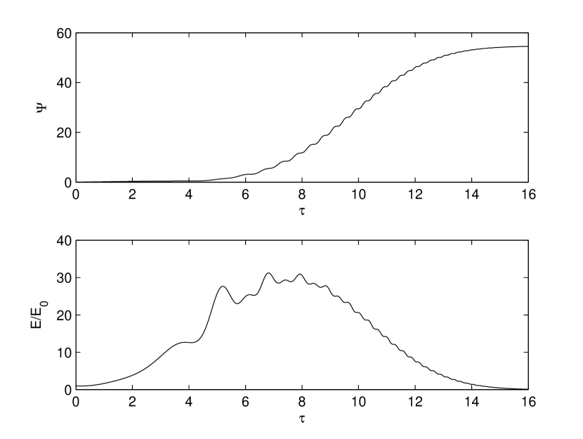
Figure 1: Temporal behaviour of the self-heating rate and the normalized total energy of perturbation. The set of parameters is: $a_{1}=-1.3$, $\sigma=a_{2}=0$, $k_{x0}=1$, $k_{y0}=-4$, $u_{x0}=0.2$, $u_{y0}=0$, $T=6000K$, $\lambda_{x}=160km$, $n=10^{11}cm^{-3}$.

Physical parameters of chromospheric flows in solar-type stars may have broad ranges of variability. In the low solar chromosphere, for instance, the flow velocity $V$, lies in the range $10-25\;$km/s , while the temperature, $T$, and the number density, $n$ are of the order of $5000-6000\;$K and $10^{11}\;$cm^-3, respectively (Sterling, 2000). The length-scale, $R$, of chromospheric structures may vary in the range $300-1500\;$km. One can easily show that for these values the nonzero components of the shear matrix $\sim V\lambda_{x}/(RC_{s})$ [see Eq. (29)] for $\lambda_{x}\sim R$ are of the order of unity. For the viscosity coefficient, we use the expression that is valid for a weakly ionized plasma, which appears to be a good approximation for the given range of temperatures (Goodman, 2000):

$$\nu=\frac{1}{3a_{0}^{2}n}\sqrt{\frac{k_{B}T}{m_{p}}},$$ (27)

where $a_{0}$ is the Bohr radius and $m_{p}$-the proton mass.

It is well-known that shear flows with a considerable kinematic complexity are subject to various, nonmodal instabilities, sometimes of a parametric nature (Mahajan & Rogava, 1999). The nonmodal evolution of perturbations strongly depends on the flow parameters and the wave characteristics. For instance, it was shown (Rogava et al., 2003a, b) that if $\Gamma\equiv\sigma^{2}+a_{1}a_{2}>0$, the system undergoes a linear instability, while for $\Gamma\leq 0$ the flow remains stable and exhibits an instability only for a narrow range of perturbation parameters.

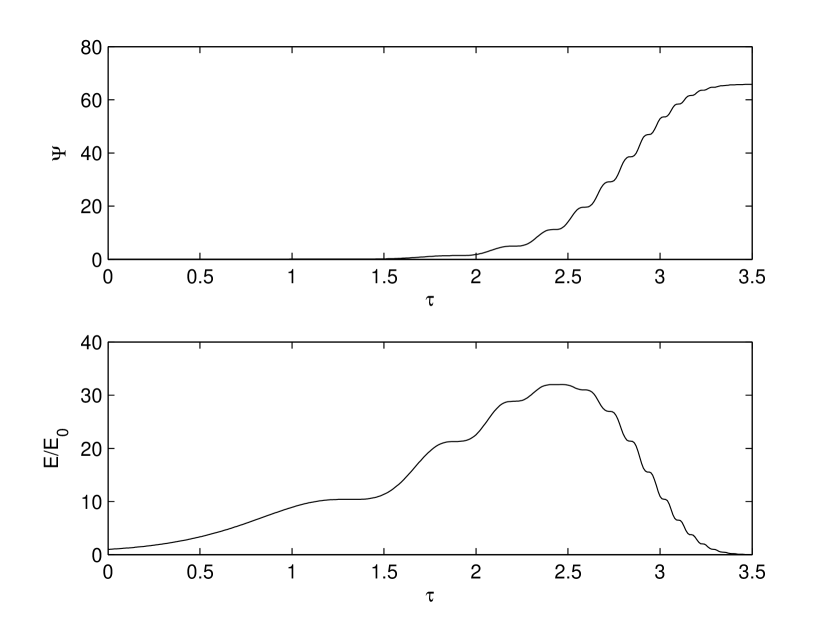
Figure 2: Temporal behaviour of the self-heating rate and the normalized total energy of perturbation. The set of parameters is: $a_{1}=a_{2}=-\sigma=1$, $k_{x0}=k_{y0}=1$, $u_{x0}=0.2$, $u_{y0}=0$, $T=6000K$, $\lambda_{x}=200km$, $n=10^{11}cm^{-3}$.

For the first example, we consider the case when the velocity shear is one-dimensional. In Fig. (1) the time evolution of the self-heating rate and the total energy of the acoustic perturbation for the case of a parametric instability ($\Gamma\leq 0$) are displayed. The set of parameters in this case was: $a_{1}=-1.3$, $\sigma=a_{2}=0$, $k_{x0}=1$, $k_{y0}=-4$, $u_{x0}=0.2$, $u_{y0}=0$, $T=6000\;$K, $\lambda_{x}=160\;$km, $n=10^{11}\;$cm^-3. From these plots it is clear that initially the unstable growth dominates over the viscous damping and the energy of the perturbation steadily increases. Gradually, however, the viscosity becomes more important and, as a result, the perturbation energy reaches its maximum level and starts decreasing until the perturbation completely disappears, giving back all the gained energy to the flow. Note that in this case the asymptotic value of the self-heating rate $\Psi_{\infty}\equiv\lim_{t\to\infty}\Psi(t)\simeq 60$ is reached.

The second example shows the case [see Fig. (2)] when the wave number vector components evolve exponentially ($\Gamma>0$). The set of parameters is: $a_{1}=a_{2}=-\sigma=1$, $k_{x0}=k_{y0}=1$, $u_{x0}=0.2$, $u_{y0}=0$, $T=6000\;$K, $\lambda_{x}=200\;$km, $n=10^{11}\;$cm^-3. The qualitative behaviour of the system is similar to the previous case: initially the perturbation rapidly grows at the expense of the background flow energy. But due to the exponential growth of the modulus of the wave vector the perturbation length-scale rapidly decreases, leading to the inevitable domination of the viscosity, which, in its turn, eventually damps the perturbation, converting its excessive energy into the thermal energy of the flow. The figure shows that the asymptotic self-heating rate in this case is about $\Psi_{\infty}\sim 70$.

Observational evidence suggests that the solar chromosphere is populated by three-dimensional fluxes, viz. flow patterns with nontrivial morphologies. An interesting class of these structures are the swirling macrospicules, also called the solar tornadoes Pike & Mason (1998), characterized by a helical motion of the plasma. It is plausible to expect that similar, highly nontrivial flow patterns may exist in chromospheric layers of other slowly rotating, solar-type stars. These are particularly intricate examples of flows with a very high degree of kinematic complexity! They may host various kinds of strongly-pronounced nonmodal shear instabilities Rogava et al. (2003a, b). Therefore, in our analysis, it is worthwhile to consider three-dimensional cases too and to check whether self-heating processes are equally or more efficient in them.

We consider the velocity configuration described by:

$${\bf V(r)}\equiv[0,r\Omega(r),U(r)],$$ (28)

with $\Omega(r)=\mathcal{A}/r^{\alpha}$ and $U=\;$const. In this case the shear matrix can be written in the following way (Rogava et al. (2003a)):

$${\bf S}=\left(\begin{array}[]{ccc}0&-\mathcal{A}/r^{\alpha}&0\\ \mathcal{A}\left(1-\alpha\right)/r^{\alpha}&0&0\\ R_{1}&R_{2}&0\\ \end{array}\right).$$ (29)

As an example, let us consider the case $\alpha=0.2$, $V_{\varphi}(R)=U$, and $r=R/2$. Fig. (3) shows the solution of Eqs. (16-18) for the following set of parameters: $R_{1}=R_{2}=-1$, $k_{z0}=-k_{x0}=1$, $k_{y0}=-5$, $u_{x0}=0.1$, $u_{y0}=u_{z0}=0$, $R=500km$, $U=20km/s$, $T=6000K$, $\lambda_{x}=200km$, $n=10^{11}cm^{-3}$. From the plots we see that the instability is so robust that the viscous dissipation fails to affect the perturbation evolution in a graphically visible way. Nevertheless, despite the seemingly insignificant contribution of viscous terms, their role in the self-heating process is as much instrumental as in all previously considered cases. The figure shows that the self-heating rate at the end of the given time interval ($\tau=20$) is quite high $\Psi\sim 500$.

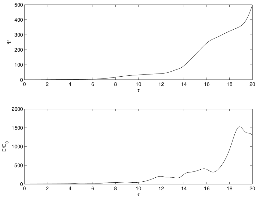
Figure 3: Temporal behaviour of the self-heating rate and the normalized total energy of perturbation. The set of parameters is: $\alpha=0.2$, $r=R/2$, $R_{1}=R_{2}=-1$, $k_{z0}=-k_{x0}=1$, $k_{y0}=-5$, $u_{x0}=0.1$, $u_{y0}=u_{z0}=0$, $R=500km$, $U=20km/s$, $T=6000K$, $\lambda_{x}=200km$, $n=10^{11}cm^{-3}$.

4 Discussion and Conclusions

Slowly rotating, older stars with well-developed convection zones (solar-type stars) feature similar chromospheric emission. Observations indicate that the emission is related to the dissipation of sound (acoustic) waves (Goodman, 2004) propagating from the photosphere to the chromosphere. The statistical analysis of the UV emission data from these stars shows the presence of a significant level of chromospheric heating (Judge & Carpenter, 1998). Commonly it is assumed that the heating is due to the dissipation of nonlinear acoustic waves. But the dynamics and the strength of the shock-heating mechanism are not well-understood and the nonmagnetic nature of chromospheric heating for solar-type stars has been recently doubted. From Goddard High-Resolution Spectrograph data of a number of solar-type stars no firm evidence was detected of the presence of acoustic waves. Quite on the contrary, in some cases the observational evidence seemed to be in favour of a magnetic mechanism for chromospheric heating for these stars. On the basis of this controversy it was surmised that upward-propagating shock waves do not necessarily govern radiative losses from the chromospheres of solar-type stars.

The situation is much the same in the context of solar physics. It is commonly believed that the solar chromosphere, in its quiet phase, in regions with negligibly weak magnetic field, has to be heated by acoustic waves. However, the energy flux of these waves, measured in the upper photosphere by TRACE, has been found to be insufficient to explain the radiative emission from the chromosphere. Wedemeyer-Böhm et al. (2007) and Cuntz et al. (2007), employing the three-dimensional hydrodynamical model (Wedemeyer-Böhm et al., 2004), have suggested that the spatial resolution of the TRACE is insufficient to resolve intensity fluctuations that occur on small spatial scales.

Kalkofen (2007) has also considered this assumption, implying that the spatial averaging by TRACE may serve as a qualitative explanation for the observed acoustic flux deficit. However, he found out that the standard hydrodynamical model was too oversimplified in the treatment of chromospheric energy exchange to provide a quantitative explanation of the suppression of the acoustic fluctuations. The mentioned hydrodynamic test (Wedemeyer-Böhm et al., 2007) was of a preliminary nature, because the hydrodynamic model on which the test was based involved temperature fluctuations exceeding those of the Sun. The shape of the acoustic spectrum observed with TRACE seemed to support the theory of wave generation in the solar convection zone even though the limited acoustic frequency range and the low energy flux of the observations did not allow to make any definitive conclusion (Kalkofen, 2007, 2008). That is why the conclusion was that “the heating mechanism of the chromosphere thus remained an open question” (Kalkofen, 2008).

The main goal of our present study was to show that the nonmodal self-heating by acoustic waves may serve as an additional source of chromospheric heating. We demonstrated the possibility of the efficient heating in chromospheric flows due to the presence of two basic factors: the existence of a spatially inhomogeneous, sufficiently complex velocity field (kinematically complex “flow patterns”), and the existence of viscous damping.

The self-heating is efficient when some necessary conditions upon the flow characteristics, for instance the kinetic energy budget of the mean flow, are met. The energy of the regular motion has to serve as an ample energy reservoir for the growing waves. Therefore, it is reasonable to consider the kinetic energy density of the flows in chromospheric structures and to compare it with the energy density of unstable modes.

Let us suppose that the characteristic velocity and the mass density of a chromospheric structure (e.g., a macro-spicule, a solar tornado, or a jet-like surge) are $V$ and $\rho$, respectively. The kinetic energy density can be expressed by:

$$E_{kin}\approx\frac{\rho V^{2}}{2}.$$ (30)

For the initial energy of the induced mode one gets [see Eq. (19)]:

$$E_{ind}=\frac{\rho C_{s}^{2}}{2}\left(u_{0}^{2}+d_{0}^{2}\right).$$ (31)

The energy converted into the form of heat, at the other hand, is of the order:

$$E_{heat}\approx\Psi\frac{\rho C_{s}^{2}}{2}\left(u_{0}^{2}+d_{0}^{2}\right),$$ (32)

implying that each generated mode extracts a certain portion of the mean flow kinetic energy:

$$\eta\equiv\Psi\frac{C_{s}^{2}}{V^{2}}\left(u_{0}^{2}+d_{0}^{2}\right).$$ (33)

For the parameters used for Fig. (1) and Fig. (2) one can easily show that $\eta$ equals $\sim 0.5$ and for Fig. (3), $\eta\sim 1$, leading to the conclusion that for the cases shown in Fig. (1) and Fig. (2) about $50\%$ of the chromospheric structures’ kinetic energy has been extracted and given back to the flow in the form of heat and almost $\sim 100\%$ for the case presented in Fig. (3). It means that this process is quite efficient for the heating of the “parent” flow. Apparently, if a large part of energy is extracted from the flow patterns they could easily be destroyed by the self-inflicted process of self-heating. This circumstance, in turn, could contribute to the statistically average short lifetimes ($\sim 1-10\;$min) of the macrospicules. For example, the case shown in Fig. (1) is characterized by the typical timescale of the self-heating, $t\sim\tau\lambda/C_{s}$ being of the order of $5min$. On the other hand, during one complete cycle of the self heating, almost $50\%$ of the flow kinetic energy will be extracted. For Fig. (2) the same energy fraction is extracted from the mean flow, but the heating timescale would be $\sim 2min$. Rather different situation is shown in Fig. (3), where the viscosity is not enough to saturate the instability and as is seen from the plot, the perturbed energy is increased asymptotically. Nevertheless, the presence of viscous damping is still significant, because as we see from Fig. (3), the self-heating rate for $\tau=20$ equals $\sim 500$. On the other hand, we have already mentioned that $\eta\sim 1$, thus the considered mode can extract the mean flow kinetic energy in approximately $7min$. As is seen from these figures, the more complex is the kinematics of the flow, the more efficient is the self-heating process.

The results of the present study, being of a qualitative nature, indicate that nonmodal shear flow instabilities, coupled with the presence of the viscous dissipation, may ensure the net chromospheric heating by the agency of the flow patterns of sufficiently complex kinematic structure. The presence of magnetic fields cannot alter this qualitative picture. On the contrary, it is known that in magnetized helical flows nonmodal shear instabilities tend to become much more powerful (Rogava et al., 2003a, b); and it has been shown that self-heating in the MHD may be quite efficient both generally (Li et al., 2006) and in the astrophysical context (Shergelashvili et al., 2006). It makes us believe that if self-heating is able to heat nonmagnetic part of the chromosphere of a solar-type star, it will certainly do the same job in a magnetized chromosphere too. We plan to study this issue in detail in the near future.

In the standard, Biermann-Schwarzschild, scenario of heating of the solar chromosphere (Bierman, 1946; Schwarzschild, 1948) the velocity amplitude of upward-propagating acoustic waves grows due to the exponential decrease of the mass density with height; leading, in turn, to shock formation and dissipation of the acoustic waves and heating of the medium. The important feature of this mechanism is the exponential dependence of the mass density on height, because for a medium with $\rho=const$ this classic scenario does not work. Alternatively, the nonmodal self-heating works when the density is homogeneous! On the other hand, it crucially depends on the presence of the kinematically complex shear flow. It is reasonable to expect that in realistic situations, viz. in chromospheric structures where both density stratification and flows are present, these two mechanisms will be complementary and will serve as additional sources of the heating.

One of the goals of our future research will be also the study of the propagation of acoustic gravity waves in gravitationally stratified chromospheric flows in the presence of viscous dissipation. Both linear and nonlinear regimes of acoustic-gravity wave propagation in two- (Kalkofen et al., 1994) and three-dimensional (Bodo et al., 2000) hydrodynamics and in the presence of the temperature inhomogeneity (Bodo et al., 2001) have been previously studied. It is interesting to study the dynamics of these waves in the presence of velocity shear and viscous damping and to check whether the nonmodal self-heating influences these processes too.

In order to study the role of the shear-induced nonmodal instability for the problem of the chromospheric heating in slowly rotating, solar-type stars we considered the model of a simple, quite general velocity pattern and wrote down hydrodynamic equations governing the evolution of acoustic perturbations within this flow. We have solved these equations for several, representative examples of flow patterns and found out that the instability and the viscous damping might lead to quite efficient self-heating of the “parent” flows. Analyzing the kinetic energy budget of a typical chromospheric macro-spicule, we found out that the self-heating might extract a significant part of kinetic energy from the velocity pattern in time-scales of the same order as the lifetimes of the corresponding structures observed in the solar chromosphere. Therefore, it is quite logical to believe that self-heating of chromospheric flow patterns contributes to the overall heating of the chromosphere by converting a considerable part of their kinetic energy into heat and ultimately destroying these flow patterns.

References

- Athay (1986) Athay R.G., 1986, in Physics of the Sun, Vol. II, ed. P. A. Sturrock (Dordrecht: Reidel), 51
- Bierman (1946) Biermann L., 1946, Naturwissenschaften, 33, 118
- Bodo et al. (2000) Bodo G., Kalkofen W., Massaglia S., Rossi P., 2000, A&A, 354, 296
- Bodo et al. (2001) Bodo G., Kalkofen W., Massaglia S., Rossi P., 2001, A&A, 370, 1088
- Bray & Loughhead (1974) Bray R.J., Loughhead, R.E., 1974, The Solar Chromosphere (London: Chapman and Hall)
- Butler & Farrell (1992) Butler K.M., Farrell B. F., 1992, Phys. Fluids A, 4, 1637
- Chagelishvili et al. (1997) Chagelishvili G.D., Khujadze G.R., Lominadze J.G., Rogava A.D., 1997, Phys. Fluids, 7, 1955
- Craik & Criminale (1986) Craik A.D.D., Criminale W.O., 1986, Proc.R.Soc.Lond. A, 406, 13
- Cuntz et al. (2007) Cuntz M., Rammacher W., Musielak Z.E., 2007, ApJ, 657, L57
- Farley (1963) Farley D.T. Jr., 1963, JGR, 68, 6083
- Fontenla (2005) Fontenla J.M., 2005, A&A, 442, 1099
- Fontenla et al. (2008) Fontenla J.M., Peterson W.K., Harder J., 2008, A&A, 480, 839
- Fossum & Carlsson (2005a) Fossum A., Carlsson M., 2005a, ApJ, 625, 556
- Fossum & Carlsson (2005b) Fossum A., Carlsson M., 2005b, Nature, 435, 919
- Fossum & Carlsson (2006) Fossum A., Carlsson M., 2006, ApJ, 646, 579
- Gogoberidze et al. (2008) Gogoberidze G., Voitenko Yu., Poedts S., Goossens M., 2009, arXiv:0902.4426
- Goodman (2000) Goodman M.L., 2000, ApJ, 533, 501
- Goodman (2004) Goodman M.L., 2004, A&A, 424, 691
- Kalkofen et al. (1994) Kalkofen W., Rossi P., Bodo G., Massaglia, S., 1994, A&A, 284, 976
- Kalkofen (2007) Kalkofen W., 2007, ApJ, 671, 2154
- Kalkofen (2008) Kalkofen W., 2008b, J. Astrophys. Astr., 2008, 29, 163
- Kosugi et al. (2007) Kosugi T. et al., 2007, Sol. Phys., 243, 3
- Judge & Carpenter (1998) Judge P.G., Carpenter K.G., 1998, ApJ, 494, 828
- Lagnado et al. (1984) Lagnado R.R., Phan-Thien N., Leal, L.G., 1984, Phys. Fluids, 27, 1094
- Li et al. (2006) Li J.W., Chen Y., Li Z.Y., 2006, Phys. Plasmas, 13, 042101
- Lighthill (1952) Lighthill M.J., 1952, Proc. R. Soc. London, A, 211, 564
- Lites et al. (1993) Lites B.W., Rutten R.J., Kalkofen W., 1993, ApJ, 414, 345
- Mahajan & Rogava (1999) Mahajan S.M., Rogava A.D., 1999, ApJ, 518, 814
- Nishizuka et al. (2008) Nishizuka N., 2008, ApJ, 683, L83
- Noyes et al. (1984) Noyes R.E., Hartmann L.W., Baliunas S.L., Duncan, D.K., Vaughan, A.H., 1984, ApJ, 279, 763
- Pike & Mason (1998) Pike C.D., Mason H.E., 1998, Sol. Phys., 182, 333
- Rogava et al. (1997) Rogava A.D., Mahajan S.M. Berezhiani V.I.,, 1997, Phys. Plasmas, 12, 4201
- Rogava et al. (2000) Rogava A. D., Poedts S., Mahajan S.M., 2000, A&A, 354, 749
- Rogava et al. (2003a) Rogava A.D., Mahajan S.M., Bodo G., Massaglia S., 2003, A&A, 399, 421
- Rogava et al. (2003b) Rogava A.D., Bodo G., Massaglia S., Osmanov, Z., 2003, A&A, 408, 401
- Rogava (2004) Rogava A. D., 2004, Ap. Space Sci., 293, 189
- Schrijver et al. (1989) Schrijver C.J., Dobson A.K., Radick R.R., 1989, ApJ, 341, 1035
- Schwarzschild (1948) Schwarzschild M., 1948, ApJ, 107, 1
- Shergelashvili et al. (2006) Shergelashvili B.M., Poedts S., Pataraya A.D., 2006, ApJ, 642, L73
- Stein (1967) Stein R.F., 1967, Sol. Phys., 2, 385
- Sterling (2000) Sterling A. C., 2000, Sol. Phys., 196, 79
- Trefethen et al. (1993) Trefethen L.N., Trefethen A.E., Reddy S.C. Driscoll T.A., 1993, Sience, 261, 578
- Wedemeyer-Böhm et al. (2004) Wedemeyer-Böhm S. et al., 2004, A&A, 414, 1121
- Wedemeyer-Böhm et al. (2007) Wedemeyer-Böhm S., Steiner O., Bruls J., Rammacher, W., 2007, in ASP Conf. Ser. 368, The Physics of Chromospheric Plasmas, ed. P. Heinzel, I. Dorotovic, & R.J. Rutten (San Francisco: ASP), 93
- Zirin (1988) Zirin H., 1988, Astrophysics of the Sun (Cambridge: Cambridge Univ. Press)