Efficient analysis and representation of geophysical processes using localized spherical basis functions

Abstract

While many geological and geophysical processes such as the melting of icecaps, the magnetic expression of bodies emplaced in the Earth’s crust, or the surface displacement remaining after large earthquakes are spatially localized, many of these naturally admit spectral representations, or they may need to be extracted from data collected globally, e.g. by satellites that circumnavigate the Earth. Wavelets are often used to study such nonstationary processes. On the sphere, however, many of the known constructions are somewhat limited. And in particular, the notion of ‘dilation’ is hard to reconcile with the concept of a geological region with fixed boundaries being responsible for generating the signals to be analyzed. Here, we build on our previous work on localized spherical analysis using an approach that is firmly rooted in spherical harmonics. We construct, by quadratic optimization, a set of bandlimited functions that have the majority of their energy concentrated in an arbitrary subdomain of the unit sphere. The ‘spherical Slepian basis’ that results provides a convenient way for the analysis and representation of geophysical signals, as we show by example. We highlight the connections to sparsity by showing that many geophysical processes are sparse in the Slepian basis.

1 The spherical Slepian basis

We denote the colatitude of a geographical point $\mathbf{\hat{r}}$ on the unit sphere surface $\Omega=\{\mathbf{\hat{r}}:\|\mathbf{\hat{r}}\|=1\}$ by $0\leq\theta\leq\pi$ and the longitude by $0\leq\phi<2\pi$. We use $R$ to denote a region of $\Omega$, of area $A$, within which we seek to concentrate a bandlimited function of position $\mathbf{\hat{r}}=(\theta,\phi)$. We use orthonormalized real surface spherical harmonics [1, 2], thus expressing a square-integrable real function $f(\mathbf{\hat{r}})$ on the surface of the unit sphere as

$$f(\mathbf{\hat{r}})=\sum\limits_{l=0}^{\infty}\sum\limits_{m=-l}^{l}{f}_{lm}Y_{lm}(\mathbf{\hat{r}}),\qquad{f}_{lm}=\int_{\Omega}f\hskip 1.00006ptY_{lm}\,d\Omega,\quad\mbox{and}\quad\int_{\Omega}Y_{lm}Y_{l^{\prime}m^{\prime}}\,d\Omega=\delta_{ll^{\prime}}\delta_{mm^{\prime}}.$$ (1)

The Slepian basis for the domain $R$ is the collection of bandlimited functions

$$g(\mathbf{\hat{r}})=\sum\limits_{l=0}^{L}\sum\limits_{m=-l}^{l}g_{lm}Y_{lm}(\mathbf{\hat{r}})\qquad\mbox{for which}\qquad\lambda=\left.\int_{R}g^{2}(\mathbf{\hat{r}})\,d\Omega\right/\int_{\Omega}g^{2}(\mathbf{\hat{r}})\,d\Omega=\mbox{maximum}.$$ (2)

Maximizing equation (2) leads to the spectral-domain Hermitian, positive-definite eigenvalue equation

$$\sum\limits_{l^{\prime}=0}^{L}\sum\limits_{m^{\prime}=-l^{\prime}}^{l^{\prime}}D_{lm,l^{\prime}m^{\prime}}g_{l^{\prime}m^{\prime}}=\lambda\hskip 1.00006ptg_{lm},\quad\mbox{with}\quad D_{lm,l^{\prime}m^{\prime}}=\int_{R}Y_{lm}Y_{l^{\prime}m^{\prime}}\,d\Omega,\qquad 0\leq l\leq L,$$ (3)

but we may equally well rewrite eq. (3) as a spatial-domain eigenvalue equation:

$$\int_{R}D(\mathbf{\hat{r}},\mathbf{\hat{r}}^{\prime})\,g(\mathbf{\hat{r}}^{\prime})\,d\Omega^{\prime}=\lambda\hskip 1.00006ptg(\mathbf{\hat{r}}),\quad\mbox{with}\quad D(\mathbf{\hat{r}},\mathbf{\hat{r}}^{\prime})=\sum_{l=0}^{L}\left(\frac{2l+1}{4\pi}\right)\!P_{l}(\mathbf{\hat{r}}\cdot\mathbf{\hat{r}}^{\prime}),\qquad\mathbf{\hat{r}}\in\Omega,$$ (4)

where $P_{l}$ is the Legendre function of integer degree $l$, which arises in this setting as a consequence of the spherical harmonic addition theorem[1, 2, 3]. Eq. (4) is a homogeneous Fredholm integral equation of the second kind, with a finite-rank, symmetric, Hermitian kernel, and the finite set of bandlimited spatial “Slepian” eigensolutions $g_{1}(\mathbf{\hat{r}}),g_{2}(\mathbf{\hat{r}}),\ldots,g_{(L+1)^{2}}(\mathbf{\hat{r}})$ is orthonormal over the whole sphere $\Omega$ and orthogonal over the region $R$:

$$\int_{\Omega}g_{\alpha}g_{\beta}\,d\Omega=\delta_{\alpha\beta},\quad\mbox{and}\quad\int_{R}g_{\alpha}g_{\beta}\,d\Omega=\lambda_{\alpha}\delta_{\alpha\beta}.$$ (5)

When the concentration region is a circularly symmetric cap of radius $\Theta$ centered on the North Pole the solutions to eq. (4) break down by order $m$ and are separable in $\theta$ and $\phi$, and the colatitudinal parts $g(\theta)$, which depend only on $|m|$, are identical to those of a Sturm-Liouville equation which can be solved in the spectral domain by diagonalization of a simple tridiagonal matrix with an almost linear spectrum[3, 4]. We define a space-bandwidth product or ‘spherical Shannon number’ by the sum of the eigenvalues,

$$N=\sum_{\alpha=1}^{(L+1)^{2}}\lambda_{\alpha}=\sum_{l=0}^{L}\sum_{m=-l}^{l}D_{lm,lm}=\int_{R}D(\mathbf{\hat{r}},\mathbf{\hat{r}})\,d\Omega=(L+1)^{2}\,\frac{A}{4\pi}.$$ (6)

The complete set of bandlimited spatial Slepian eigenfunctions $g_{1},g_{2},\ldots,g_{(L+1)^{2}}$, irrespective of the particular region of concentration that they were designed for, are a basis for bandlimited scalar processes anywhere on the surface of the unit sphere[3, 5]. This follows directly from the fact that the spectral localization kernel (3) is real, symmetric, and positive definite: its eigenvectors $g_{1\hskip 0.70004ptlm},g_{2\hskip 0.70004ptlm},\ldots,g_{(L+1)^{2}\hskip 0.70004ptlm}$ form an orthogonal set, thus the Slepian basis functions $g_{\alpha}(\mathbf{\hat{r}})$, $\alpha=1,\ldots,(L+1)^{2}$ given by eq. (2) simply transform the same-sized limited set of spherical harmonics $Y_{lm}(\mathbf{\hat{r}})$, $0\leq l\leq L$, $-l\leq m\leq l$ that are a basis for the same space of bandlimited spherical functions with no power above the bandwidth $L$. After sorting the eigenvalues in decreasing order, this transformation orders the resulting basis set such that the energy of the first $N$ functions, $g_{1}(\mathbf{\hat{r}}),\ldots,g_{N}(\mathbf{\hat{r}})$, with eigenvalues $\lambda\approx 1$, is concentrated in the region $R$, whereas the remaining eigenfunctions, $g_{N+1}(\mathbf{\hat{r}}),\ldots,g_{(L+1)^{2}}(\mathbf{\hat{r}})$, are concentrated in the complimentary region $\bar{R}=\Omega-R$. As in the one- and two-dimensional case[6, 7, 8], therefore, the reduced set of basis functions $g_{1},g_{2},\ldots,g_{N}$ can be regarded as a sparse, global, basis suitable to approximate bandlimited processes that are primarily localized to the region $R$. The dimensionality reduction is dependent on the fractional area of the region of interest, i.e. the full dimension of the space $(L+1)^{2}$ can be “sparsified” to an effective dimension of $N=(L+1)^{2}A/(4\pi)$ when the signal of interest lies in a particular geographic region.

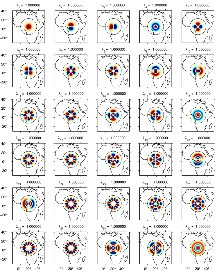
Figure 1: Bandlimited eigenfunctions $g(\theta,\phi)$ that are optimally concentrated within a circularly symmetric domain of colatitudinal radius $\Theta=18^{\circ}$ centered on $\theta_{0}=85^{\circ}$ and $\phi_{0}=18^{\circ}$. The bandwidth is $L=72$ and the rounded Shannon number $N=130$. The circle denotes the cap boundary. Blue is positive and red is negative and the color axis is symmetric, but the sign is arbitrary; regions in which the absolute value is less than one hundredth of the maximum value on the sphere are left white.

An example of Slepian functions on a circular region on the surface of the sphere can be found in Figure 1.

2 Problems in geophysics (and beyond)

With all of the foregoing established as fact and referring again to the literature cited so far for proof and further context, we return to considerations closer to home, namely the estimation of geophysical signals from noisy and incomplete observations collected at or above the surface of the spheres “Earth” or “planet”. We restrict ourselves to real-valued scalar measurements, contaminated by uncorrelated additive noise, which we may not know but which we shall describe by idealized models. We focus exclusively on data acquired and solutions expressed on the unit sphere. We have considered generalizations to problems involving satellite data collected at an altitude and/or potential fields elsewhere[9, 5, 4, 10]. Two different statistical problems arise in this context, namely, (i) how to find the “best” estimate of the signal given the data[5], and (ii) how to construct from the data the “best” estimate of the power spectral density of the signal in question[10]. In this contribution we limit ourselves to problem (i) as it is here that the connections to sparsity are most readily apparent.

Thus, let there be some data distributed on the unit sphere, consisting of ‘signal’, $n$ and ‘noise’, $s$, and let there be some region of interest $R\subset\Omega$, in other words, let

$$d(\mathbf{\hat{r}})=\left\{\begin{array}[]{ll}s(\mathbf{\hat{r}})+n(\mathbf{\hat{r}})&\mbox{if $\mathbf{\hat{r}}\in R$}\\ \mbox{unknown/undesired}&\mbox{if $\mathbf{\hat{r}}\in\Omega-R$}.\end{array}\right.$$ (9)

We assume that the signal of interest can be expressed by way of spherical harmonic expansion as in eq. (1), and that it is, itself, a realization of a zero-mean, Gaussian, isotropic, random process, namely

$$s(\mathbf{\hat{r}})=\sum\limits_{l=0}^{\infty}\sum\limits_{m=-l}^{l}s_{lm}Y_{lm}(\mathbf{\hat{r}}),\qquad s_{lm}=\int_{\Omega}s\,Y_{lm}\,d\Omega,\qquad\langle s_{lm}\rangle=0\quad\mbox{and}\quad\langle s_{lm}s_{l^{\prime}m^{\prime}}\rangle=S_{l}\,\delta_{ll^{\prime}}\delta_{mm^{\prime}}.$$ (10)

For convenience we furthermore assume that the noise is a zero-mean stochastic process with an isotropic power spectrum, i.e. $\langle n(\mathbf{\hat{r}})\rangle=0$ and $\langle n_{lm}n_{l^{\prime}m^{\prime}}\rangle=N_{l}\,\delta_{ll^{\prime}}\delta_{mm^{\prime}}$, and that it is statistically uncorrelated with the signal. We refer to power as white when $S_{l}=S$ or $N_{l}=N$, or, equivalently, $\langle n(\mathbf{\hat{r}})n(\mathbf{\hat{r}}^{\prime})\rangle=N\delta(\mathbf{\hat{r}},\mathbf{\hat{r}}^{\prime})$. Our objective is to determine the best estimate $\hat{s}_{lm}$ of the spherical harmonic expansion coefficients $s_{lm}$ of the signal. While in the real world there can be no limit on bandwidth, practical restrictions force any and all of our estimates to be bandlimited to some maximum spherical harmonic degree $L$, thus of necessity $\hat{s}_{lm}=0$ and $\hat{S}_{l}=0$ when $l>L$:

$$\hat{s}(\mathbf{\hat{r}})=\sum\limits_{l=0}^{L}\sum\limits_{m=-l}^{l}\hat{s}_{lm}Y_{lm}(\mathbf{\hat{r}}).$$ (11)

This limitation, combined with the statements eq. (9) on data coverage and the region of interest, naturally puts us back in the realm of ‘spatiospectral concentration’. As we shall see, solving the problem at hand will gain from involving ‘localized’ Slepian functions rather than, or in addition to, the ‘global’ spherical harmonics basis.

This leaves us to clarify what we understand by “best” in this context. While we adopt the traditional statistical metrics of bias, variance, and mean squared error to appraise the quality of our solutions[11, 12], the resulting connections to sparsity will be real and immediate, owing to the Slepian functions being naturally instrumental in constructing efficient, consistent and/or unbiased estimates of $\hat{s}_{lm}$ and/or $\hat{S}_{l}$. Thus, we define

$$v=\langle\hat{s}^{2}\rangle-\langle\hat{s}\rangle^{2},\qquad b=\langle\hat{s}\rangle-s,\qquad\epsilon=\hat{s}-s,\quad\mbox{and}\quad\langle\epsilon^{2}\rangle=v+b^{2},$$ (12)

where the lack of subscript indicates that we can study variance, bias and mean squared error of the estimate of the coefficients $\hat{s}_{lm}$ but also of their spatial expansion $\hat{s}(\mathbf{\hat{r}})$, or indeed of their power spectrum $\hat{S}_{l}$.

Signal estimation from noisy and incomplete spherical data

Spherical harmonic solution

Paraphrasing results elaborated elsewhere[5], we write the bandlimited solution to the damped inverse problem

$$\int_{R}(\hat{s}-d)^{2}\,d\Omega+\eta\int_{\bar{R}}\hat{s}^{2}\,d\Omega=\mbox{minimum},$$ (13)

where $\eta\geq 0$ is a damping parameter, by straightforward algebraic manipulation, as

$$\hat{s}_{lm}=\sum\limits_{l^{\prime}=0}^{L}\sum\limits_{m^{\prime}=-l^{\prime}}^{l^{\prime}}\left(D_{lm,l^{\prime}m^{\prime}}+\eta\bar{D}_{lm,l^{\prime}m^{\prime}}\right)^{-1}\int_{R}d\,Y_{l^{\prime}m^{\prime}}\,d\Omega,$$ (14)

where $\bar{D}_{lm,l^{\prime}m^{\prime}}$, the kernel that localizes to the region $\bar{R}=\Omega-R$, compliments $D_{lm,l^{\prime}m^{\prime}}$ given by eq. (3) which localizes to $R$. Given the eigenvalue spectrum of the latter, its inversion is inherently unstable, thus eq. (13) is an ill-conditioned inverse problem unless $\eta>0$, as has been well known, e.g. in geodesy[13, 14]. As can be easily shown, without damping the estimate is unbiased but effectively incomputable; the introduction of the damping term stabilizes the solution at the cost of added bias. And of course when $R=\Omega$, eq. (14) is simply the spherical harmonic transform, as in that case, eq. (3) reduces to eq. (1), in other words, then $D_{lm,l^{\prime}m^{\prime}}=\delta_{ll^{\prime}}\delta_{mm^{\prime}}$.

Slepian basis solution

We could seek a trial solution in the Slepian basis designed for this region of interest $R$ by writing

$$\hat{s}(\mathbf{\hat{r}})=\sum_{\alpha=1}^{(L+1)^{2}}\hat{s}_{\alpha}g_{\alpha}(\mathbf{\hat{r}}).$$ (15)

This would be completely equivalent to the expression in eq. (11) by virtue of the completeness of the Slepian basis for bandlimited functions everywhere on the sphere and the unitarity of the transform (2) from the spherical-harmonic to the Slepian basis. The solution to the undamped ($\eta=0$) version of eq. (13) would then be

$$\hat{s}_{\alpha}=\lambda_{\alpha}^{-1}\int_{R}d\hskip 1.00006ptg_{\alpha}\,d\Omega,$$ (16)

which, being completely equivalent to eq. (14) for $\eta=0$, would be computable, and biased, only when the expansion in eq. (15) were to be truncated to some finite $J<(L+1)^{2}$ to prevent the blowup of the eigenvalues $\lambda$. Assuming for simplicity of the argument that $J=N$, the essence of the approach is now that the solution

$$\hat{s}(\mathbf{\hat{r}})=\sum_{\alpha=1}^{N}\hat{s}_{\alpha}g_{\alpha}(\mathbf{\hat{r}})$$ (17)

will be sparse (in achieving a bandwidth $L$ using $N$ Slepian instead of $(L+1)^{2}$ spherical harmonic expansion coefficients) yet good (in approximating the signal as best as possible in the mean squared sense within the region of interest $R$) and of geophysical utility (assuming we are dealing with spatially localized processes that are to be extracted, e.g., from global satellite measurements)[15]. In light of the reasoning behind eqs (13)–(17), it is worth rereading the 1967 paper by W. M. Kaula[16], which, written long before the advent of Slepian functions and the associated mathematical machinery, paved the way for many other studies[17, 18, 5].

Bias and variance

In concluding this section let us illustrate another welcome by-product of our methodology, by writing the mean squared error for the spherical harmonic solution (14) compared to the equivalent expression (16) for the solution in the Slepian basis. We do this as a function of the spatial coordinate, in the Slepian basis for both, and, for maximum clarity of the exposition, using the contrived case when both signal and noise should be bandlimited as well as white (both stipulations being technically impossible to satisfy simultaneously). In the former case,

$$\langle\epsilon^{2}(\mathbf{\hat{r}})\rangle=N\sum_{\alpha=1}^{(L+1)^{2}}\lambda_{\alpha}[\lambda_{\alpha}+\eta(1-\lambda_{\alpha})]^{-2}g_{\alpha}^{2}(\mathbf{\hat{r}})+\eta^{2}S\sum_{\alpha=1}^{(L+1)^{2}}(1-\lambda_{\alpha})^{2}[\lambda_{\alpha}+\eta(1-\lambda_{\alpha})]^{-2}g_{\alpha}^{2}(\mathbf{\hat{r}}),$$

while in the latter, we obtain

$$\langle\epsilon^{2}(\mathbf{\hat{r}})\rangle=N\sum_{\alpha=1}^{N}\lambda_{\alpha}^{-1}g_{\alpha}^{2}(\mathbf{\hat{r}})+S\sum_{\alpha>N}^{(L+1)^{2}}g_{\alpha}^{2}(\mathbf{\hat{r}}).$$ (18)

All $(L+1)^{2}$ basis functions are required to express the mean squared estimation error, whether in eq. (2) or in eq. (18). The first term in both expressions is the variance, which depends on the measurement noise. Without damping or truncation the variance grows without bounds. Damping and truncation alleviate this at the expense of added bias, which depends on the characteristics of the signal, as given by the second term. In contrast to eq. (2), however, the Slepian expression (18) has disentangled the contributions due to noise/variance and signal/bias by projecting them onto the sparse set of well-localized and the remaining set of poorly localized Slepian functions, respectively. The estimation variance is felt via the basis functions $\alpha=1\rightarrow N$ that are well concentrated inside the measurement area, and the effect of the bias is relegated to those $\alpha=N+1\rightarrow(L+1)^{2}$ functions that are confined to the region of missing data.

When forming a solution to our problem in the Slepian basis by truncation according to eq. (17), changing the truncation level to values lower or higher than the Shannon number $N$ amounts to navigating the trade-off space between variance, bias (or “resolution”), and sparsity in a manner that is captured with great clarity by eq. (18). We refer the reader elsewhere[5] for more details.

3 Examples and applications

Sparsity of errors in approximation

Suppose that instead of eq. (13) we were to minimize

$$\int_{\Omega}(\hat{s}-d)^{2}\,d\Omega=\mbox{minimum},$$ (19)

which would lead to our forming the estimate from the partially observed data $d$ directly as

$$\hat{s}_{lm}=\int_{R}d\,Y_{lm}\,d\Omega.$$ (20)

While this might seem to be the natural approach in the absence of information outside the region of interest $R$, this would be equivalent to solving eq. (13) using a non-optimal damping constraint of $\eta=1$, as we have noted elsewhere[5], and eq. (14) furthermore shows this is so since $D_{lm,l^{\prime}m^{\prime}}+\bar{D}_{lm,l^{\prime}m^{\prime}}=\delta_{ll^{\prime}}\delta_{mm^{\prime}}$. Nevertheless, we use this example because it is simple and informative, and it has been studied by others before[14, 19]. If, for simplicity we assume that both signal and noise have a white power spectrum, the spectral error covariance matrix is

$$\langle\epsilon_{lm}\epsilon_{l^{\prime}m^{\prime}}\rangle=ND_{lm,l^{\prime}m^{\prime}}+S\bar{D}_{lm,l^{\prime}m^{\prime}},$$ (21)

as can be derived by combining eq. (20) with eqs (3) and (9)–(10). The errors are correlated, and are due to noise in the region $R$ where data exist, and contaminated by signal from the missing region $\bar{R}=\Omega-R$. It now makes immediate intuitive sense to desire a parameterization whose estimated coefficients have a diagonal covariance matrix. Let this parameterization be in terms of Slepian functions and thus this estimator

$$\hat{s}_{\alpha}=\int_{R}d\hskip 1.00006ptg_{\alpha}\,d\Omega,$$ (22)

which is to be contrasted with eq. (20), and the associated error covariance will be diagonal and given by

$$\langle\epsilon_{\alpha}\epsilon_{\beta}\rangle=[N\lambda_{\alpha}+S(1-\lambda_{\alpha})]\,\delta_{\alpha\beta}.$$ (23)

Eq. (23) follows from eq. (21) by the unitarity of the transform (2) and the properties (1) and (3).

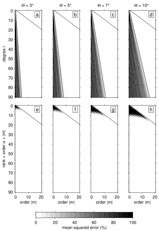
Figure 2: Error covariance of the solutions to the geodetic estimation problem for scalar data observed in a region $R$ in the presence of a ‘polar gap’, an axisymmetric pair of antipodal polar caps $\bar{R}=\Omega-R$ of radii $\Theta=0^{\circ},3^{\circ},5^{\circ},7^{\circ}$, and $10^{\circ}$, as shown. (a–d) Diagonal elements of the error covariance matrix, eq. (21), of the spherical harmonic solution (20). (e–h) Diagonal elements of the error covariance matrix, eq. (23), of the $L=90$ Slepian basis solution (22). The ordinate is the sum of the rank $\alpha$ of the Slepian function within a sequence of single absolute order and this order, $|m|$. The lines at $l=|m|$ in panels a–h mark the area of the space of spherical harmonics at degrees $l=0,\ldots,L$, and orders $|m|=0,\ldots,l$, while the lines at $|m|=(l+1/2)\sin\Theta_{0}$ in panels a–d delineate the approximate influence zone of the errors.

An example of this behavior can be found in Figure 2, where the mean squared errors $\langle\epsilon_{lm}^{2}\rangle$ and $\langle\epsilon_{\alpha}^{2}\rangle$ are plotted for the noiseless case, $N=0$, as a percentage of the signal strength, $S$. The geometry is that of a typical satellite survey characterized by a ‘polar gap’ $\bar{R}=\Omega-R$ consisting of a pair of axisymmetric caps at the North and South Pole, respectively, each one of various colatitudinal radii $\Theta=0^{\circ},3^{\circ},5^{\circ},7^{\circ}$, and $10^{\circ}$. The wedge shape of the errors in Figure 2a–d is bounded by the line $|m|=(l+1/2)\sin\Theta_{0}$. This relation substantiates earlier, heuristic, findings[19, 14]: it identifies $\Theta_{0}$ as the ‘turning colatitude’[2] separating the oscillatory from the evanescent parts of an asymptotic approximation of the Legendre functions at a given degree $l$ and order $m$. Compared to the error structure of the spherical harmonic solution (20) shown in Figure 2a–d, the error structure of the Slepian basis solution (22) shown in Figure 2e–h is decidedly more sparse.

Sparsity from geometry

Geophysical signals that are regional in nature are sparse in the Slepian domain — provided the Slepian basis constructed is commensurate with the localization of the signal itself. To illustrate this we focus no longer on estimating the field but rather on the representation and approximation of the solution once it has been obtained. To this end we will drop the hats, omit the angular brackets on all symbols, and ignore observational noise.

A bandlimited signal can be represented equally well in the spherical-harmonic as in any kind of Slepian basis of the same bandlimitation. When the signal is local and the chosen Slepian basis is similarly localized, approximating the function by the expansion truncated at the Shannon number will be advantageous

$$s(\mathbf{\hat{r}})=\sum\limits_{l=0}^{L}\sum\limits_{m=-l}^{l}s_{lm}Y_{lm}(\mathbf{\hat{r}})=\sum_{\alpha=1}^{(L+1)^{2}}s_{\alpha}g_{\alpha}(\mathbf{\hat{r}})\approx\sum_{\alpha=1}^{N}s_{\alpha}g_{\alpha}(\mathbf{\hat{r}}),$$ (24)

both because the quality of the approximation will be high in the region of interest and because the Shannon number of terms contributing to the reconstruction will be a significant savings over the full number of expansion coefficients. As per eq. (6) this sparsity is thus mostly “geometric” in origin and the efficiency gains are dependent on the area of the region of interest expressed as a fraction of the area of the entire unit sphere.

Using the double orthogonality definitions (5) it is easy to derive from eq. (24) that the mean squared error (mse) over the region of interest of such an approximation will depend on the signal terms neglected in the expansion, and that the “$R$-average mse” as a fraction of the $R$-average mean signal strength should be given by

$$\left.\int_{R}\epsilon^{2}(\mathbf{\hat{r}})\,d\Omega\right/\int_{R}s^{2}(\mathbf{\hat{r}})\,d\Omega=\left.\sum_{\alpha>N}^{(L+1)^{2}}s_{\alpha}^{2}\lambda_{\alpha}\right/\sum_{\alpha=1}^{(L+1)^{2}}s_{\alpha}^{2}\lambda_{\alpha}.$$ (25)

The quality of the regional approximation is high, because $\lambda_{\alpha}\approx 1$ when $\alpha\leq N$ and $\lambda_{\alpha}\approx 0$ when $\alpha>N$.

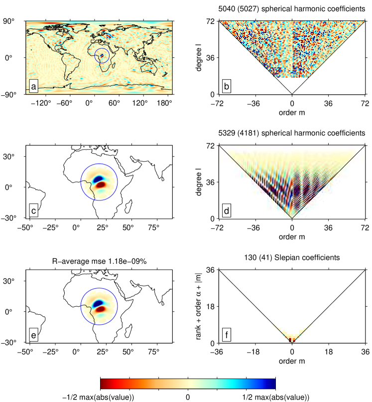
Figure 3: Global and local representations of the lithospheric magnetic field in the spherical-harmonic and Slepian bases. (a) Map of the radial component of the internal magnetic field at the Earth’s surface according to version 4.2s of the POMME model[20], bandpassed between spherical harmonic degrees 17 and 72, and (b) the spherical harmonic coefficients themselves. In total 5040 coefficients are needed to represent the global field, of which 5027 exceed a “1/1000” significance threshold of one thousandth of the maximum absolute value of all coefficients. Values below this relative threshold are left white in this and all other panels. (c) Map of what is known as the “Bangui anomaly”, a highly localized feature in central Africa. The anomaly was obtained by multiplying the global field, low-passed to degree 36, by the Slepian function of bandwidth 36 that is best concentrated to the circular area of radius $\Theta=18^{\circ}$, shown in blue. The resulting localized field is now bandlimited to degree 72, as can be seen in (d). Of the 5329 coefficients necessary to represent this anomaly, 4181 exceed the “1/1000” threshold. (e) An approximation of the same anomaly using the $N=130$ best-localized of the 5329 Slepian functions concentrated to the region and bandlimited to degree 72. Of the 130 coefficients only 41 exceed the “1/1000” threshold, as shown in (f), which has a truncated ordinate. The approximation in the region of interest is beyond reproach and the representation by the Slepian expansion, compared to the spherical harmonics, is truly sparse.

Figure 3 illustrates this by expanding the regional “Bangui anomaly” in the lithospheric magnetic field in both the spherical-harmonic and Slepian bases. As can be seen in Figure 3a–b, the radial component of the Earth’s main field, shown according to the POMME model[20] bandpass filtered to between degrees 17 and 72, contains some very prominent energy near Bangui, the capital of the Central African Republic. The origin of this anomaly remains debated[21]. Windowing a spatial expansion of the field between degrees 17 and 36 with a Slepian window of $L=36$ concentrated to a circular patch of radius $\Theta=18^{\circ}$ results in the rendition shown in Figure 3c–d. In the spherical harmonic domain, the windowed anomaly now contains energy between degrees $l=0-72$, as can be easily derived[9]. Almost 80% of the spherical harmonic expansion coefficients are significant in that their absolute value rises above a threshold of one thousandth of their maximum absolute value. Switching bases and expanding the signal in the $L=72$ Slepian basis localized to the same $\Theta=18^{\circ}$ region (i.e. those portrayed in Figure 1) results in a very small number of significant expansion coefficients. Indeed, the partial reconstruction using the first $N=130$ basis functions reveals that the anomaly is extremely well captured inside of the region of interest while the contribution to the signal is comprised of the energy of a mere 41 coefficients that are significant according to the same criterion, as shown in Figure 3e–f.

Sparsity from (geo)physics

It has long been known that earthquakes perturb the terrestrial gravity field[22]. Recently, thanks to the time-variable gravity measurements of the GRACE satellite pair[23], the study of such changes has received renewed attention[24, 15, 25, 26]. Following seismological convention[2], let us denote the hypocenter of an earthquake, which is to be considered as a point source, as $\mathbf{r}_{s}=(r_{s},\theta_{s},\phi_{s})$, and let us vectorize the symmetric ‘moment tensor’ as

$$\mbox{$\mathbf{M}$}=\left[\!\!\begin{array}[]{cccccc}M_{rr}&M_{\theta\theta}&M_{\phi\phi}&M_{r\theta}&M_{r\phi}&M_{\theta\phi}\end{array}\!\!\right].$$ (26)

In a coordinate system $\mathbf{r}^{\prime}=(r,\theta^{\prime},\phi^{\prime})$ that is centered on the epicenter of the earthquake, the first-order Eulerian gravitational potential perturbation in a spherically-symmetric non-rotating Earth is given by a sum over ‘spheroidal normal-mode’ eigenfunctions ${}_{n}P_{l}(r)$ (which depend on the Earth model, in our case prem[27]),

$$\phi^{\mathrm{E}1}(\mathbf{r}^{\prime})=\mbox{$\mathbf{M}$}\cdot\sum_{n=0}^{\infty}\sum_{l=0}^{\infty}{}_{n}\omega_{l}^{-2}{}_{n}P_{l}(r)\left(\frac{2l+1}{4\pi}\right){}_{n}\mbox{\boldmath$\mathcal{A}$}_{\hskip 0.52498ptl}(r_{s},\theta^{\prime},\phi^{\prime}),$$ (27)

where $l$ is the usual spherical harmonic degree, ${}_{n}\omega_{l}$ the temporal frequency, and the vector excitation amplitude

$${}_{n}\mbox{\boldmath$\mathcal{A}$}_{\hskip 0.52498ptl}(r_{s},\theta^{\prime},\phi^{\prime})=\sum_{m=0}^{\mathrm{min}(2,l)}\left[{}_{n}\mbox{$\mathbf{C}$}_{lm}(r_{s})\cos m\phi^{\prime}+{}_{n}\mbox{$\mathbf{S}$}_{lm}(r_{s})\sin m\phi^{\prime}\right]P_{lm}(\cos\theta^{\prime}),$$ (28)

with $m$ the usual spherical harmonic order, and with the associated Legendre function, $P_{lm}$, evaluated at the epicentral angular distance $\theta^{\prime}$. The vector functions ${}_{n}\mbox{$\mathbf{C}$}_{lm}$ and ${}_{n}\mbox{$\mathbf{S}$}_{lm}$ are combinations of normal-mode displacement eigenfunctions and their radial derivatives[2, 28], and need to be precomputed in the Earth model of choice.

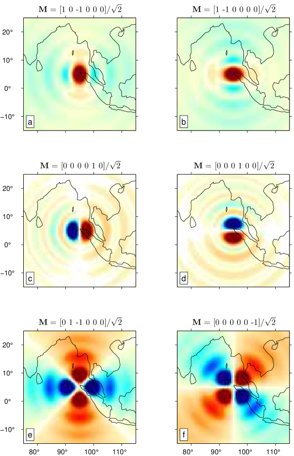
Figure 4: The patterns of gravitational potential perturbation owing to fictitious and idealized deviatoric double-couple point-source earthquakes occurring at 30 km depth underneath the island of Sumatra in the spherically symmetric Earth model prem[27], calculated from normal-mode theory[2] complete to degree $L=60$ . Blue is positive and red is negative; the color axes are symmetric. The components of the moment tensor, eq. (26), of these end-member cases are indicated by the title. (a)–(b) 45^∘-dip thrust faults. (c)–(d) Vertical dip-slip faults. (e)–(f) Vertical strike-slip faults. All focal mechanisms were normalized to unit scalar moment magnitude. The relative proportions of the magnitudes of the response shown in each row are 100%, 54%, and 34%, respectively.

Solutions (27) for a variety of end-member earthquake sources are shown in Figure 4. As suggested by the summation limits of eq. (28), the patterns with which earthquakes perturb the Earth’s gravity field have the symmetries of monopoles, dipoles, and quadrupoles[2, 28]. They should thus be eminently suitable to representation and amenable to analysis in the Slepian basis, in which, in other words, this type of geophysical signal is sparse.

To the standard treatment using spherical Slepian functions we add one sophistication, namely rotation about their center of figure. As we have noted the Slepian basis set on circularly symmetric domains is degenerate and separable into ‘colatitudinal’ eigenfunctions which are solutions to a Sturm-Liouville equation that can be solved spectrally with great ease[3, 5, 4], and order-dependent ‘longitudinal’ functions that control the axial symmetry. To compute the functions shown in Figure 1 we first determined the spherical harmonic expansion coefficients of the solutions to eq. (3) centered on the North Pole, and subsequently rotated those to the colatitude and longitude of the desired cap center. Now we shall rotate the resulting functions over a third Euler angle about their center.

We begin by a bait-and-switch for convenience — compared to Section 1 we will now work in the basis of complex surface spherical harmonics[1, 2], according to which the real Slepian and complex spherical harmonic expansion coefficients of the real signal $s(\mathbf{\hat{r}})$, $s_{\alpha}$ and $s_{lm}$, respectively, are related via the unitary transform

$$s_{\alpha}=\sum\limits_{lm}^{L}g^{*}_{\alpha\hskip 0.70004ptlm}s_{lm}\quad\mbox{and}\quad s_{lm}=\sum_{\alpha=1}^{(L+1)^{2}}g_{\alpha\hskip 0.70004ptlm}s_{\alpha},$$ (29)

where the $g_{\alpha\hskip 0.70004ptlm}$ form an $(L+1)^{2}\times(L+1)^{2}$ complex matrix. We shall here be concerned with obtaining the ‘localized’ coefficients $s_{\alpha}$ only when the spherical harmonic expansion coefficients $s_{lm}$ are “known”, e.g. by being given in the form of so-called ‘Level-2’ GRACE data products[29, 15]. Alternatives to this approach that can work directly from the raw data collected are discussed elsewhere[5, 30, 25].

Next, we adorn the Slepian basis functions, $g_{\alpha}$, their spherical harmonic expansion coefficients, $g_{\alpha\hskip 0.70004ptlm}$, and the Slepian expansion coefficients of the signal, $s_{\alpha}$, by three upper indices, $\omega$, $\theta$ and $\phi$, describing, respectively, the rotation about their center of symmetry, $0\leq\omega<2\pi$, and its colatitude, $0\leq\theta\leq\pi$, and longitude, $0\leq\phi<2\pi$. Thus, the “mother” Slepian basis set, concentrated over the circular region $R$ centered on the North Pole, bandlimited to $L$, and of Shannon number $N$, consists of the functions $g^{000}_{\alpha}(\mathbf{\hat{r}})$; they spawn a family of functions $g^{\phi\theta\omega}_{\alpha}(\mathbf{\hat{r}})$, $\alpha=1,\dots,(L+1)^{2}$, centered at the geographical locations $(\theta,\phi)$ on the unit sphere and rotated by $\omega$. For convenience we write no superscripts when $(\phi,\theta,\omega)=(0,0,0)$. The triad $(\phi,\theta,\omega)$ contains the three Euler angles that generate a Slepian basis of arbitrary orientation anywhere on the sphere: first, by rotation over $\omega$ around the $z$ axis, then by $\theta$ about the original $y$, and finally by $\phi$ around the original $z$ axis again. The spherical harmonic coefficients of the rotated $g^{\phi\theta\omega}_{\alpha}$ and the mother set $g_{\alpha}$ are then related by[1, 2]

$$g^{\phi\theta\omega}_{\alpha\hskip 0.70004ptlm}=\sum_{m^{\prime}=-l}^{l}\mathcal{D}^{(l)}_{mm^{\prime}}(\phi,\theta,\omega)\,g_{\alpha\hskip 0.70004ptlm^{\prime}},$$ (30)

where $\mathcal{D}^{(l)}_{mm^{\prime}}(\phi,\theta,\omega)$ is a $(2l+1)\times(2l+1)$ unitary transformation matrix of ‘generalized’ Legendre functions,[31, 32]

$$\mathcal{D}^{(l)}_{mm^{\prime}}(\phi,\theta,\omega)=e^{im\omega}d^{(l)}_{mm^{\prime}}(\theta)\,e^{im^{\prime}\phi},$$ (31)

duly noting that $d^{(l)}_{mm^{\prime}}(\theta)=d^{(l)}_{m^{\prime}m}(-\theta)$. It is now convenient[31, 33] to decompose a general rotation to $(\phi,\theta,\omega)$ into one over $(\phi-\pi/2,-\pi/2,\theta)$ followed by another over $(0,\pi/2,\omega+\pi/2)$. In that case eq. (30) can be rewritten as

$$g^{\phi\theta\omega}_{\alpha\hskip 0.70004ptlm}=\sum_{m^{\prime}=-l}^{l}\sum_{m^{\prime\prime}=-l}^{l}d^{(l)}_{mm^{\prime}}\!\left(\frac{\pi}{2}\right)d^{(l)}_{m^{\prime\prime}m^{\prime}}\!\left(\frac{\pi}{2}\right)e^{im(\omega+\pi/2)}e^{im^{\prime}\theta}e^{im^{\prime\prime}(\phi-\pi/2)}\,g_{\alpha\hskip 0.70004ptlm^{\prime\prime}}.$$ (32)

The expansion of the signal $s(\mathbf{\hat{r}})$ into the rotated Slepian basis $g^{\phi\theta\omega}_{\alpha}(\mathbf{\hat{r}})$ is given, as in eqs (15) and (29), by

$$s(\mathbf{\hat{r}})=\sum_{\alpha=1}^{(L+1)^{2}}s^{\phi\theta\omega}_{\alpha}\,g^{\phi\theta\omega}_{\alpha}(\mathbf{\hat{r}})\quad\mbox{and}\quad s^{\phi\theta\omega}_{\alpha}=\sum\limits_{lm}^{L}g^{\phi\theta\omega\hskip 0.70004pt*}_{\alpha\hskip 0.70004ptlm}s_{lm}.$$ (33)

Combining eqs (32)–(33) and rearranging the summations we can write the ‘fast Slepian expansion’ as a discrete Fourier transform[33, 34], to be calculated on a grid of frequencies by FFT of the operator $T_{m\hskip 0.875ptm^{\prime}m^{\prime\prime}}^{\alpha}$,

$$s^{\phi\theta\omega}_{\alpha}=\sum_{m=-L}^{L}\sum_{m^{\prime}=-L}^{L}\sum_{m^{\prime\prime}=-L}^{L}T_{m\hskip 0.875ptm^{\prime}m^{\prime\prime}}^{\alpha}\,e^{-im\omega}e^{-im^{\prime}\theta}e^{-im^{\prime\prime}\phi},$$ (34a)

$$T_{m\hskip 0.875ptm^{\prime}m^{\prime\prime}}^{\alpha}=\sum_{l=\max(|m|,|m^{\prime}|,|m^{\prime\prime}|)}^{L}d^{(l)}_{mm^{\prime}}\!\left(\frac{\pi}{2}\right)d^{(l)}_{m^{\prime\prime}m^{\prime}}\!\left(\frac{\pi}{2}\right)e^{i(m^{\prime\prime}-m)\pi/2}\,g^{*}_{\alpha\hskip 0.70004ptlm^{\prime\prime}}s_{lm}.$$ (34b)

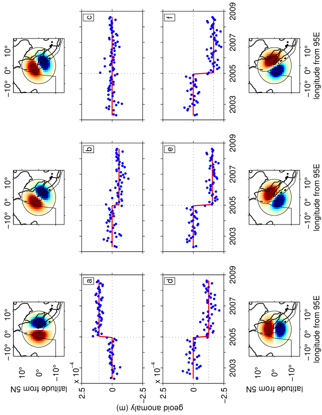
Figure 5: Orientation selectivity of the Slepian basis functions and the signal from the 12/26/2004 Sumatra-Andaman earthquake. The ‘Level-2’ time-variable gravity spherical harmonic coefficients from the Gravity Recovery And Climate Experiment[23] (GRACE) were transformed via eq. (33) to the expansion coefficients in a circularly symmetric Slepian basis of colatitudinal radius $\Theta=10^{\circ}$ and of bandwidth $L=60$, centered on the northwestern tip of the island of Sumatra, $\theta_{0}=85^{\circ}$ and $\phi_{0}=95^{\circ}$. A linear trend, annual and semiannual variations were removed prior to display. The monthly varying contributions from the $m=\pm 1$ best-concentrated ($\alpha=1$) basis functions are shown after rotation of the basis over the angles $\omega=0^{\circ},-30^{\circ}$ and $-50^{\circ}$, respectively. The final rotation projects almost all of the energy of the signal onto a single component. By this measure, the best-fitting estimate of the overall strike of the earthquake is N$40^{\circ}$W, which is in good agreement with independent seismological observations of this complex rupture[35].

Figure 5 applies this procedure to the time-variable gravity field as seen by GRACE for the Slepian basis of colatitudinal radius $\Theta=10^{\circ}$ and bandwidth $L=60$ centered at $\theta_{0}=85^{\circ}$ and $\phi_{0}=95^{\circ}$ and for varying rotations $\omega$. The gravitational-potential perturbation due to the 2004 Sumatra-Andaman earthquake is a clearly visible step in the time series of the expansion coefficients belonging to the $\alpha=1$ best concentrated $m=\pm 1$ Slepian functions, expressed as height anomalies in m above the Earth’s reference geoid. The orientation of the best-fitting fault plane can be derived from their relative contributions.

Figure 6, finally, shows our best overall estimate of the geoid perturbation due to the Sumatra-Andaman earthquake. Figure 6a–b show renderings of the signal projected onto the best-concentrated $m=0$ and $m=\pm 1$ components, respectively, of a Slepian basis with $\Theta=10^{\circ}$ and $L=60$ and varying center locations. Each pixel in Figure 6a and each arrow in Figure 6b plots the results from a different Slepian basis centered at the applicable locations $(\theta,\phi)$ shown. Figure 6c shows the results from an inversion for the statistically significant “coseismic” step-changes of the geoid due to the earthquake in each of the well-concentrated basis functions of the single Slepian basis with $\Theta=10^{\circ}$ and $L=60$ centered at $\theta_{0}=85^{\circ}$ and $\phi_{0}=95^{\circ}$, allowing also for exponential “postseismic” relaxation[25, 26]. Figure 6d shows the signal predicted independently by expanding the geoid change obtained from a combined seismological-geodynamical forward model of the earthquake rupture and the associated coseismic perturbations in a simplified Cartesian Earth model[24, 15]. More ample discussion of these models and their differences will take place in the geophysical literature.

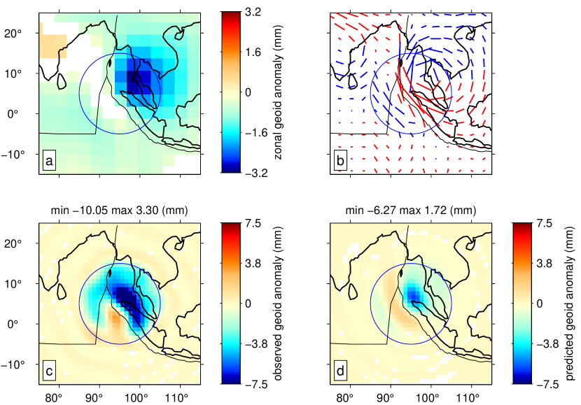
Figure 6: The signal from the 12/26/2004 Sumatra-Andaman earthquake. The analysis was carried out using identical monthly solutions from GRACE as in Figure 5 and with the same Slepian basis functions, for which $\Theta=10^{\circ}$ and $L=60$, but with their centers shifted as discussed below. The processing was identical in that a linear trend and (semi)annual variations were fitted and removed before inverting the resulting time series for the step-change due to the earthquake (the “coseismic signal”). (a) Magnitude of the zonal signal, i.e. the pointwise spatial expansion of the $m=0$ Slepian coefficients of the geoidal perturbation obtained after inversion of the time series for a step increase or decrease, using different Slepian basis sets whose centers $(\theta,\phi)$ coincide with the pixels being shown. (b) Directionality of the earthquake signal as measured by the pointwise expansion of the vectorial magnitude and direction of the $m=\pm 1$, $\alpha=1$ Slepian coefficients of the geoid change obtained by inversion of the GRACE time series. Every arrow drawn corresponds to the solution in a different Slepian basis centered at the current location, as is the case for each pixel in Figure 6a. Blue and red indicate that the positive and negative parts, respectively, of the best-fitting rotated Slepian function are to be found to the north of the arrow. (c) The best estimate of the coseismic geoid change due to the Sumatra-Andaman earthquake obtained from inversion of the Slepian expansion of the GRACE time series for a step change at the known earthquake time, also allowing for an exponential relaxation of the perturbation (the “postseismic signal”[25, 26]). The spatial expansion is complete: the single Slepian basis used was centered on $\theta_{0}=85^{\circ}$ and $\phi_{0}=95^{\circ}$. (d) Spatial rendition of the geoid change predicted independently, from seismic and geodynamical modeling of the earthquake[24, 15]. This forward model is based on several simplifying assumptions[24], and more research is needed in order to compare Figures 6c–d geophysically.

- [1] A. R. Edmonds, Angular Momentum in Quantum Mechanics, Princeton Univ. Press, Princeton, N.J., 1996.
- [2] F. A. Dahlen and J. Tromp, Theoretical Global Seismology, Princeton Univ. Press, Princeton, N. J., 1998.
- [3] F. J. Simons, F. A. Dahlen, and M. A. Wieczorek, “Spatiospectral concentration on a sphere,” SIAM Rev. 48(3), pp. 504–536, doi: 10.1137/S0036144504445765, 2006.
- [4] F. J. Simons and F. A. Dahlen, “A spatiospectral localization approach to estimating potential fields on the surface of a sphere from noisy, incomplete data taken at satellite altitudes,” in Wavelets XII, D. Van de Ville, V. K. Goyal, and M. Papadakis, eds., 6701, pp. 670117, doi: 10.1117/12.732406, Proc. SPIE, 2007.
- [5] F. J. Simons and F. A. Dahlen, “Spherical Slepian functions and the polar gap in geodesy,” Geophys. J. Int. 166, pp. 1039–1061, doi: 10.1111/j.1365–246X.2006.03065.x, 2006.
- [6] D. Slepian and H. O. Pollak, “Prolate spheroidal wave functions, Fourier analysis and uncertainty — I,” Bell Syst. Tech. J. 40(1), pp. 43–63, 1961.
- [7] H. J. Landau and H. O. Pollak, “Prolate spheroidal wave functions, Fourier analysis and uncertainty — II,” Bell Syst. Tech. J. 40(1), pp. 65–84, 1961.
- [8] D. Slepian, “Prolate spheroidal wave functions, Fourier analysis and uncertainty — IV: Extensions to many dimensions; generalized prolate spheroidal functions,” Bell Syst. Tech. J. 43(6), pp. 3009–3057, 1964.
- [9] M. A. Wieczorek and F. J. Simons, “Localized spectral analysis on the sphere,” Geophys. J. Int. 162(3), pp. 655–675, doi: 10.1111/j.1365–246X.2005.02687.x, 2005.
- [10] F. A. Dahlen and F. J. Simons, “Spectral estimation on a sphere in geophysics and cosmology,” Geophys. J. Int. 174, pp. 774–807, doi: 10.1111/j.1365–246X.2008.03854.x, 2008.
- [11] D. R. Cox and D. V. Hinkley, Theoretical Statistics, Chapman and Hall, London, UK, 1974.
- [12] J. S. Bendat and A. G. Piersol, Random data: Analysis and Measurement Procedures, John Wiley, New York, 3rd ed., 2000.
- [13] P. Xu, “Determination of surface gravity anomalies using gradiometric observables,” Geophys. J. Int. 110, pp. 321–332, 1992.
- [14] N. Sneeuw and M. van Gelderen, “The polar gap,” in Geodetic boundary value problems in view of the one centimeter geoid, F. Sansò and R. Rummel, eds., Lecture Notes in Earth Sciences 65, pp. 559–568, Springer, Berlin, 1997.
- [15] S.-C. Han and F. J. Simons, “Spatiospectral localization of global geopotential fields from the Gravity Recovery and Climate Experiment GRACE reveals the coseismic gravity change owing to the 2004 Sumatra-Andaman earthquake,” J. Geophys. Res. 113, pp. B01405, doi: 10.1029/2007JB004927, 2008.
- [16] W. M. Kaula, “Theory of statistical analysis of data distributed over a sphere,” Rev. Geophys. 5(1), pp. 83–107, 1967.
- [17] A. Albertella, F. Sansò, and N. Sneeuw, “Band-limited functions on a bounded spherical domain: the Slepian problem on the sphere,” J. Geodesy 73, pp. 436–447, 1999.
- [18] R. Pail, G. Plank, and W.-D. Schuh, “Spatially restricted data distributions on the sphere: the method of orthonormalized functions and applications,” J. Geodesy 75, pp. 44–56, 2001.
- [19] M. van Gelderen and R. Koop, “The use of degree variances in satellite gradiometry,” J. Geodesy 71, pp. 337–343, 1997.
- [20] S. Maus, M. Rother, C. Stolle, W. Mai, S. Choi, H. Lühr, D. Cooke, and C. Roth, “Third generation of the Potsdam Magnetic Model of the Earth (POMME),” Geochem. Geophys. Geosys. 7, pp. Q07008, doi: 10.1029/2006GC001269, 2006.
- [21] D. Gubbins and E. Herrero-Bervera, eds., Encyclopedia of Geomagnetism and Paleomagnetism, Springer, Dordrecht, Neth., 2007.
- [22] B. F. Chao and R. S. Gross, “Changes in the Earth’s rotation and low-degree gravitational field induced by earthquakes,” Geophys. J. Int. 91, pp. 569–596, 1987.
- [23] B. D. Tapley, S. Bettadpur, J. C. Ries, P. F. Thompson, and M. M. Watkins, “GRACE measurements of mass variability in the Earth system,” Science 305(5683), pp. 503–505, doi: 10.1126/science.1099192, 2004.
- [24] S.-C. Han, C. K. Shum, M. Bevis, C. Ji, and C.-Y. Kuo, “Crustal dilatation observed by GRACE after the 2004 Sumatra-Andaman earthquake,” Science 313, pp. 658–662, doi: 10.1126/science.1128661, 2006.
- [25] S.-C. Han, J. Sauber, S. B. Luthcke, C. Ji, and F. F. Pollitz, “Implications of postseismic gravity change following the great 2004 Sumatra-Andaman earthquake from the regional harmonic analysis of GRACE inter-satellite tracking data,” J. Geophys. Res. 113, pp. B11413, doi: 10.1029/2008JB005705, 2008.
- [26] C. de Linage, L. Rivera, J. Hinderer, J.-P. Boy, Y. Rogister, S. Lambotte, and R. Biancale, “Separation of coseismic and postseismic gravity changes for the 2004 Sumatra-Andaman earthquake from 4.6 years of GRACE observations and modeling of the coseismic change by normal-modes summation,” Geophys. J. Int. 176, pp. 695–714, doi: 10.1111/j.1365–246X.2008.04025.x, 2009.
- [27] A. M. Dziewoński and D. L. Anderson, “Preliminary Reference Earth Model,” Phys. Earth Planet. Inter. 25, pp. 297–356, 1981.
- [28] T. Nissen-Meyer, F. A. Dahlen, and A. Fournier, “Spherical-earth Fréchet sensitivity kernels,” Geophys. J. Int. 168(3), pp. 1051–1066, doi: 10.1111/j.1365–246X.2006.03123.x, 2007.
- [29] S.-C. Han and P. Ditmar, “Localized spectral analysis of global satellite gravity fields for recovering time-variable mass redistributions,” J. Geodesy 82(7), pp. 423–430, doi: 10.1007/s00190–007–0194–5, 2007.
- [30] S.-C. Han, “Improved regional gravity fields on the Moon from Lunar Prospector tracking data by means of localized spherical harmonic functions,” J. Geophys. Res. 113, pp. E11012, doi:10.1029/2008JE003166, 2008.
- [31] T. Risbo, “Fourier transform summation of Legendre series and D-functions,” J. Geodesy 70(7), pp. 383–396, 1996.
- [32] C. H. Choi, J. Ivanic, M. S. Gordon, and K. Ruedenberg, “Rapid and stable determination of rotation matrices between spherical harmonics by direct recursion,” J. Chem. Phys. 111(19), pp. 8825–8831, 1999.
- [33] B. D. Wandelt and K. M. Górski, “Fast convolution on the sphere,” Phys. Rev. D 63(12), p. 123002, 2001.
- [34] J. D. McEwen, M. P. Hobson, D. J. Mortlock, and A. N. Lasenby, “Fast directional continuous spherical wavelet transform algorithms,” IEEE Trans. Signal Process. 55(2), pp. 520–529, 2007.
- [35] T. Lay, H. Kanamori, C. J. Ammon, M. Nettles, S. N. Ward, R. C. Aster, S. L. Beck, S. L. Bilek, M. R. Brudzinski, R. Butler, H. R. DeShon, G. Ekström, K. Satake, and S. Sipkin, “The Great Sumatra-Andaman earthquake of 26 December 2004,” Science 308(5725), pp. 1127–1133, 2005.