Analysis of galaxy SEDs from far-UV to far-IR with CIGALE: Studying a SINGS test sample

Abstract

Aims. Photometric data of galaxies covering the rest-frame wavelength range from far-UV to far-IR make it possible to derive galaxy properties with a high reliability by fitting the attenuated stellar emission and the related dust emission at the same time.

Methods. For this purpose we wrote the code CIGALE (Code Investigating GALaxy Emission) that uses model spectra composed of the Maraston (or PEGASE) stellar population models, synthetic attenuation functions based on a modified Calzetti law, spectral line templates, the Dale & Helou dust emission models, and optional spectral templates of obscured AGN. Depending on the input redshifts, filter fluxes are computed for the model set and compared to the galaxy photometry by carrying out a Bayesian-like analysis. CIGALE was tested by analysing 39 nearby galaxies selected from SINGS. The reliability of the different model parameters was evaluated by studying the resulting expectation values and their standard deviations in relation to the input model grid. Moreover, the influence of the filter set and the quality of photometric data on the code results was estimated.

Results. For up to 17 filters with effective wavelengths between $0.15$ and $160$ $\mu$m, we find robust results for the mass, star formation rate, effective age of the stellar population at 4000 Å, bolometric luminosity, luminosity absorbed by dust, and attenuation in the far-UV. Details of the star formation history (excepting the burst fraction) and the shape of the attenuation curve are difficult to investigate with the available broad-band UV and optical photometric data. A study of the mutual relations between the reliable properties confirms the dependence of star formation activity on morphology in the local Universe and indicates a significant drop in this activity at about $10^{11}$ M_⊙ towards higher total stellar masses. The dustiest galaxies in the SINGS sample are present in the same mass range. On the other hand, the far-UV attenuation of our sample galaxies does not appear to show a significant dependence on star formation activity.

Conclusions. The results for our SINGS test sample demonstrate that CIGALE can be a valuable tool for studying basic properties of galaxies in the near and distant Universe if UV-to-IR data are available.

1 Introduction

Apart from dark matter, galaxies consist of stars, gas, and dust. Stars produce the radiation that allows us to observe galaxies in a wide wavelength range. Interstellar gas mainly modifies the spectral energy distributions (SEDs) of galaxies by additional line emission or absorption. Finally, interstellar dust affects galaxy SEDs by extinction, i.e. absorption and scattering of stellar radiation, especially in the UV and optical and re-emission of the absorbed energy in the IR. The dust-induced energy conversion makes it difficult to study basic properties related to the stellar populations like the star formation rate (SFR), since a good knowledge of the galaxy SEDs over a wide wavelength range is necessary to evaluate the effect of dust.

In the past, the availability of IR galaxy data (IRAS and ISO) was mainly restricted to the nearby Universe. Hence, most low-to-high-redshift galaxies could be observed in the rest-frame UV to near-IR only. Since the total amount of dust emission in the IR could not be used to determine the amount of attenuation of the stellar continuum in the observed wavelength ranges, in particular, studies of broad-band SEDs suffered from difficulties to disentangle age, metallicity, and dust effects. The lack of information made it necessary to assume a typical shape of the attenuation law (Calzetti et al. CAL94 (1994), CAL00 (2000)) and to apply simple recipes in the UV or optical to estimate the amount of attenuation. Possible variations in the galaxy dust properties could not be considered in this way, which caused high uncertainties in parameters such as the SFR. However, in view of many high-quality IR data collected by Spitzer, it is now possible to study SEDs of large galaxy samples up to high redshifts in a wide wavelength range, which allows us to better understand dust effects.

In face of the complex SEDs of galaxies consisting of emission from different stellar populations which is modified by interstellar gas and dust in a complicated way, it is clear that the derivation of galaxy properties needs a realistic modelling of galaxy SEDs. For the stellar populations those models were produced by, e.g., Fioc & Rocca-Volmerange (FIO97 (1997)), Bruzual & Charlot (BRU03 (2003)), and Maraston (MARA05 (2005)). Dust attenuation curves were either derived by studying the SEDs of nearby star-forming galaxies (Calzetti et al. CAL94 (1994), CAL00 (2000)) or by more theoretical radiative transfer models (e.g., Witt & Gordon WIT00 (2000)). The emission of dust grains in the IR and polycyclic aromatic hydrocarbons (PAHs; see Peeters et al. PEE04 (2004) and references therein) in the mid-IR was described by templates of Chary & Elbaz (CHAR01 (2001)), Dale & Helou (DAL02 (2002)), Lagache et al. (LAG03 (2003), LAG04 (2004)), and Siebenmorgen & Krügel (SIE07 (2007)). Models that also include stellar emission and dust attenuation at shorter wavelengths were published by, e.g., Silva et al. (SIL98 (1998)), Dopita et al. (DOP05 (2005)), and da Cunha et al. (CUN08 (2008)). The former also consider the evolution of dust properties dependent on the age of the stellar population. Sophisticated fitting codes of galaxy SEDs mainly focus on the derivation of redshifts and relatively robust galaxy properties like masses (e.g., Bolzonella et al. BOL00 (2000); Feldmann et al. FEL06 (2006); Walcher et al. WAL08 (2008)). Models for the IR are usually not included.

The above collection of publications on the modelling of galaxy SEDs shows that the comparison of data and models is an important tool for studying the physical properties of galaxies. However, details of the listed models like galaxy types, wavelength regimes, and characteristic parameters can differ a lot. On the other hand, the different astronomical questions and the available data sets require suitable models. Finally, optimised routines are necessary in order to derive the characteristic galaxy properties under investigation from the comparison of data and models.

Hence, we feel that an observer-friendly fitting code for star-forming galaxies at different (given) redshifts is still missing which especially provides star formation histories, dust attenuation properties, and masses and uses photometric data covering the rest-frame UV to IR to constrain these properties. In other words, we are interested in a code that calculates the effect of dust on galaxy SEDs in a consistent way in order to obtain properties (such as the SFR or the effective age of the stellar populations) which are important for understanding the evolution of galaxies. Based on a procedure described in Burgarella et al. (BUR05 (2005)), we have developed a code that derives galaxy properties by means of a Bayesian-like analysis. In Sect. 2 we describe the models used and the fitting procedure. In Sect. 3 we test the code for nearby galaxies selected from the SINGS sample (Kennicutt et al. KEN03 (2003)) for which good photometric data from the UV to the IR are available. Finally, the resulting findings concerning the applicability and effectivity of the code are discussed in Sect. 4.

2 The code

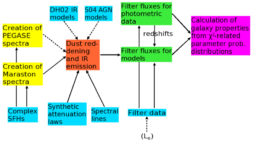
Figure 1: Flow chart of CIGALE. The different programme modules and the corresponding parameter and template inputs are shown from the left to the right. The alternative (and less preferred) use of the PEGASE models is marked by a dashed arrow. The other dashed arrows refer to the option to take either IR photometry directly (consideration of Dale & Helou and possibly Siebenmorgen et al. models) or externally estimated IR luminosities for considering the IR regime. The presented flow chart assumes that the object redshifts are taken from the photometric input catalogue.

Our programme package CIGALE (Code Investigating GALaxy Emission) is characterised by a series of modules which are fed by spectra and parameter files. A flow chart of the code is shown in Fig. 1. The general idea is to build stellar population models first. Secondly, the dust is considered by reddening the stellar SEDs and re-emitting the absorbed energy in the IR. Dust emission in the IR due to non-thermal sources can also be added. Interstellar lines are taken into account as corrections of the dust-affected SEDs. Redshift-dependent filter fluxes of the entire model set are, then, calculated for a direct comparison to the input object data. Finally, depending on the $\chi^{2}$ for the best-fit models of a set of bins in the parameter space, probability distributions as a function of the parameter value are calculated and used to derive weighted galaxy properties. Before we discuss this Bayesian-like analysis and the interpretation of its results in more detail in Sect. 2.2 and 2.3, we start with a description of the models used in Sect. 2.1.

2.1 Models

For CIGALE we take models indicating the net emission from a galaxy in the wavelength range from far-UV to far-IR. This means stellar emission, absorption and emission by dust, and at least the strongest interstellar absorption and emission lines have to be considered.

2.1.1 Stars

Concerning the stellar SEDs we have decided to focus on the models of Maraston (MARA05 (2005)), since they consider the thermally pulsating asymptotic giant branch (TP-AGB) stars in a realistic way. These stars are bright intermediate-age stars of $0.2$ to 1–2 Gyr which mostly contribute from red optical to near-IR wavelengths. Therefore, they are particular important for a reliable stellar mass determination, but star-formation-related parameters are also affected. The insufficient consideration of TP-AGB stars in older but widespread models of Bruzual & Charlot (BRU03 (2003)) and Fioc & Rocca-Volmerange (FIO97 (1997); PEGASE) typically increases the mass by $0.2$ dex for star-forming galaxies with an important population of intermediate-age stars (Maraston et al. MARA06 (2006); Salimbeni et al. SALB09 (2009)). Therefore, CIGALE also allows PEGASE models to be used for backwards compatibility.

For the calculation of complex stellar populations (CSPs) we consider single stellar populations (SSPs) of Maraston (MARA05 (2005)) and PEGASE of different metallicity $Z$ and Salpeter (SALP55 (1955)) or Kroupa (KRO01 (2001)) initial mass function (IMF). Masses based on the Salpeter IMF are about $0.2$ dex higher than for the Kroupa IMF. The galaxy mass is normalised to 1 M_⊙ and comprises the total mass of the stars (active and dead) plus gas that originates from stellar mass loss. This means that all SSP models start with a stellar mass fraction of 100%. For a Salpeter IMF the fraction reaches about 70% at the age of the Universe. The total stellar mass is provided by the code. For obtaining CSPs the SSPs of different ages are weighted and added according to the star formation scenario chosen. We provide “box models” with constant star formation over a limited period and “$\tau$ models” with exponentially decreasing SFR, respectively. While for the former scenario and ongoing star formation the instantaneous SFR at look-back time $t^{\prime}=0$ is simply calculated by the galaxy mass divided by the age, i.e. $M_{\mathrm{gal}}/t$, the SFR of the latter scenario results in

$$\mathrm{SFR}=\frac{M_{\mathrm{gal}}}{\tau(e^{t/\tau}-1)},$$ (1)

where $\tau$ is the $e$-folding or decay time. We focus on these $\tau$ models for the rest of the paper.

CIGALE allows two CSP models to be combined. Both model components are, then, linked by their mass fraction. This scenario makes it possible to consider bursts on top of an older passive or more quiescent star-forming stellar population. Although this approach allows galaxy SEDs to be fit quite well, it is clear that this scenario can only be a rough representation of the real star formation history (SFH) of a galaxy. On the other hand, the more complex SFH scenarios are, the more SED fitting suffers from degeneracies. In view of the uncertainties in the basic stellar population model parameters, CIGALE also computes two effective parameters: the mass-weighted age

$$t_{\,\mathrm{M}}=\frac{\int_{\,0}^{\,t}t^{\prime}\mathrm{SFR}(t^{\prime})\,\mathrm{d}t^{\prime}}{\int_{\,0}^{\,t}\mathrm{SFR}(t^{\prime})\,\mathrm{d}t^{\prime}}$$ (2)

and the age $t_{\,\mathrm{D4000}}$ derived from the D4000 break (see Balogh et al. BALO99 (1999)) of the unreddened SED for a single stellar population, which shows a quasi-monotonic increase of D4000 with age (see Fig. 2). The two ages are complementary, since they trace the old mass-dominating and the young light-dominating stellar population, respectively.

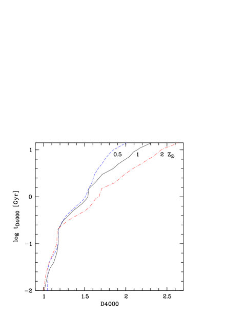
Figure 2: Relation between the age $t_{\,\mathrm{D4000}}$ and the strength of the D4000 break for Maraston (MARA05 (2005)) single stellar population models with Salpeter IMF and metallicities 0.5, 1, and 2 Z_⊙. Local, low amplitude extrema in the curves were smoothed out to avoid any ambiguities.

2.1.2 Dust attenuation

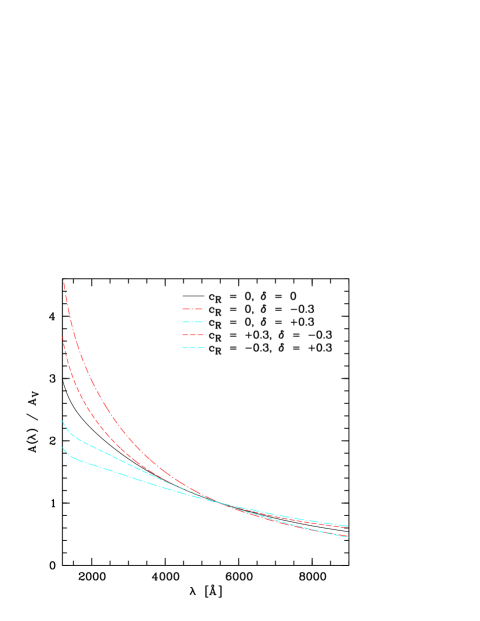
Figure 3: Illustration of synthetic attenuation laws differing in $c_{\mathrm{R}}$ and $\delta$. Apart from a pure Calzetti law ($c_{\mathrm{R}}=0$ and $\delta=0$; solid curve), Calzetti laws modified by multiplication of a power law are shown. Lower $\delta$ cause steeper slopes in the UV. In two cases the change of $R_{V}$ by the power law is compensated by $c_{\mathrm{R}}=-\delta$ (dashed curves).

The absorption and scattering of star light by dust is described by extinction curves. In the case of galaxies these laws are preferentially called attenuation curves because of the dust-induced re-scattering of radiation in direction towards the observer, which is negligible if only a single star without a circumstellar dust shell is taken into account (see Krügel KRU09 (2009)). For typical sightlines towards Milky Way stars the extinction curve is characterised by increasing extinction at shorter wavelengths, which causes a reddening of the spectra, and the so-called UV bump at about 2175 Å, which produces a broad absorption feature (e.g., Stecher STE69 (1969); Cardelli et al. CAR89 (1989); Fitzpatrick & Massa FIT07 (2007)). For typical sightlines towards the Large and Small Magellanic Cloud (LMC and SMC) the extinction curves are steeper and the UV bumps are weaker than in the Milky Way (Gordon et al. GOR03 (2003)). The most extreme curve is found for the SMC, where the 2175 Å feature is almost vanished completely. A non-existing UV bump and a moderate far-UV rise characterises the effective, average attenuation curve of nearby starburst galaxies found by Calzetti et al. (CAL94 (1994), CAL00 (2000)). However, about 30% of the UV-luminous star-forming galaxies at $1<z<2.5$ seem to exhibit a significant 2175 Å feature which can be as strong as those found in the LMC (Noll & Pierini NOL05 (2005); Noll et al. NOL07 (2007), NOL09 (2009)). Moreover, the typical width of the UV bump of these galaxies is only about 60% of those measured for characteristic Milky Way and LMC sightlines.

These observations show that a single attenuation curve as given by Calzetti et al. (CAL00 (2000)) and often used in the literature is probably insufficient to describe star-forming galaxies, in particular, at higher redshifts. Hence, we apply a more complex ansatz to describe the attenuation in our model galaxies. Since the Calzetti law seems to provide reasonable amounts of attenuation in starburst galaxies at least as an average for large samples, we take this frequently used curve as basis. For wavelengths below 1200 Å, for which the Calzetti law is not defined, we linearly extrapolate by using the value and slope at 1200 Å. This approach, which resembles the method of Bolzonella et al. (BOL00 (2000)), avoids extreme slopes at low wavelengths that are not supported by observations (Leitherer et al. LEI02 (2002)).

At first, the Calzetti law $k(\lambda)+R_{V,\,0}$ ($R_{V,\,0}=4.05\pm 0.8$) is modified by adding a UV bump which is modelled by a Lorentzian-like “Drude” profile

$$D_{\lambda_{0},\,\gamma,\,E_{\mathrm{bump}}}(\lambda)=\frac{E_{\mathrm{bump}}\,\lambda^{2}\gamma^{2}}{(\lambda^{2}-{\lambda_{0}}^{2})^{2}+\lambda^{2}\gamma^{2}},$$ (3)

where $\lambda_{0}$, $\gamma$, and $E_{\mathrm{bump}}$ are the central wavelength, width ($\approx$ FWHM), and amplitude (or maximum height), respectively (Fitzpatrick & Massa FIT90 (1990), FIT07 (2007); Noll et al. NOL09 (2009)). In order to produce different slopes, the modified Calzetti law is multiplied by a power law $(\lambda/\lambda_{V})^{\,\delta}$, where $\lambda_{V}=5500$ Å is the reference wavelength of the $V$ filter. This choice allows the slope to be changed without altering the scaling parameter visual attenuation $A_{V}$. Slopes $\delta>0$ represent flatter slopes than the Calzetti law, while $\delta=0$ exactly reproduces this basic curve if no bump is considered (see Fig. 3). If the resulting curve gives a negative attenuation correction, which even happens for a pure Calzetti law in the near-IR, no correction is applied. Since $\delta\neq 0$ causes a change in the original scaling parameter of the Calzetti attenuation curve $E_{B-V}$, the real $R_{V}=A_{V}/E_{B-V}$ differs from the value $R_{V,\,0}=4.05$ of the Calzetti law. In order to compensate for this effect and to have more freedom in the choice of this constant, the attenuation law is multiplied by the factor $(1-a_{\mathrm{R}}\,c_{\mathrm{R}})/R_{V,\,0}$. For $a_{\mathrm{R}}=1.12$ this term guarantees roughly constant $R_{V}$ if $c_{\mathrm{R}}+\delta=\mathrm{const}$ (see Fig. 3). For reasonable slope corrections $-0.3<\delta<0.3$ the real $R_{V}$ changes by about +1% or less. In summary, the dust attenuation in magnitudes as function of wavelength is

$$A(\lambda)=A_{V}\Big{[}(k(\lambda)+D_{\lambda_{0},\,\gamma,\,E_{\mathrm{bump}}}(\lambda))\frac{1-1.12\,c_{\mathrm{R}}}{4.05}+1\Big{]}\Big{(}\frac{\lambda}{5500\,\mathring{\mathrm{A}}}\Big{)}^{\delta}.$$ (4)

The attenuation correction is applied to both possible stellar population components (see Sect. 2.1.1) individually by allowing for different $A_{V}$. In practice, the visual attenuation of the young $\tau$ model $A_{V,\,\mathrm{ySP}}$ and a reduction factor of the attenuation for the old $\tau$ model $f_{\mathrm{att}}$ are used. This simple procedure takes into account that stars of different age can be affected by different amounts of dust (Silva et al. SIL98 (1998); Pierini et al. PIE04 (2004); Panuzzo et al. PAN07 (2007); Noll et al. NOL07 (2007)).

In view of the complexity of the attenuation curves and the dependence of the total attenuation on the SFH due to the introduction of $f_{\mathrm{att}}$, we characterise the effective obscuration of the stellar radiation by two additional parameters that are derived from the final model SEDs. $A_{\mathrm{FUV}}$ and $A_{V}$ are defined as the effective attenuation factors in magnitudes at $1500\pm 100$ Å and $5500\pm 100$ Å, respectively. Both parameters are complementary. While $A_{\mathrm{FUV}}$ probes the dust obscuration of the young stellar population only, $A_{V}$ also traces the attenuation of older and cooler stars. The latter parameter equals $A_{V,\,\mathrm{ySP}}$ if only one $\tau$ model is used to describe the SFH of a galaxy.

2.1.3 Dust emission

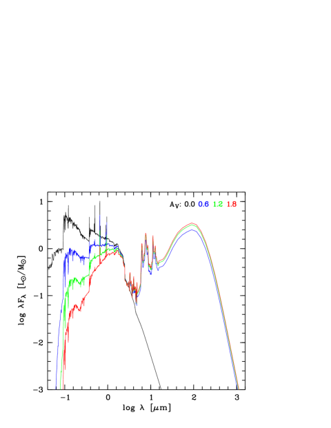
Figure 4: Illustration of a set of complete models differing in $A_{V}$ (see legend). The higher $A_{V}$ is, the lower the flux in the UV and the higher the flux in the IR is. All models are characterised by solar metallicity, $\tau=10$ Gyr, $t=1$ Gyr, Calzetti law (i.e. $c_{\mathrm{R}}=0$ and $\delta=0$), an LMC-like UV bump, no AGN contamination, and $\alpha=2.0$.

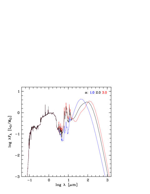
Figure 5: Illustration of a set of complete models differing in $\alpha$ (see legend). The higher $\alpha$ is, the larger the peak wavelength of the dust emission is. All models are characterised by solar metallicity, $\tau=10$ Gyr, $t=1$ Gyr, Calzetti law (i.e. $c_{\mathrm{R}}=0$ and $\delta=0$), an LMC-like UV bump, no AGN contamination, and $A_{V}=1.2$ mag.

Dust re-radiates energy predominantly absorbed in the UV and optical at relatively long, mid-IR to sub-mm wavelengths. In the far-IR dust emission is characterised by continuum radiation that originates from dust grains in thermal equilibrium. The wavelength distribution of the emission depends on grain temperature, i.e. longer wavelengths indicate lower temperatures. In the mid-IR the continuum radiation of star-forming galaxies is mainly caused by stochastically-heated very small grains (see, e.g., da Cunha et al. CUN08 (2008) and references therein). This emission is superimposed by prominent broad emission features of polycyclic aromatic hydrocarbon (PAH) molecules (see Puget & Léger PUG89 (1989); Sturm et al. STU00 (2000); Draine DRA03 (2003); Peeters et al. PEE04 (2004)). In contrast, mid-IR spectra dominated by hot dust continuum emission and lacking significant PAH emission are usually related to active galactic nuclei (AGN).

The IR properties of star-forming galaxies can be described by physically motivated multi-parameter models (e.g., Dopita et al. DOP05 (2005); Siebenmorgen & Krügel SIE07 (2007); da Cunha et al. CUN08 (2008)). However, since the IR data of galaxies at higher redshifts are usually quite sparse, we have decided to rely on semi-empirical, one-parameter models (Chary & Elbaz CHAR01 (2001), Dale & Helou DAL02 (2002), Lagache et al. LAG03 (2003), LAG04 (2004)). For CIGALE we take the 64 templates of Dale & Helou (DAL02 (2002)), which are parametrised by the power law slope of the dust mass distribution over heating intensity $\alpha$. For higher $\alpha$ the contribution of relatively quiescent galactic regions characterised by weak radiation fields becomes more important and the dust emission peaks at longer wavelengths (see Dale et al. DAL01 (2001)). The PAH emission pattern of the Dale & Helou (DAL02 (2002)) models shows only little variation. This agrees with the observations as long as the IR emission is not significantly affected by an AGN (e.g., Peeters et al. PEE04 (2004)). As for the Chary & Elbaz (CHAR01 (2001)) and Lagache et al. (LAG03 (2003)) models, a characteristic IR luminosity $L_{\mathrm{IR}}$ can be assigned to each Dale & Helou (DAL02 (2002)) template. Those calibrations for luminosity-dependent IR SEDs of the Dale & Helou models are available from Chapman et al. (CHAP03 (2003)) and Marcillac et al. (MARC06 (2006)). Since individual galaxies can significantly differ from these relations for sample averages, we do not directly use them for CIGALE. However, they can be taken to adapt the $\alpha$ parameter space for the kind of objects investigated.

The semi-empirical Dale & Helou templates include stellar emission in the near-IR range and below (see Dale et al. DAL01 (2001)). In order to combine them with stellar population models the stellar contribution needs to be subtracted. Therefore, we scaled a 5 Gyr-old passively-evolving Maraston model to the flux at $2.5-3$ $\mu$m in the different Dale & Helou models to remove the stellar emission. For wavelengths below $2.5$ $\mu$m we set the flux in the IR models to zero, in any case. The flux reduction drops below 50% at about 5 $\mu$m. The choice of the stellar population model is not critical, since the slope of the stellar continuum at these long wavelengths shows only little variation for different SFHs.

The IR templates are linked to the attenuated stellar population models by the dust luminosity $L_{\mathrm{dust}}$, i.e. the luminosity “absorbed” by the dust and re-emitted in the IR. Hence, the scaling of the Dale & Helou templates is not a free parameter. The change of the luminosity transfer with increasing $A_{V}$ for a fixed attenuation law is illustrated in Fig. 4. On the other hand, Fig. 5 demonstrates for fixed $L_{\mathrm{dust}}$ the change in the shape of the IR SED if the only IR-specific parameter $\alpha$ is modified.

The equality between the dust-absorbed and dust-emitted luminosity can be violated by dust emission caused by a non-thermal source. In particular, highly dust-enshrouded AGN represent a problem, since they are difficult to identify in the UV and optical. Consequently, galaxies with such an AGN contribution look like normal star-forming galaxies in the far-UV-to-far-IR wavelength range excepting a warm/hot dust emission in the IR. Therefore, we allow for an additional IR dust emission component which is not balanced by dust absorption of stellar emission at shorter wavelengths.

Siebenmorgen et al. (2004a , 2004b ) provide almost 1500 AGN models differing in the luminosity of the non-thermal source, the outer radius of a spherical dust cloud covering the AGN, and the amount of attenuation in the visual caused by the cloud. In principle, all models can be fed into CIGALE. Focusing on SEDs providing PAH-free mid-IR emission, the number of suitable models significantly decreases, however. As reference model we take $L=10^{12}$ L_⊙, $R=125$ pc, and $A_{V}=32$ mag. Using this or similar models allows us to disentangle IR dust emission components caused by stellar and AGN radiation, respectively, since the AGN-related component peaks at significantly shorter wavelengths than the stellar one. Admittedly, the real SEDs of obscured AGN could significantly deviate from our preferred model. However, this is almost impossible to test with broad-band photometric data only.

2.1.4 Gas

Strong spectral lines or blends can easily change filter-averaged fluxes by 10% or more. Therefore, spectral features need to be considered to avoid systematic deviations in the spectra. The crucial features are nebular emission lines of, e.g., H I, [O II], and [O III] in the optical and interstellar absorption lines of different ions in the UV. The UV is also affected by stellar wind lines like C IV and nebular emission, i.e. essentially the strongly-varying Ly$\alpha$ line. The narrow nebular emission lines in the IR are not explicitly considered, since we assume that they already contribute to the low-resolution semi-empirical templates of Dale & Helou (DAL02 (2002)).

The spectral line correction is performed by using empirical line templates. We have taken the Kinney et al. (KIN96 (1996)) starburst spectra to derive two optical emission line templates mainly differing in the strength of the oxygen lines. For the UV we have derived two line templates from composites of high-redshift galaxies of Noll et al. (NOL04 (2004)), since their UV spectra have a better quality than those of Kinney et al. (KIN96 (1996)). The UV line templates include all lines between Lyman limit and 3000 Å excepting those which are already present in the stellar population models. The selection of the optical and UV templates depends on the flux ratio of the wavelength ranges $1420-1490$ Å and $3400-3600$ Å in the attenuated stellar population models in order to reproduce the change of line strengths with UV continuum reddening in star-forming galaxies. The best agreement with the observed spectra is achieved if for ratios $\geq 3.7$ the templates with strong emission and weak absorption features are taken. For ratios $<1.0$ and star-related $L_{\mathrm{dust}}/L_{\mathrm{bol}}<0.1$ the spectral line templates are not considered at all in order to reproduce mainly passively-evolving galaxies. Before the selected line templates are added to the models, the optical line templates are scaled to the average flux in the wavelength range $3400-3600$ Å. On the other hand, the UV line templates are, first, multiplied to the dust-attenuated models cleaned from stellar lines by interpolation. The effect of the two sets of UV and optical line templates on model spectra is visible in Fig. 4.

The described procedure for the consideration of interstellar lines in the model SEDs is, of course, relatively simple. However, it avoids systematic errors, although with significant uncertainties for individual objects with SEDs deviating from the composites analysed. A clear advantage of this phenomenological approach is certainly the avoiding of new free parameters in the code.

2.2 Fitting and parameter probability distributions

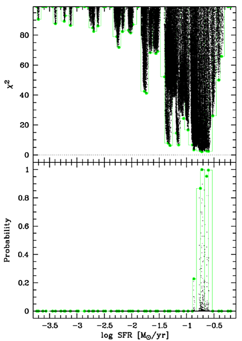
Figure 6: PDF derivation for the SFR of a test galaxy. About $7\times 10^{5}$ models are shown (small dots). The parameter space is divided into 50 bins, which are indicated by histograms. The best model of each bin is marked by a filled circle. The upper panel exhibits the $\chi^{2}$ distribution as a function of SFR. The lower panel shows the corresponding probabilities for the normalised $\chi^{2}$, i.e. $\chi^{2}-\chi^{2}_{\mathrm{best}}$. Expectation values and standard deviations for the SFR can be derived from the probability distribution of the bin-specific best-fit models.

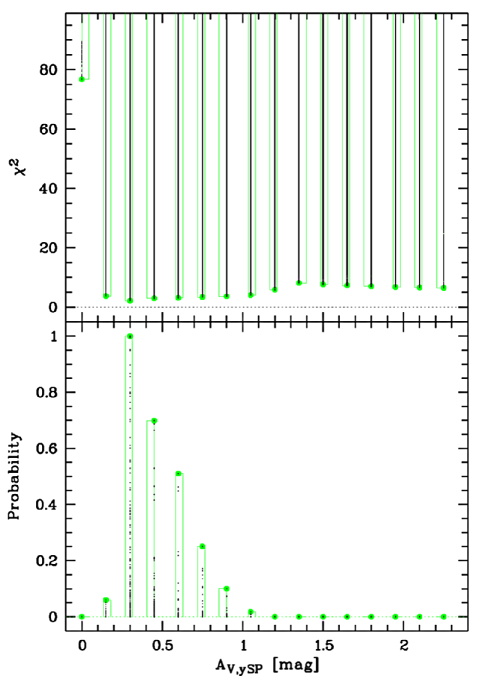
Figure 7: PDF derivation for $A_{V,\,\mathrm{ySP}}$. In this example, the discrete model $A_{V,\,\mathrm{ySP}}$ values increase in steps of $0.15$ mag. For the description of the plot see Fig. 6.

The observational input data of CIGALE are photometric filter fluxes. Hence, the filter fluxes for the entire set of models are derived for the known redshifts of the objects given. The final models taken also include a correction of the redshift-dependent absorption of the intergalactic medium (IGM) shortwards of Ly$\alpha$. Here we take the more recent algorithm of Meiksin (MEI06 (2006)) instead of the more frequently used corrections of Madau (MAD95 (1995)).

For sparse IR data it is possible to provide an externally computed IR luminosity to the code instead of using the IR filters directly. For example, the Dale & Helou (DAL02 (2002)) models can be used in combination with the calibrations of Chapman et al. (CHAP03 (2003)) and Marcillac et al. (MARC06 (2006)) to derive typical $L_{\mathrm{IR}}$ from MIPS 24 $\mu$m flux densities. In this case, $L_{\mathrm{IR}}$ is converted into flux units for an artificial filter centred at 100 $\mu$m. This is, then, compared to the dust luminosity $L_{\mathrm{dust}}$ derived for each model converted to a filter flux as well. In order to save computing time no IR models need to be considered in this case.

The comparison of model and noise-affected object photometry, i.e. of $f_{\mathrm{mod},i}$ (per $M_{\odot}$) and $f_{\mathrm{obs},i}$ for $k$ filters, is carried out for each model by the minimisation of

$$\chi^{2}(M_{\mathrm{gal}})=\sum_{i=1}^{k}\frac{(M_{\mathrm{gal}}f_{\mathrm{mod},i}-f_{\mathrm{obs},i})^{2}}{\sigma_{\mathrm{obs},i}^{2}}$$ (5)

with the galaxy mass $M_{\mathrm{gal}}$ (in $M_{\odot}$) as a free parameter. The statistical photometric errors are considered by $\sigma_{\mathrm{obs},i}$. The resulting minimum $\chi^{2}$ of each model can be compared to determine the model showing the best $\chi^{2}$ of the entire model grid for the object SED investigated. Moreover, the model-related $\chi^{2}$ allow us to perform a more sophisticated analysis to obtain galaxy properties based on probability distribution functions (PDFs).

Probabilities for individual models are often computed using the exponential term $e^{-\chi^{2}/2}$ (e.g., Kauffmann et al. 2003a ; Salim et al. SALI07 (2007); Walcher et al. WAL08 (2008)). Then, PDFs for each parameter can be derived by calculating the probability sums of the models in given bins of the parameter space. However, the results of this ‘sum’ method depend on the model density in the parameter space. In the case of a bad choice of the input model parameter values, this can cause an unintentional bias. Although the introduction of a lower threshold probability for the consideration of models can alleviate this effect, we adopt a different approach based on the best-fit models for given bins in the parameter space and integrated probabilities, which we describe in the following. We refer to this approach as ‘max’ method. We compare the results of both methods in Sect. 3.2.2.

The likelihood of a model can be inferred from $\chi^{2}$ by integrating the corresponding probability density function from $\chi^{2}$ to infinity:

$$p(\chi^{2},n)=\int_{\chi^{2}}^{\,\infty}\frac{x^{(n/2)-1}e^{-x/2}}{2^{n/2}\,\Gamma(n/2)}\,\mathrm{d}x.$$ (6)

$\Gamma$ denotes the Gamma function and $n=k-1$ the filter-related degrees of freedom. Since the minimum $\chi^{2}$, i.e. the fit quality, can vary a lot for an object sample, we prefer to use normalised $\chi^{2}_{\mathrm{norm}}=\chi^{2}-\chi^{2}_{\mathrm{best}}$ (although not forced by the code) for computing $p$ in order to guarantee similar (and better comparable) probability distributions in the model sets for the different objects. This means that the best-fit model always has $p=1$.

For calculating the object-related expectation values and uncertainties for the different model parameters, PDFs $P(x)$ depending on the parameter value $x$ are necessary. This requires to link the $p(\chi^{2},n)$ for all $m$ models studied to the $P(x)$. We do so by introducing a fixed number $b$ of equally-sized bins for each parameter. The range of bins is delimited by the lowest and highest value of a parameter in the model set. We now derive the characteristic probability $P_{i}$ of each bin $i$ by searching the maximum $p_{j}(\chi^{2},n)$ of the models $j$ located inside the bin $i$. The prior $a_{ji}=1$ if a model $j$ belongs to the bin $i$, otherwise $a_{ji}=0$. In summary, this procedure can be written in a Bayesian-like style:

$$P_{i}(x)=\max_{j=1,...,m}(p_{j}(\chi^{2},n)\,a_{ji}).$$ (7)

The resulting PDF $P_{i}(x)$ envelops the distribution of models in the $x$–$p$ plane (see Fig. 6 for a continuum of $x$ and Fig. 7 for discrete $x$). The already mentioned advantage of this approach is that $P_{i}(x)$ does not depend on the model density as a function of $x$. Consequently, the arbitrary choice of values for a parameter can hardly change $P_{i}(x)$ as long as the covered range of $x$ is comparable.

Taking the $P_{i}(x)$ as weights for each bin, the expectation value of each parameter is given as

$$\langle x\rangle=\frac{\sum_{i=1}^{b}P_{i}x_{i}}{\sum_{i=1}^{b}P_{i}}.$$ (8)

For $x_{i}$ we directly use the parameter value of the best-fit model of each bin. It corresponds to the mean value of all models in a given bin if the number of bins is significantly higher than the number of realised parameter values, which should be the case for most model parameters. Finally, the standard deviation is derived by

$$\sigma_{x}=\sqrt{\frac{\sum_{i=1}^{b}P_{i}(x_{i}-\langle x\rangle)^{2}}{\sum_{i=1}^{b}P_{i}}}.$$ (9)

Table 1: Description of the output parameters of CIGALE

Par.	Unit	Description	Dependencies
$Z$	—	metallicity ($\mathrm{Z}_{\odot}=0.02$)	basic
$\tau_{\mathrm{oSP}}$	Gyr	$e$-folding time for	basic
		old SP model
$t_{\,\mathrm{oSP}}$	Gyr	age of old SP model	basic
$\tau_{\mathrm{ySP}}$	Gyr	$e$-folding time for	basic
		young SP model
$t_{\,\mathrm{ySP}}$	Gyr	age of young SP model	basic
$f_{\mathrm{burst}}$	—	mass fraction of	basic
		young SP model
$t_{\,\mathrm{M}}$	Gyr	mass-weighted age	dep. on SP par.
$t_{\,\mathrm{D4000}}$	Gyr	D4000-related age	dep. on SP par.
$\lambda_{0}$	Å	central wavelength of	basic
		UV bump
$\gamma$	Å	FWHM of UV bump	basic
$E_{\mathrm{bump}}$	—	amplitude of UV bump	basic
$c_{\mathrm{R}}$	—	change of $R_{V}$	basic
$\delta$	—	slope correction of	basic
		Calzetti law
$A_{V,\,\mathrm{ySP}}$	mag	$V$-band attenuation	basic
		for young SP model
$f_{\mathrm{att}}$	—	reduction of $A_{V}$	basic
		for old SP model
$A_{\mathrm{FUV}}$	mag	attenuation at 1500 Å	dep. on SP and
			attenuation par.
$A_{V}$	mag	attenuation at 5500 Å	dep. on SP and
			attenuation par.
$\alpha$	—	slope of IR model	basic
$N_{\mathrm{AGN}}$	—	number of AGN model	basic
$f_{\mathrm{AGN}}$	—	$L_{\mathrm{dust}}$ fraction of	basic
		AGN model
$N_{\mathrm{emlin}}$	—	template number for	dep. on SP and
		optical lines	attenuation par.
$N_{\mathrm{abslin}}$	—	template number for	dep. on SP and
		UV lines	attenuation par.
$M_{\mathrm{gal}}$	M⊙	galaxy mass	scaling par.
$M_{\mathrm{star}}$	M⊙	total stellar mass	dep. on SP par.
			and $M_{\mathrm{gal}}$
SFR	M⊙/yr	instantaneous SFR	dep. on SP par.
			and $M_{\mathrm{gal}}$
$L_{\mathrm{bol}}$	L⊙	bolometric luminosity	dep. on all basic
			par. and $M_{\mathrm{gal}}$
$L_{\mathrm{dust}}$	L⊙	dust luminosity	dep. on all basic
			par. and $M_{\mathrm{gal}}$

CIGALE provides results for 16 basic input parameters, the scaling parameter $M_{\mathrm{gal}}$, and 10 additional output parameters that depend on different basic model properties. A complete list is given in Table 1. Apart from mean value and error, the code outputs the parameter values of the best-fit model and the full PDFs for each parameter if desired.

2.3 Interpretation of the code results

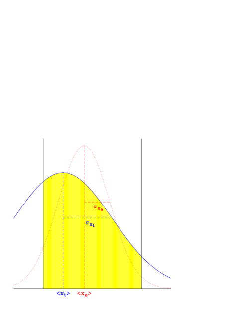
Figure 8: Illustration of the change of the mean values and standard deviations of a Gaussian PDF by the limitation of the parameter range. The cut probability distribution (filled area) indicates a mean closer to the centre of the parameter range and an error smaller than the true value.

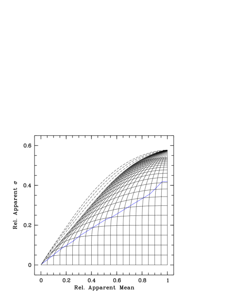
Figure 9: Deviation of the measured from the real mean values and errors for a Gaussian PDF. The axes show the apparent expectation values and standard deviations scaled to the half parameter range. The grid of solid curves indicates the true (and also scaled) mean values and errors for steps of $0.05$ from 0 to 1. Curves for constant real mean values $-0.3$, $-1$, and $-3$ outside the covered parameter range and variable real $\sigma$ are shown by dashed lines. The solid curve crossing the grid delimits the trustworthy area where the deviation between apparent and true mean values and errors is lower than 1% and 10%, respectively.

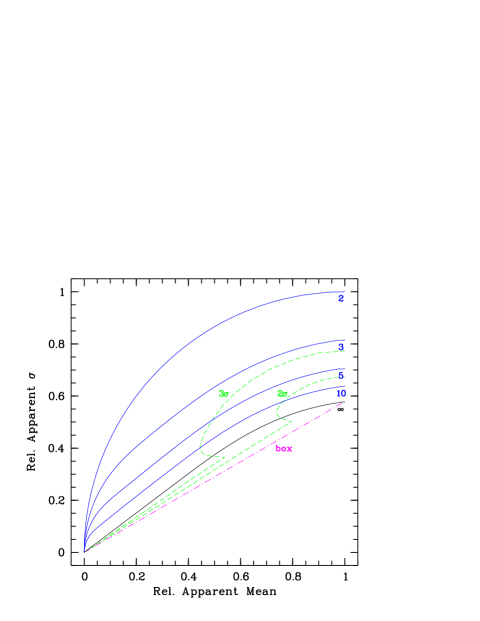
Figure 10: Curves enveloping the area allowed for data in standardised diagrams showing mean values and errors scaled to the half parameter range. The lowest solid curve corresponds to the enveloping curve of the grid shown in Fig. 9, i.e., this curve is for a Gaussian PDF with the true mean inside the parameter range and an infinite number of parameter values. The dash-dotted curve shows the same for a box-shaped distribution instead of a Gaussian. The results for double Gaussians with $2\,\sigma$ and $3\,\sigma$ separation are marked by the dashed lines. The change in the data-covered area by the reduction of the parameter input values is indicated by the solid lines labelled by the number of values.

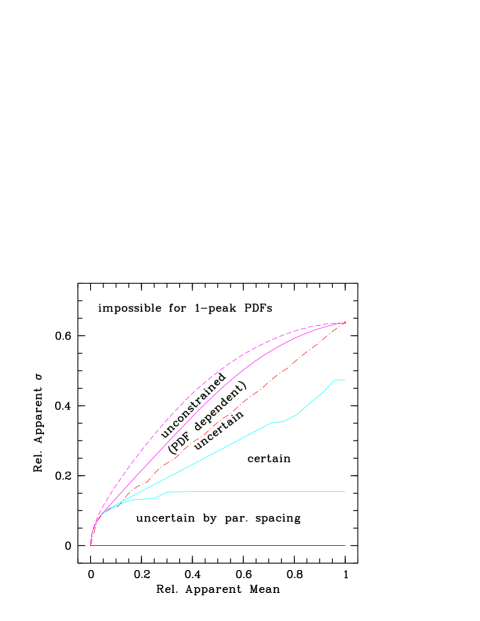
Figure 11: Normalised diagnostic plot for the interpretation of mean values and standard deviations calculated by CIGALE for 10 equally-spaced parameter values between 0 and 2, i.e. a step size of $0.22$. The outer solid/dashed curves represent the enveloping curves for a Gaussian PDF having the mean inside/outside the parameter range. The dash-dotted curve marks the enveloping curve for a box-shaped distribution. The triangular area marked by “certain” indicates for a Gaussian PDF the region of negligible difference between apparent and real mean values ($<1\%$ of the half parameter range) and errors ($<10\%$). For a box-shaped PDF this area would extend to higher $\sigma$ and be delimited by the corresponding enveloping curve. For applying the diagram to real data, the right part of the parameter range has to be complemented by the mirrored diagnostic curves and the axes have to be multiplied by half the difference of the maximum and minimum parameter values selected.

The mean values $\langle x\rangle$ and errors $\sigma_{x}$ derived by CIGALE have to be taken with care. The high complexity of the models and the limited number of photometric filters can cause that part of the parameters are not well constrained. Moreover, restrictions of computing time and hard-disc space limit and/or inherent limitations of the models used restrict the range and number of possible values for each parameter which can be investigated by the code. Since good a-priori estimates of the PDF of a parameter are rare, the selected model grid may fail to cover the entire set of parameter values consistent with the data. In this case the calculated average is probably misplaced and the errors are too small (see Fig. 8). Therefore, we study the uncertainty and reliability of the results of CIGALE by means of simulations for different PDFs for different sets of parameter values.

At first, we consider a Gaussian PDF for an infinite number of values. By changing the position and width of the Gaussian in a fixed parameter range of normalised width 2, we obtain the relation between apparent and true mean values and errors as presented in Fig. 9. For the area below the intersecting solid curve the regular grid in steps of $0.05$ does not change significantly, i.e. $\Delta\langle x\rangle<0.01$ and $\Delta\sigma_{x}<0.1$. For the centre of the Gaussian closer to the margin of the covered range and higher widths of the Gaussian the differences between true and apparent expectation values and standard deviations increase more and more until a curve that delimits the permitted area is reached. Close to this enveloping curve the corrections are enormous and highly uncertain because of the high density of curves. We can therefore divide the area of a standardised diagnostic diagram in three sub-areas which characterise reliable, uncertain/unreliable, and impossible results.

For data points that are not too close to the enveloping curve, the diagram could, in principle, be used to recover the true mean values and errors. However, the real situation is more complicated, since PDFs do not need to be Gaussian (see, e.g., Figs. 6 and 7). Fig. 10 shows enveloping curves (for the true mean located inside the parameter range) for different shapes of the probability distribution. For a box-shaped distribution the possible errors are generally lower. On the other hand, double-peak profiles can cause relatively high apparent errors close to the centre of the parameter range. In this case, the true mean can be located in the other half of the parameter range, which is not possible for the single-peak PDFs discussed before.

Finally, Fig. 10 illustrates that a finite number of parameter input values causes an increase of the errors. In the most extreme case of two values, only the margins of the parameter range are covered by data points, which produces significantly higher standard deviations than for a smooth PDF. In contrast to uncertainties in the shape of the probability distribution that impede a detailed diagnostics and correction, changes in the mean values and errors by the reduction of parameter values can be recovered and considered for the interpretation of the code results. Additional uncorrectable deviations are only caused if the true error is smaller than the difference between adjacent parameter values.

In summary, diagnostic plots with similar curves as presented in this section can be used to evaluate whether mean values and errors resulting from CIGALE are reliable, uncertain, or unreliable (implying an unconstrained parameter). Fig. 11 illustrates these different areas in a diagnostic plot similar to those used for the interpretation of the code results in Sect. 3.3.1. Only for data points in or close to the “certain” area the real PDF of a parameter can be well described by expectation value and standard deviation provided by CIGALE, otherwise the shape of the PDF has to be studied in more detail or it has to be accepted that the parameter cannot be constrained for the photometric data and model set given.

3 A test sample: SINGS

In order to establish CIGALE as a tool for studying properties of nearby and distant star-forming galaxies, it has to be tested by using a well-known reference data set. In the context of the Spitzer Infrared Nearby Galaxy Survey (SINGS; Kennicutt et al. KEN03 (2003)) high-quality photometric data were obtained in the IR regime for a sample of representative nearby galaxies. Together with the available photometric data for the other wavelength ranges (Dale et al. DAL07 (2007); Muñoz-Mateos et al. MUN09 (2009)) this data set allows us to investigate the properties of the code in detail. We describe the sample in Sect. 3.1 and discuss the analysis of the data set by means of CIGALE in Sect. 3.2. The results and a comparison to the literature are presented in Sect. 3.3.

3.1 The sample

Table 2: Properties of the SINGS test sample. Although we list the relatively conservative run B results (see Sect. 3.2.2), the given standard deviations could underestimate the real uncertainties because of the limited model grid used, model inaccuracies, and possible unconsidered photometric errors.

ID	Typea	Dist.a		$\log M_{\mathrm{star}}$		$\log\mathrm{SFR}$		$\log t_{\,\mathrm{D4000}}$b		$\log L_{\mathrm{bol}}$		$\log L_{\mathrm{dust}}$		$A_{\mathrm{FUV}}$
		[Mpc]		[M⊙]		[M⊙/yr]		[Gyr]		[L⊙]		[L⊙]		[mag]
NGC 0024	SAc	8.	2	9.65 $\pm$	0.07	-0.93 $\pm$	0.14	-0.09 $\pm$	0.23	9.47 $\pm$	0.02	8.66 $\pm$	0.05	0.59 $\pm$	0.17
NGC 0584	E4	27.	6	11.39 $\pm$	0.03	-1.10 $\pm$	0.33	0.93 $\pm$	0.07	10.92 $\pm$	0.01	8.98 $\pm$	0.15	1.41 $\pm$	0.67
NGC 0925	SABd	10.	1	10.15 $\pm$	0.12	0.07 $\pm$	0.15	-0.42 $\pm$	0.09	10.26 $\pm$	0.03	9.68 $\pm$	0.04	0.70 $\pm$	0.15
NGC 1097	SBb	16.	9	11.35 $\pm$	0.10	0.84 $\pm$	0.17	0.00 $\pm$	0.26	11.17 $\pm$	0.02	10.77 $\pm$	0.04	1.83 $\pm$	0.40
NGC 1291	SBa	9.	7	11.16 $\pm$	0.03	-0.66 $\pm$	0.27	0.85 $\pm$	0.09	10.70 $\pm$	0.01	9.37 $\pm$	0.07	1.21 $\pm$	0.59
NGC 1316	SAB0	26.	3	12.03 $\pm$	0.02	-0.14 $\pm$	0.45	0.90 $\pm$	0.08	11.56 $\pm$	0.01	10.10 $\pm$	0.06	1.59 $\pm$	0.86
NGC 1404	E1	25.	1	11.52 $\pm$	0.02	-1.01 $\pm$	0.22	0.97 $\pm$	0.02	11.04 $\pm$	0.01	8.46 $\pm$	0.10	0.48 $\pm$	0.16
NGC 1512	SBab	10.	4	10.43 $\pm$	0.08	-0.28 $\pm$	0.20	0.15 $\pm$	0.22	10.15 $\pm$	0.02	9.44 $\pm$	0.05	0.91 $\pm$	0.30
NGC 1566	SABbc	18.	0	11.05 $\pm$	0.13	0.88 $\pm$	0.18	-0.35 $\pm$	0.08	11.05 $\pm$	0.02	10.62 $\pm$	0.04	1.30 $\pm$	0.28
NGC 1705	Am	5.	8	8.51 $\pm$	0.08	-1.48 $\pm$	0.19	-0.52 $\pm$	0.03	8.73 $\pm$	0.03	7.81 $\pm$	0.04	0.23 $\pm$	0.05
NGC 2798	SBa	24.	7	10.32 $\pm$	0.11	0.68 $\pm$	0.12	-0.62 $\pm$	0.09	10.64 $\pm$	0.02	10.51 $\pm$	0.03	4.53 $\pm$	0.32
NGC 2841	SAb	9.	8	10.99 $\pm$	0.03	-0.31 $\pm$	0.24	0.60 $\pm$	0.18	10.55 $\pm$	0.01	9.66 $\pm$	0.05	1.18 $\pm$	0.40
NGC 2976	SAc	3.	5	9.48 $\pm$	0.11	-0.78 $\pm$	0.16	-0.33 $\pm$	0.07	9.39 $\pm$	0.02	8.92 $\pm$	0.05	1.45 $\pm$	0.18
NGC 3031	SAab	3.	5	11.00 $\pm$	0.04	-0.22 $\pm$	0.15	0.51 $\pm$	0.23	10.60 $\pm$	0.01	9.60 $\pm$	0.05	0.90 $\pm$	0.36
NGC 3184	SABcd	8.	6	10.28 $\pm$	0.13	0.11 $\pm$	0.15	-0.36 $\pm$	0.06	10.26 $\pm$	0.01	9.76 $\pm$	0.04	1.13 $\pm$	0.19
NGC 3190	SAap	17.	4	10.92 $\pm$	0.03	-0.85 $\pm$	0.51	0.82 $\pm$	0.12	10.46 $\pm$	0.01	9.67 $\pm$	0.05	2.06 $\pm$	0.87
NGC 3198	SBc	9.	8	10.10 $\pm$	0.12	-0.03 $\pm$	0.15	-0.34 $\pm$	0.04	10.13 $\pm$	0.01	9.60 $\pm$	0.04	0.89 $\pm$	0.17
NGC 3351	SBb	9.	3	10.66 $\pm$	0.08	-0.04 $\pm$	0.19	0.17 $\pm$	0.18	10.39 $\pm$	0.01	9.83 $\pm$	0.05	1.31 $\pm$	0.36
NGC 3521	SABbc	9.	0	11.00 $\pm$	0.04	0.43 $\pm$	0.22	-0.28 $\pm$	0.03	10.80 $\pm$	0.01	10.37 $\pm$	0.04	2.74 $\pm$	0.37
NGC 3621	SAd	6.	2	10.21 $\pm$	0.14	0.12 $\pm$	0.15	-0.40 $\pm$	0.09	10.28 $\pm$	0.02	9.88 $\pm$	0.04	1.31 $\pm$	0.26
NGC 3627	SABb	8.	9	10.95 $\pm$	0.05	0.55 $\pm$	0.22	-0.29 $\pm$	0.03	10.79 $\pm$	0.02	10.40 $\pm$	0.05	2.31 $\pm$	0.31
NGC 4536	SABbc	25.	0	11.00 $\pm$	0.14	0.96 $\pm$	0.15	-0.41 $\pm$	0.07	11.12 $\pm$	0.02	10.82 $\pm$	0.04	2.00 $\pm$	0.33
NGC 4559	SABcd	11.	6	10.27 $\pm$	0.08	0.12 $\pm$	0.08	-0.51 $\pm$	0.01	10.45 $\pm$	0.01	9.90 $\pm$	0.04	0.80 $\pm$	0.18
NGC 4569	SABab	20.	0	11.41 $\pm$	0.02	0.49 $\pm$	0.22	0.33 $\pm$	0.08	11.05 $\pm$	0.01	10.29 $\pm$	0.07	2.23 $\pm$	0.37
NGC 4579	SABb	20.	0	11.44 $\pm$	0.03	0.23 $\pm$	0.24	0.44 $\pm$	0.20	11.04 $\pm$	0.01	10.21 $\pm$	0.05	2.02 $\pm$	0.57
NGC 4594	SAa	13.	7	11.75 $\pm$	0.02	-0.47 $\pm$	0.47	0.92 $\pm$	0.05	11.27 $\pm$	0.01	9.79 $\pm$	0.06	1.60 $\pm$	0.89
NGC 4625	SABmp	9.	5	9.35 $\pm$	0.13	-0.72 $\pm$	0.11	-0.34 $\pm$	0.05	9.35 $\pm$	0.02	8.83 $\pm$	0.04	0.86 $\pm$	0.19
NGC 4631	SBd	9.	0	10.47 $\pm$	0.14	0.70 $\pm$	0.20	-0.62 $\pm$	0.08	10.76 $\pm$	0.02	10.50 $\pm$	0.04	1.49 $\pm$	0.21
NGC 4725	SABab	17.	1	11.40 $\pm$	0.04	0.35 $\pm$	0.18	0.43 $\pm$	0.18	11.01 $\pm$	0.00	10.14 $\pm$	0.04	1.12 $\pm$	0.33
NGC 4736	SAab	5.	3	10.80 $\pm$	0.07	0.07 $\pm$	0.20	0.11 $\pm$	0.23	10.52 $\pm$	0.00	9.89 $\pm$	0.04	1.54 $\pm$	0.36
NGC 4826	SAab	5.	6	10.77 $\pm$	0.02	-0.32 $\pm$	0.21	0.31 $\pm$	0.10	10.40 $\pm$	0.00	9.60 $\pm$	0.04	2.38 $\pm$	0.34
NGC 5033	SAc	13.	3	10.77 $\pm$	0.11	0.31 $\pm$	0.20	-0.27 $\pm$	0.06	10.67 $\pm$	0.01	10.30 $\pm$	0.04	1.88 $\pm$	0.29
NGC 5055	SAbc	8.	2	10.96 $\pm$	0.06	0.43 $\pm$	0.22	-0.28 $\pm$	0.02	10.78 $\pm$	0.01	10.33 $\pm$	0.04	2.22 $\pm$	0.31
NGC 5194	SABbc	8.	2	10.82 $\pm$	0.12	0.79 $\pm$	0.15	-0.44 $\pm$	0.07	10.97 $\pm$	0.02	10.62 $\pm$	0.05	1.78 $\pm$	0.29
NGC 5195	SB0p	8.	2	10.77 $\pm$	0.02	-0.12 $\pm$	0.21	0.33 $\pm$	0.08	10.41 $\pm$	0.01	9.72 $\pm$	0.05	3.36 $\pm$	0.38
NGC 5474	SAcd	6.	9	9.30 $\pm$	0.06	-0.65 $\pm$	0.14	-0.45 $\pm$	0.04	9.50 $\pm$	0.02	8.59 $\pm$	0.05	0.27 $\pm$	0.06
NGC 5713	SABbcp	26.	6	10.77 $\pm$	0.08	0.73 $\pm$	0.19	-0.53 $\pm$	0.04	10.93 $\pm$	0.01	10.71 $\pm$	0.03	2.86 $\pm$	0.33
NGC 5866	S0	12.	5	10.88 $\pm$	0.03	-0.92 $\pm$	0.54	0.78 $\pm$	0.12	10.43 $\pm$	0.00	9.30 $\pm$	0.06	2.51 $\pm$	1.18
NGC 7331	SAb	15.	7	11.39 $\pm$	0.08	0.78 $\pm$	0.20	-0.04 $\pm$	0.25	11.17 $\pm$	0.02	10.76 $\pm$	0.04	2.66 $\pm$	0.50

• see Kennicutt et al. (KEN03 (2003))

• Significant deviations of the metallicity from the solar value may affect the results for $t_{\,\mathrm{D4000}}$ (see Sect. 3.2.1).

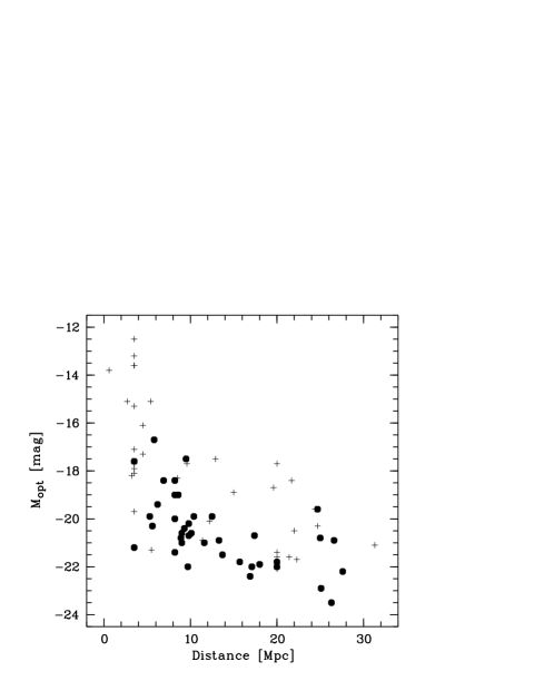
Figure 12: Optical (i.e. mainly $R$) absolute magnitudes and distances in Mpc for the SINGS galaxies (see Kennicutt et al. KEN03 (2003)). The analysed objects are indicated by filled symbols.

The full SINGS sample consists of 75 representative nearby galaxies (Kennicutt et al. KEN03 (2003)), i.e., the different morphological classes from ellipticals to irregulars have similar weights. Moreover, the galaxies are distributed over roughly equal logarithmic bins in IR luminosity. Dale et al. (DAL07 (2007), DAL08 (2008)) published UV-to-radio broad-bands SEDs for the SINGS galaxies. The listed data comprises the $FUV$ ($\sim 1500$ Å) and $NUV$ ($\sim 2300$ Å) filters of GALEX (Gil de Paz et al. GIL07 (2007)), 2MASS data for $J$, $H$, and $K_{\mathrm{s}}$ (Jarrett et al. JAR03 (2003)), and IRAC and MIPS data for the filters centred on $3.6$, $4.5$, $5.8$, $8.0$, $24$, $70$, and $160$ $\mu$m (Dale et al. DAL05 (2005)). Moreover, Dale et al. provide previously unpublished optical photometry for $B$, $V$, $R$, and $I$. However, since the optical data are erroneous, we take the improved photometry of Muñoz-Mateos et al. (MUN09 (2009)), which is based on asymptotic magnitudes that were derived from surface photometry by extrapolating the curve of growth to encompass the whole galaxy light. Apart from all non-optical Dale et al. filters up to MIPS $160$ $\mu$m, their catalogue provides photometry of the Sloan Digital Sky Survey (SDSS; Stoughton et al. STO02 (2002)) in $u^{\prime}$, $g^{\prime}$, $r^{\prime}$, $i^{\prime}$, and $z^{\prime}$ for 32 SINGS objects. Moreover, the Dale et al. (DAL07 (2007), DAL08 (2008)) optical magnitudes of 23 galaxies without SDSS photometry were recalibrated by means of the catalogue of Prugniel & Heraudeau (PRU98 (1998)), i.e., their aperture photometry was replicated on the SINGS optical images to derive zero-point corrections for each filter and each galaxy. For our sample selection we have required either the presence of SDSS photometry or at least three corrected Dale et al. filters. The latter criterion fulfil 16 of 23 objects with recovered photometry only. Three of them do not have $R$-band photometry. Finally, we only take galaxies for which all UV and IR filters are available. Our selection criteria aim at ensuring a comprehensive photometric sample of similar high quality and wavelength coverage. Considering all criteria, our final sample comprises 39 SINGS galaxies (see Table 2). Fig. 12 shows the basic properties distance and absolute magnitude (mainly $R$) as given by Kennicutt et al. (KEN03 (2003)) for our subsample compared to the full sample. The diagram indicates that dwarf galaxies are underrepresented in our sample. There are no optical magnitudes for these galaxies in the catalogue of Muñoz-Mateos et al. (MUN09 (2009)) because of recalibration problems.

3.2 Analysis

In the following we discuss the model grid that was selected to analyse our test sample of SINGS galaxies (Sect. 3.2.1). Moreover, the quality of the fitting (Sect. 3.2.2) and the influence of the filter set on the results (Sect. 3.2.3) is studied.

3.2.1 The model grid

Table 3: Selected model parameter values for the analysis of our SINGS sample

Par.	Min.	Max.	$N$
$Z$ [Z⊙]	$1.0$	$1.0$	1
$\tau_{\mathrm{oSP}}$ [Gyr]	$0.25$	$10.0$	4
$t_{\,\mathrm{oSP}}$ [Gyr]	$10.0$	$10.0$	1
$\tau_{\mathrm{ySP}}$ [Gyr]	$0.05$	$1.0$	3
$t_{\,\mathrm{ySP}}$ [Gyr]	$0.05$	$0.2$	2
$f_{\mathrm{burst}}$	$0.0001$	$0.9999$	9
$E_{\mathrm{bump}}$	$0.0$	$0.0$	1
$c_{\mathrm{R}}$	$0.0$	$0.0$	1
$\delta$	$-0.3$	$0.3$	5
$A_{V,\,\mathrm{ySP}}$	$0.0$	$2.25$	16
$f_{\mathrm{att}}$	$0.0$	$1.0$	5
$\alpha$	$1.0$	$3.0$	9
$f_{\mathrm{AGN}}$	$0.0$	$0.0$	1

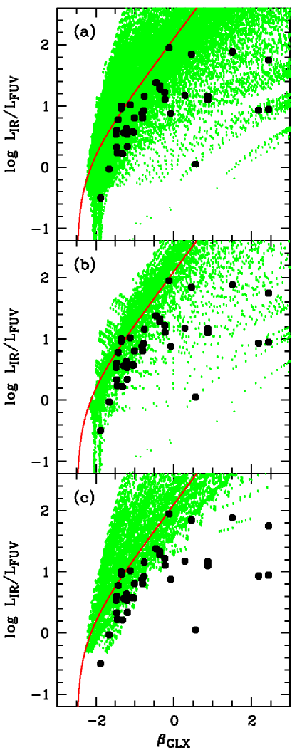
Figure 13: The IR-to-far-UV luminosity ratio $L_{\mathrm{IR}}/L_{\mathrm{FUV}}$ versus the UV continuum slope $\beta_{\mathrm{GLX}}$ for the SINGS sample. The solid curve indicates the theoretical position of starbursts in the diagram (Kong et al. KON04 (2004)). The area in the $\beta_{\mathrm{GLX}}$–$L_{\mathrm{IR}}/L_{\mathrm{FUV}}$ plane that is covered by CIGALE models is marked by small dots. Subfigure (a) shows the full model set for the parameters given in Table 3. In (b) no slope correction of the Calzetti law is considered, i.e. $\delta=0$. Finally, in (c) the stellar radiation is reddened regardless of the stellar population, i.e. $f_{\mathrm{att}}=1$.

Studying the properties of our sample of 39 SINGS galaxies by SED fitting requires a careful selection of model parameters, since the parameter space has to be restricted for computing time reasons. Table 3 shows the model grid that we have eventually used. The individual values were selected to provide (roughly) equally-sized steps in the given units or in dex for dynamical ranges larger than one order of magnitude. Only eight parameters have multiple input values, which is distinctly lower than the 15 to 17 filters available for the SINGS galaxies in our sample. The total number of models is about $7\times 10^{5}$, which can be managed quite easily on a typical PC because of a runtime of CIGALE of a few hours only.

For all stellar population models we use Maraston (MARA05 (2005)) SEDs with Salpeter IMF and solar metallicity. The latter is justified by a mean oxygen abundance $\langle 12+\log(\mathrm{O/H})\rangle=8.69$ and a scatter of $0.16$ for 23 sample galaxies listed in Calzetti et al. (CAL07 (2007)). Moreover, our sample lacks the low-metallicity dwarf galaxies present in the complete SINGS sample (see Fig. 12). However, metallicity measurements are relatively uncertain due to high-quality requirements of the observations, insufficient coverage of a galaxy in combination with abundance gradients, and, in particular, calibration problems and general limitations of the metallicity tracer (see Moustakas & Kennicutt MOU06 (2006) and references therein). Hence, we have checked the influence of the use of half and double solar metallicities on the results of the analysis of our SINGS sample. In general, the resulting properties indicate deviations within the errors and the corresponding uncertainties increase by 0 to 20% only if metallicity uncertainties are considered. The only exception is the effective age measured at 4000 Å $t_{\,\mathrm{D4000}}$, which indicates a decrease of about $0.4$ dex for a metallicity increase of a factor of 4. Consequently, the absolute values of $t_{\,\mathrm{D4000}}$ have to be taken with care due to the well-known age-metallicity degeneracy (e.g., Kodama & Arimoto KOD97 (1997)).

In CIGALE SFHs are modelled by the combination of two models with exponentially decreasing SFR (see Sect. 2.1.1). For the “old” stellar population model we take a fixed age of 10 Gyr, which should be a good compromise between the age of the Universe and the most important phase of star formation for the galaxies investigated. The $\tau$ values cover a relatively large range of values in order to account for the different kinds of SFHs possible. Due to the low effect of old stellar populations on galaxy SEDs, it is sufficient to select a few values only. For the “young” stellar population model we also take a few ages and $\tau$ only, since the variety of SEDs dominated by young stars is not very large. On the other hand, the mass fractions of both $\tau$ models are critical. Therefore, we analyse nine burst fractions $f_{\mathrm{burst}}$ covering the full range of theoretically possible values.

The obscuration of the stellar populations by dust is considered by the application of attenuation laws with different reasonable slopes (i.e. slopes not too far from the Calzetti et al. (CAL00 (2000)) law) but without a UV bump. Since the UV wavelength range of the SINGS galaxies is covered by the two GALEX filters only, details of the attenuation law are difficult to study and insignificant for most galaxy properties as test runs of CIGALE indicate for a wide range of attenuation-related parameters. Therefore, we can restrict the number of models by only taking the default value zero of the $R_{V}$-related parameter $c_{\mathrm{R}}$ and by only considering slope corrections $\delta$ between $-0.3$ and $0.3$, which result in real $R_{V}$ between $3.0$ and $5.9$ (see Sect. 2.1.2 and Fig. 3). Moreover, we fix the UV bump strength and select a value of zero. Apart from the negligible effect of the UV bump on the fit results for a wide range of strengths (cf. Noll et al. NOL09 (2009)), this choice is justified by the non-detection of a UV bump in local starburst galaxies (Calzetti et al. CAL94 (1994)), the lack of a significant 2175 Å feature in the Kinney et al. (KIN96 (1996)) characteristic UV spectra of nearby galaxies covering a large range of star formation activity, the only low-to-moderate UV bump strengths in different galaxy populations (also comprising “normal” star-forming galaxies) studied at intermediate/high redshift (Noll et al. NOL09 (2009)), and the predicted weakening of the UV bump in local spiral galaxies by radiative transfer effects (Silva et al. SIL98 (1998); Pierini et al. PIE04 (2004)).

Since the $V$-band attenuation of the young $\tau$ model $A_{V,\,\mathrm{ySP}}$ has an important effect on the (UV) SED slope and the UV-to-IR flux ratio, we choose a fine grid of values and a sufficiently high upper limit. The attenuation factor $f_{\mathrm{att}}$ indicates the fraction of $A_{V,\,\mathrm{ySP}}$ valid for the old $\tau$ model. The possibility to vary this parameter is crucial for fitting non-starburst galaxies as typically found in our SINGS sample. In Fig. 13 we show the luminosity ratio $L_{\mathrm{IR}}/L_{\mathrm{FUV}}$ and the UV continuum slope $\beta_{\mathrm{GLX}}$ of our sample galaxies. $L_{\mathrm{IR}}$ was derived from the MIPS 24, 70, and 160 $\mu$m filters as described in Dale & Helou (DAL02 (2002)). And based on GALEX $FUV$ and GALEX $FUV-NUV$, respectively, $L_{\mathrm{FUV}}$ and $\beta_{\mathrm{GLX}}$ were calculated following the recipes of Kong et al. (KON04 (2004)). The objects are located close to or below the so-called “Meurer” relation (Meurer et al. MEU99 (1999); Kong et al. KON04 (2004)). This curve is valid for starburst galaxies where the stellar content is completely obscured by a dust screen or shell. As the results of CIGALE in subfigure (c) imply, the galaxy distribution found cannot be explained by a deviation of the effective attenuation curve from the Calzetti law. Instead, subfigure (b) illustrates that an age-dependent amount of attenuation (cf. Silva et al. SIL98 (1998); Pierini et al. PIE04 (2004); Panuzzo et al. PAN07 (2007); Noll et al. NOL07 (2007)) as simulated by $f_{\mathrm{att}}$ is able to reproduce the distribution of SINGS galaxies. Then, the data points that deviate most from the starburst curve are characterised by high obscuration of a young stellar component of very low mass (low $f_{\mathrm{burst}}$) and nearly unattenuated old stellar populations. Consequently, our code is suitable to study “normal” star-forming galaxies which are usually located below the Meurer curve and are typical of the nearby Universe (see Buat et al. BUA05 (2005); Cortese et al. COR06 (2006); Dale et al. DAL07 (2007); Salim et al. SALI07 (2007)).

Dale & Helou (DAL02 (2002)) offer IR dust emission templates in the $\alpha$ range from $0.0625$ to $4.0$. Our selection covers $\alpha$ values between $1.0$ and $3.0$. The narrower range is reasonable, since $\alpha\geq 1.0$ correspond to mean IR luminosities $L_{\mathrm{IR}}\la 4\times 10^{13}$ L_⊙ according to the calibrations of Chapman et al. (CHAP03 (2003)) and Marcillac et al. (MARC06 (2006)). This is a safe limit even if the scatter in the calibrations is considered, since the SINGS sample is characterised by relatively low IR luminosities (see Kennicutt et al. KEN03 (2003)). For very high $\alpha$ values the IR SEDs become very similar for the wavelength range studied. The calibrations of Chapman et al. and Marcillac et al., which are based on the ratio of the rest-frame fluxes at 60 and 100 $\mu$m, are degenerated in this case. Therefore, it does not make sense to analyse $\alpha$ values beyond $3.0$.

Finally, we do not use the option of an AGN contamination or hot-dust contribution for the main run. Although there are several Seyfert galaxies in the sample (Kennicutt et al. KEN03 (2003)), we do not expect that the total magnitudes of the selected galaxies are significantly affected by such a contribution. Nevertheless, we have checked with a different set of models allowing for a large range of hot-dust IR contributions whether CIGALE reproduces the expected result. Indeed, the vast majority of IR SEDs is consistent with no contribution at all. Only for the early-type galaxy NGC 1404 we find a significant ($>10$%) hot-dust fraction. However, this result could also be explained by possible difficulties to fit the mixture of stellar radiation and very weak dust emission in the mid-IR of this special galaxy. Moreover, the fluxes at 70 and 160 $\mu$m have to be taken with care due to a possible contamination by a background source (see note in Table 2).

3.2.2 The fit quality

Table 4: Mean photometric errors for our SINGS test sample

Filters	Rel. errors
GALEX $FUV$, $NUV$	15%
Dale et al. $B$, $V$, $R$, $I$	16%
SDSS $u^{\prime}$, $g^{\prime}$, $r^{\prime}$, $i^{\prime}$, $z^{\prime}$	3%
2MASS $J$, $H$, $K_{\mathrm{s}}$	1%
IRAC $3.6$, $4.5$, $5.8$, $8.0$ $\mu$m	11%
MIPS $24$ $\mu$m	5%
MIPS $70$ $\mu$m	7%
MIPS $160$ $\mu$m	13%

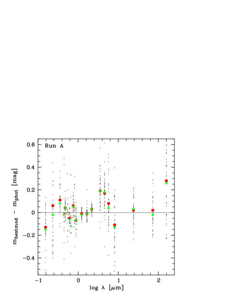
Figure 14: Ratio of the best-fit model fluxes and the measured object fluxes in mag for run A and different filters and objects. The filters are indicated by their mean wavelength. Sample-related mean and median deviations for each filter are marked by big circles and lozenges, respectively. The open symbols indicate the recalibrated optical filters of Dale et al. (DAL07 (2007)).

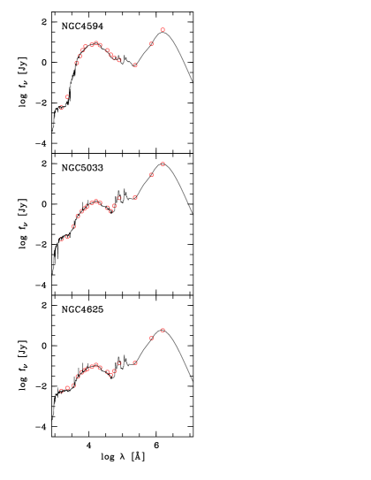
Figure 15: Illustration of three characteristic best-fit SEDs (run A) which differ in their UV-to-optical flux ratios. From top to bottom, the SEDs of NGC 4594 (Sa), NGC 5033 (Sc), and NGC 4625 (Sm) are shown. The measured photometric fluxes are marked by circles.

For the analysis of the properties of our SINGS test sample we use the total magnitudes of 21 filters and its errors reported in Muñoz-Mateos et al. (MUN09 (2009)). The typical uncertainties for the different filters are listed in Table 4. They are dominated by the instrument-related zero-point errors or uncertainties of photometric corrections and vary between 1% for the 2MASS near-IR filters and 16% for the Dale et al. (DAL07 (2007)) optical magnitudes corrected by Muñoz-Mateos et al. (MUN09 (2009)). The latter are only relevant for 15 of 39 sample galaxies for which SDSS photometry of much higher precision is not available. Since the relative photometric errors represent the weights for the different filters in the fitting process, the weights of the optical magnitudes for the two subsamples with and without SDSS photometry are quite different. Therefore, we will discuss the results of both subsamples separately in Sect. 3.3.

The large differences in the reported uncertainties for the filter fluxes obtained by different projects and instruments raises the question whether these values are really comparable. The homogeneity of the error evaluation is crucial for reliable fitting results. In particular, very low errors such as reported for the 2MASS filters are critical, since this causes hard constraints for the model set. Moreover, especially small errors are questionable, since possible systematic offsets between different filters can cause erroneous fits. Since the models are not a perfect reproduction of the nature, systematic errors are also expected for them if the fluxes of different wavelength ranges are compared. For most wavelengths we assume uncertainties in the order of 5 to 10%. Higher values are especially expected for the rest-frame wavelength range between $2.5$ and 5 $\mu$m for which the continuum is relatively uncertain due to the mixing of stellar and dust emission and fundamental uncertainties in the shape of both components. An example is the insufficient knowledge of the contribution of TP-AGB stars at these wavelengths (see Maraston MARA05 (2005)). Therefore, we study two different photometric catalogues. In the first case (‘run A’) we take the published errors (see Table 4) and in the second case (‘run B’) we increase them by adding an additional moderate 5% error in quadrature to all filter errors. This procedure allows us to investigate how the results change if additional systematic uncertainties are considered.

As a first result of CIGALE, Fig. 14 shows the deviations of the best-fit models from the object photometry in magnitudes for each filter. Since the best-fit models of both runs indicate similar photometric fluxes, we only plot the data of run A. In general, the sample-averaged deviations for the different filters are relatively small. On average, the difference is $0.07$ mag only. The worst filters are MIPS 160 $\mu$m, IRAC $3.6$ $\mu$m, and IRAC $4.5$ $\mu$m with deviations amounting to $0.28$, $0.19$, and $0.17$ mag. The modest fit quality for these three filters is caused by relatively high uncertainties in the object photometry and the shape of the models in the corresponding wavelength ranges (see above). For MIPS 160 $\mu$m the significant deviations can partly be explained by the lacking flexibility of the one-parameter models of Dale & Helou (DAL02 (2002)) in reproducing the complex IR SEDs of real galaxies. On the other hand, the differences between the Dale & Helou templates of adjacent $\alpha$ values (see Table 3) are distinctly larger for MIPS 160 $\mu$m than for any other IR filter studied. The corresponding uncertainties are similar to those indicated in Fig. 14. This error source becomes negligible if expectation values derived from the parameter PDFs are analysed instead of best-fit models.

The good fit quality that we can reach with the parameter set chosen over a wide wavelength range is demonstrated in Fig. 15, which shows the best-fit SEDs of three SINGS galaxies in comparison to the measured photometry. Although the dust reddening and star formation activity of NGC 4594, NGC 5033, and NGC 4625 differ considerably, the photometric SEDs of all galaxies shown are reproduced quite well.

Finally, we have checked whether our approach to derive PDFs has any influence on the results. In general, we find that the differences between the ‘max’ and ‘sum’ methods (see Sect. 2.2) are negligible, i.e., the differences in the expectation values are distinctly smaller than the errors. For example, the ‘sum’ method (for a lower model confidence limit of $10^{-3}$) changes the sample-averaged total stellar mass and SFR by only $-0.01$ dex ($\sigma=0.03$) and $+0.04$ dex ($\sigma=0.09$) for run A, respectively. In comparison, the corresponding errors are $0.05$ dex and $0.16$ dex. They increase by 12% and 2%, respectively, by the use of the ‘sum’ method instead of our preferred ‘max’ method. Although the sample-averaged differences are small, significant effects cannot be excluded for individual galaxies, however. The most extreme deviation for the SFR is an increase of $0.34$ dex for NGC 5866. It is caused by diminishing, additional peaks in the probability distribution at low SFRs due to a low number of models populating these peaks. Although such cases are rare as the comparison of the galaxy properties derived by both approaches shows, it is the reason why we prefer the ‘max’ method, which reduces the influence of the model density on the weighing of parameter values.

3.2.3 Influence of filter set on results

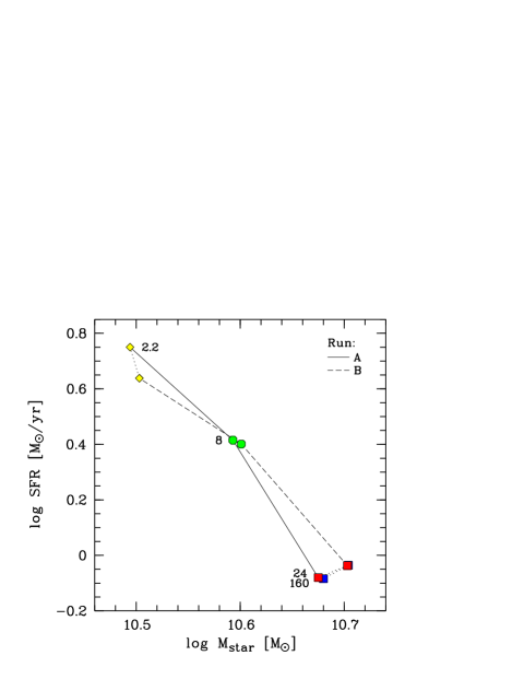
Figure 16: Effect of the reduction of IR filters on the basic galaxy properties total stellar mass and SFR. The diagram provides the sample means and mean errors of these quantities for run A (solid lines) and run B (dashed lines) and different filter combinations. The labels near the symbols indicate the mean wavelength of the last filter in the filter set in $\mu$m. $160$ means that all filters from GALEX $FUV$ to MIPS $160$ $\mu$m are used for the analysis. $2.2$ refers to the $K_{\mathrm{s}}$ band as the reddest filter.

Table 5: Change of the SINGS sample mean for different properties by running CIGALE without IR data

Par.	Run A	Run B
$\log M_{\mathrm{star}}$	$-0.19$	$-0.20$
$\log\mathrm{SFR}$	$+0.83$	$+0.67$
$\log L_{\mathrm{bol}}$	$+0.37$	$+0.31$
$\log L_{\mathrm{dust}}$	$+0.75$	$+0.15$
$\log f_{\mathrm{burst}}$	$+1.05$	$+0.72$
$\log t_{\,\mathrm{D4000}}$	$-0.78$	$-0.71$
$A_{\mathrm{FUV}}$	$+2.16$	$+1.59$
$A_{V}$	$+0.65$	$+0.57$
$\alpha$	$-0.40$	$-0.44$

Since CIGALE allows us to fit photometric data of galaxies ranging from far-UV to far-IR, star-formation-related parameters can be derived in a reliable way due to a full coverage of the dust-affected wavelength range. However, for distant galaxies especially far-IR data are often not available or not sensitive enough. Therefore, we have investigated how results would change if the IR filter set of our sample galaxies was incomplete.

Fig. 16 shows the sample-averaged total stellar mass and SFR for a reduction of the IR filter set. While the full filter set contains 160 $\mu$m as the reddest filter, the most reduced filter set ends at $2.2$ $\mu$m, i.e. the $K_{\mathrm{s}}$ band. There is no significant change of the results as long as the filter set still includes at least one filter (i.e. 24 $\mu$m) which traces the dust emission beyond the PAH regime. Amplitude and slope of the Dale & Helou (DAL02 (2002)) models appear to be well determined in this case. In contrast, the sample means change considerably if the IR is only covered up to 8 $\mu$m, i.e. the region of the PAH emission features, where the Dale & Helou models show little variety only. For run A, $M_{\mathrm{star}}$ decreases by $0.19$ dex and the SFR increases by $0.83$ dex if $K_{\mathrm{s}}$ is the reddest filter. These numbers show that the disregard of mid-IR and far-IR data results in unsatisfying fits for our SINGS test sample. Table 5 shows that many parameters are concerned. Apart from the SFR, important changes are also present for the dust luminosity ($+0.75$ dex), the burst fraction ($+1.05$ dex), and $t_{\,\mathrm{D4000}}$ ($-0.78$ dex). The effective attenuation factors in the far-UV $A_{\mathrm{FUV}}$ and visual $A_{V}$ considerably increase by $2.16$ mag and $0.65$ mag, respectively (cf. Burgarella et al. BUR05 (2005)), if IR data are not considered. Compared to other properties the effect on the mass is relatively small, since this quantity is only indirectly affected by a higher but still minor importance of young stellar populations and the corresponding change of the mass-to-light ratio.

Fig. 16 and Table 5 also illustrate the results for higher uncertainties in the filter fluxes (run B), which indicate lower deviations for most properties. In particular, the changes for $L_{\mathrm{dust}}$ ($+0.15$ dex), $f_{\mathrm{burst}}$ ($+0.72$ dex), and $A_{\mathrm{FUV}}$ ($+1.59$ mag) are significantly reduced. This suggests that the low photometric errors in some filters of run A could force the code into unfavourable fits if no IR data is available. Consistently, the galaxies with SDSS data and consequently lower photometric errors in the optical indicate higher differences in the mean SFR of code runs with and without IR data than objects with corrected optical Dale et al. photometry only.

We have also studied the code results for a filter set without the GALEX $FUV$ and $NUV$ filters. The differences for most parameters are insignificant and the SFR increases by $0.17$ dex (run A) or $0.11$ dex (run B) only. Even $A_{\mathrm{FUV}}$ that directly depends on the UV flux changes by $+0.02$ mag for run A only. An exception is the increase of this quantity by $0.46$ mag for run B. However, this amount is still much lower than the deviations found for the neglection of IR data. Consequently, the UV data of the SINGS galaxies have only little influence on the fit results. This is probably caused by the relatively low weight of these filters in the fitting process (see Table 4). The relatively high uncertainties in the photometry of these two filters do not appear to significantly constrain the star-formation-sensitive UV SEDs of the sample galaxies. Consequently, a lack of IR data can cause striking systematic deviations in the galaxy properties. However, the amount of these deviations probably depends on the SFHs of the galaxies investigated and the filter set available. For example, missing IR data could be better compensated at higher redshifts because of a better filter coverage in the rest-frame UV due to the shift of the observed frame of optical telescopes.

3.3 Results

In the following we present the physical properties of our SINGS sample obtained by means of CIGALE and discuss their reliability (Sect. 3.3.1). We also show relations between the different parameters and compare our results to those from other studies (Sect. 3.3.2).

3.3.1 Expectation values and standard deviations

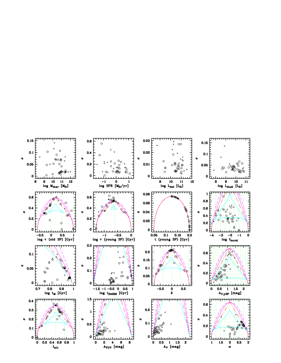
Figure 17: Run A code results for our SINGS test samples with and without SDSS photometry (circles and crosses, respectively). Expectation values and standard deviations are shown for mass-dependent properties ($M_{\mathrm{star}}$, SFR, $L_{\mathrm{bol}}$, and $L_{\mathrm{dust}}$), basic model parameters with at least two selected input values ($\tau_{\mathrm{oSP}}$, $\tau_{\mathrm{ySP}}$, $t_{\,\mathrm{ySP}}$, $f_{\mathrm{burst}}$, $\delta$, $A_{V,\,\mathrm{ySP}}$, $f_{\mathrm{att}}$, and $\alpha$), complex ages ($t_{\,\mathrm{M}}$ and $t_{\,\mathrm{D4000}}$), and effective dust attenuation factors ($A_{\mathrm{FUV}}$ and $A_{V}$). For the basic parameters the selected parameter values are indicated by vertical dotted lines. The different diagnostic curves are described in Fig. 11. All curves depend on the number of parameter values given. For the complex ages and effective attenuation factors we assume 50 which is the number of bins of the parameter probability distributions. The curves for the mass-dependent parameters are not shown, since the errors are much lower than the widths of the object-dependent parameter ranges.

Figure 18: Alternative run B code results for our SINGS test samples. In comparison to Fig. 17, the given errors of the input photometry were increased by 5% added in quadrature in order to account for additional systematic photometric errors and model-inherent uncertainties.

In Fig. 17 (run A) and Fig. 18 (run B) we illustrate the expectation values and standard deviations for the different model parameters of CIGALE for our test sample of 39 SINGS galaxies. We only show results for parameters with PDFs consisting of at least two values. Data points based on photometry with and without SDSS photometry are marked by different symbols (circles and crosses). For evaluating the reliability of the results, the diagrams with mass-independent properties also indicate the diagnostic curves introduced in Sect. 2.3. In fact, the enveloping curves for Gaussian and box-shaped PDFs as well as the “safe” areas for Gaussian distributions are shown.

At first, we discuss the mass-dependent properties $M_{\mathrm{star}}$, SFR, $L_{\mathrm{bol}}$, and $L_{\mathrm{dust}}$ (see Table 2). Typical total stellar masses of about $10^{11}$ M_⊙ and SFRs between $0.1$ and 10 M_⊙yr^-1 reflect that the sample mainly consists of nearby spiral galaxies (see Sect. 3.1). Moreover, the dust luminosities are lower than $10^{11}$ L_⊙, which indicates that luminous IR galaxies (LIRGs) are not present in our sample. The mass-dependent properties are quite well constrained (see Fig. 6 for an example PDF). The typical run A errors range from $0.011$ dex for $L_{\mathrm{bol}}$ to $0.16$ dex for the SFR, which is distinctly smaller than the range of parameter values covered by the sample. This statement is also true for the somewhat higher average errors between $0.013$ and $0.22$ dex for the less constrained run B. The differences between the parameter values for run A and run B are usually within the errors. For the most uncertain mass-dependent property, the SFR, the sample-averaged value increases by $0.05$ dex only if the SFRs of run B instead of run A are considered (see Fig. 16). The mean difference between the SFRs of both runs for individual galaxies is $0.10$ dex.

In contrast to basic model parameters which describe the SFH or the attenuation of the stellar radiation (see Table 1), the mass-dependent global galaxy properties are relatively independent of the details of the models used. Hence, the results for our SINGS test sample can be compared quite comfortably to other studies in this case. The dust luminosity $L_{\mathrm{dust}}$ is relatively easy to measure, since it is directly related to the filter fluxes in the IR (provided that the filters cover the entire relevant wavelength range). Nevertheless, the comparison of $L_{\mathrm{dust}}$ obtained by different studies is a good consistency check. For 13 sample galaxies $L_{\mathrm{dust}}$ determinations are also available by Draine et al. (DRA07b (2007)) who derived them from the SINGS IR SEDs using the Draine & Li (DRA07a (2007)) dust models. The mean difference between our estimates and those of Draine et al. is negligible, since it results in $0.00\pm 0.03$ dex for run A and B. The scatter amounts to $0.1$ dex. A comparison of instantaneous SFRs is more crucial, in particular, if the approaches are completely different. For 29 sample galaxies SFRs of Kennicutt et al. (KEN03 (2003)) are available. They are based on H$\alpha$ emission, which is a thoroughly studied and relatively reliable SFR indicator (see, e.g., Kennicutt KEN98 (1998); Brinchmann et al. BRI04 (2004); Kewley et al. KEW04 (2004); Calzetti et al. CAL07 (2007)). Despite of the completely different methods, our SFRs of run B exhibit a moderate relative scatter of $0.3$ dex and deviate on average by $0.06\pm 0.05$ dex only from those of Kennicutt et al. (see Fig. 19). For run A the SFRs agree even better, since the mean difference amounts to $0.00\pm 0.06$ dex. In any case, this comparison shows that our results for our SINGS test sample are reliable at least for galaxy properties which are relatively independent of the details of the modelling.

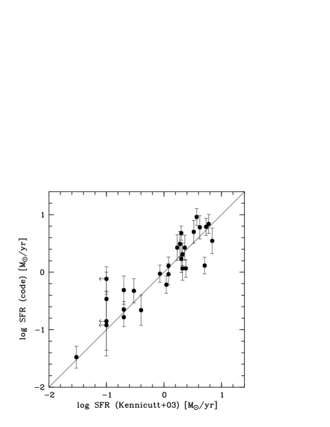
Figure 19: Comparison of the SFRs derived from run B of CIGALE for the SINGS sample and those of Kennicutt et al. (KEN03 (2003)) based on H$\alpha$ emission. Upper limits are indicated by arrows. The error bars of the code results indicate the standard deviation of the SFR probability distribution for each galaxy.

The basic stellar-population-related parameters are the ages and $\tau$ of two Maraston (MARA05 (2005)) models, which are linked by the burst fraction $f_{\mathrm{burst}}$ (see Sect. 2.1.1 and Table 3). We show them in Figs. 17 and 18 excepting the constant $t_{\,\mathrm{oSP}}$. For $\tau_{\mathrm{oSP}}$ and run A the resulting values cover almost the entire investigated range between $0.25$ and $10$ Gyr. However, the errors are relatively high. Most of the data points are close to or on the enveloping curves. In particular, the distribution appears to follow the enveloping curve for box-shaped PDFs. If those distributions were typical (which is difficult to prove because of the small number of parameter values), the $\tau_{\mathrm{oSP}}$ of most galaxies could be classified as “rather low” or “rather high” only. However, the situation appears to be even worse if the results of run B are considered. The lower accuracy of the input photometry causes that for the majority of the objects $\tau_{\mathrm{oSP}}$ is not constrained at all, as the clustering of data points in the peak of the enveloping curves indicates. Consequently, it is safer to assume that the given photometry is not accurate enough to derive $\tau$ values for the old stellar population model. This also appears to be the case for the age and $\tau$ of the young stellar population model. There is only a trend towards relatively high mean $t_{\,\mathrm{ySP}}$ for run A. However, this trend vanishes completely if the results of run B are considered. In contrast, the burst fractions of most sample galaxies are reliable at least in the context of the SFHs allowed by the model grid. Even for run B the data points cluster inside the area of trustworthy results. If run A provided the correct results, the errors in $f_{\mathrm{burst}}$ of part of the galaxies would be even below the grid spacing, which is suggested by a position below the “triangle” in the diagnostic diagram. In any case, small burst fractions below 1% dominate the distribution. No galaxy shows $f_{\mathrm{burst}}>10\%$. This result implies that the current star formation activity tends to be lower than the past average, since the age ratio of the old and young stellar population model is about 80.

The relatively high degree of degeneracy in the SEDs for different SFHs and the enormous amount of possible evolutionary scenarios prevents the reliable derivation of most basic model parameters related to the stellar population. Hence, we also discuss the effective ages $t_{\,\mathrm{M}}$ and $t_{\,\mathrm{D4000}}$ (see Sect. 2.1.1). The mean mass-weighted age $t_{\,\mathrm{M}}$ of 8 Gyr is close to the age of the old stellar population model of 10 Gyr. Consequently, the galaxies under study appear to be dominated by old stars that were formed in the first half of the lifetime of the Universe. However, the exact $t_{\,\mathrm{M}}$ of the individual galaxies is relatively uncertain. While one third of the objects indicates a trustworthy age in the case of run A, there are only a few galaxies with reliable ages in the case of run B. The decrease in errors around 6 Gyr is related to the maximum burst fraction of 10% found in the sample. The age $t_{\,\mathrm{D4000}}$ derived from the strength of the 4000 Å break indicates a wider variety than $t_{\,\mathrm{M}}$ and is quite well constrained even for run B (see also Table 2) and even under consideration of the metallicity dependency of the results (see Sect. 3.2.1). If the mean $t_{\,\mathrm{D4000}}$ of about 1 Gyr is taken, the sample can be divided into a spectroscopically young subsample of 22 galaxies and a mean age of 400 Myr and a complementary old one of 17 galaxies with 3.6 Gyr on average. The relatively wide range in $t_{\,\mathrm{D4000}}$ reflects the variety of galaxy types in SINGS ranging from ellipticals to irregulars (see Kennicutt et al. KEN03 (2003)). While 90% of the young subsample indicates morphological types of Sb and later, only 20% of the old subsample exhibits these types.

Since we do not scale the attenuation law by a $R_{V}$-like constant factor and do not consider the possible presence of 2175 Å absorption features in the SEDs (see Sect. 3.2.1), the shape of the attenuation curve is only determined by the deviation $\delta$ of the slope from a Calzetti law. Figs. 17 and 18 show that $\delta$ of many galaxies is not constrained at all and the rest is highly uncertain. Interestingly, significant deviations of $\delta$ from zero are almost exclusively found for run A and galaxies with SDSS photometry. The latter has not played a role for the parameters discussed so far. This result implies that differences in the shape of the attenuation curve can only be detected if the accuracy of the photometry is in the order of a few percent. For the SINGS sample the accuracy is not good enough for any reliable statements. The situation would probably be better if more and better UV data were available for the SINGS galaxies. However, this is not the case. In comparison to $\delta$ the scaling parameter $A_{V,\,\mathrm{ySP}}$ for the young stellar population, which ranges from $0.15$ to $1.66$ for run A, can be constrained quite well. Most galaxies are in the reliable region of the diagnostic diagram. However, the individual values significantly depend on the run, in particular, if SDSS photometry is available. In this case, the mean $A_{V,\,\mathrm{ySP}}$ changes from $0.67$ for run A to $0.87$ for run B. For the other galaxies the average increase is only half as strong (from $0.89$ to $1.00$). This behaviour can be explained by the stronger run A SED constraints in the optical for galaxies with SDSS photometry and the coupling of $\delta$ and $A_{V,\,\mathrm{ySP}}$ that is suggested by the stability of the dust luminosity. The steeper slopes of the attenuation law for run A ($\langle\delta\rangle=-0.04$ versus $-0.01$ for run B) have to be compensated by lower $A_{V,\,\mathrm{ySP}}$ in order to reach a similar obscuration of the stellar populations by dust. Another attenuation-related parameter is $f_{\mathrm{att}}$ which gives the fraction of $A_{V,\,\mathrm{ySP}}$ for the old stellar population. For individual galaxies the interpretation of the results is uncertain especially for run B. On the other hand, the mean $f_{\mathrm{att}}$ for run A and run B are $0.45\pm 0.03$ and $0.41\pm 0.02$, respectively. This suggests a trend towards $f_{\mathrm{att}}<0.5$ in SINGS. The result is consistent with the fact that many galaxies in our SINGS sample are highly diversified galaxies for which the amount of dust attenuation depends on the age of the stellar population (cf. Fig. 13).

The results for the attenuation at 1500 Å are reliable for most galaxies. The parameter space allowed by the model grid is only partly covered by sample objects. Relatively low $A_{\mathrm{FUV}}$ dominate. The mean values are $1.5$ (run A) and $1.6$ (run B). They correspond to 78% and 69%, respectively, of the values expected for the sample $A_{V,\,\mathrm{ySP}}$ and the Calzetti law ($\delta=0$), which is characterised by $A_{\mathrm{FUV}}/A_{V}=2.55$. Hence, the old $\tau$ model ($t/\tau\sim 10$) significantly contributes even in the far-UV, which is obviously due to the very low burst fractions and low $f_{\mathrm{att}}$ of most sample galaxies. The effective attenuation factors in the visual $A_{V}$ are less reliable than $A_{\mathrm{FUV}}$ and $A_{V,\,\mathrm{ySP}}$. In particular, the run B results are relatively uncertain. This outcome can be explained by the strong dependence of $A_{V}$ on the relatively uncertain attenuation factor $f_{\mathrm{att}}$. The mean $A_{V}$ of both runs is about $0.3$ mag, which corresponds to mean $A_{V}/A_{V,\,\mathrm{ySP}}$ of $0.38$ (run A) and $0.29$ (run B). These values are comparable to the $f_{\mathrm{att}}$ of the sample and suggest that the optical continuum of most sample galaxies is almost completely given by the old $\tau$ model.

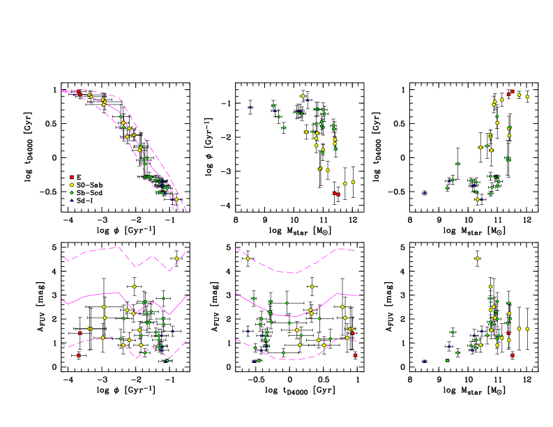
Figure 20: Relations between the total stellar mass $M_{\mathrm{star}}$, the specific SFR $\phi$, the effective age at 4000 Å $t_{\,\mathrm{D4000}}$, and the attenuation in the far-UV $A_{\mathrm{FUV}}$ for the SINGS test sample. The given values and errors are related to run B of CIGALE. The different symbols indicate different morphologies (see legend in upper left subfigure). The solid and dashed curves in the plots not related to $M_{\mathrm{star}}$ show the mean values and $1\,\sigma$ scatter of the model distribution.

Finally, we discuss the shape of the dust emission in the IR. Since we do not consider a hot dust continuum (see Sect. 3.2.1), it is only determined by the $\alpha$ parameter of the Dale & Helou (DAL02 (2002)) templates (see Sect. 2.1.3). Figs. 17 and 18 indicate that low $\alpha$ are very well constrained, while high $\alpha$ are relatively uncertain. This is obviously caused by the degeneracy of the dust emission models for wavelengths shortwards of the emission peak for high $\alpha$. For $\alpha>2.5$ the flux ratio $f_{\nu}(60\,\mu\mathrm{m})/f_{\nu}(100\,\mu\mathrm{m})$ becomes almost constant. Relatively high $\alpha$ dominate the distribution, i.e., the dust temperature tends to be cool. The average sample value of $2.4$ can be compared to the mean $L_{\mathrm{dust}}$ of $6\times 10^{9}$ L_⊙ by using the calibrations of Chapman et al. (CHAP03 (2003)) and Marcillac et al. (MARC06 (2006)) for which we obtain $\alpha\approx 2.1$ and $2.3$. The moderate differences in $\alpha$ could be explained by different properties of the samples used for the calibrations and the SINGS sample. Differences could also be caused by the degeneracy in $f_{\nu}(60\,\mu\mathrm{m})/f_{\nu}(100\,\mu\mathrm{m})$ for high $\alpha$ values and the fact that this flux ratio was taken for the Chapman et al. and Marcillac et al. calibrations instead of $\alpha$.

3.3.2 Correlations

The different galaxy properties derived by CIGALE are not completely independent of each other. For example, the burst fraction $f_{\mathrm{burst}}$ and the two effective ages $t_{\,\mathrm{M}}$ and $t_{\,\mathrm{D4000}}$ are well correlated, since the stellar population properties of the models used mainly depend on the burst fraction (see Sect. 3.3.1). Another example is the relation between the slope modification of the Calzetti law $\delta$ and the attenuation in the visual of the young $\tau$ model $A_{V,\,\mathrm{ySP}}$ based on a relatively stable dust luminosity $L_{\mathrm{dust}}$ discussed in Sect. 3.3.1. Finally, $M_{\mathrm{star}}$, SFR, $L_{\mathrm{bol}}$, and $L_{\mathrm{dust}}$ tend to be correlated because of their dependence on the galaxy mass (see Table 1). Therefore, we restrict our discussion of possible correlations between different galaxy properties on parameters for which the models do not show a direct relation. Moreover, we only consider parameters which were well determined in run B of CIGALE for our SINGS sample (see Table 2) and, therefore, do not suffer from crucial degeneracies. In fact, we discuss the CIGALE output parameters $M_{\mathrm{star}}$, $t_{\,\mathrm{D4000}}$, and $A_{\mathrm{FUV}}$. Moreover, we show the specific SFR $\phi$, i.e. the instantaneous SFR divided by the total mass produced by star formation in the past.

Figure 20 presents the mutual relations of $M_{\mathrm{star}}$, $\phi$, $t_{\,\mathrm{D4000}}$, and $A_{\mathrm{FUV}}$ for our sample of 39 SINGS galaxies. The tightest correlation is found for the quantities $\phi$ and $t_{\,\mathrm{D4000}}$, which depend on stellar population parameters only. It shows that effectively younger stellar populations are linked to higher star formation activity. The correlation obtained is in good qualitative and quantitative agreement with the results of Brinchmann et al. (BRI04 (2004)) for the relation between H$\alpha$-based $\phi$ and D4000 of star-forming SDSS galaxies. However, our distribution is narrower, since a tight correlation is already inherent in the code and the model grid used as the distribution of models in the $\phi$–$t_{\,\mathrm{D4000}}$ plane indicates. For the $M_{\mathrm{star}}$-related diagrams in Fig. 20 correlations based on the selected model grid or the internal structure of the models are not possible, since the mass is the free scaling parameter in the fitting process. Therefore, all mass-related correlations found must have an astrophysical interpretation only. Although the correlation is weaker than those discussed before, the specific SFR clearly tends to decrease with increasing mass, which is in qualitative agreement with previous studies (see, e.g., Brinchmann et al. BRI04 (2004); Salim et al. SALI07 (2007); Buat et al. BUA07 (2007), BUA08 (2008)). Quantitatively, there are some differences due to different sample properties. For example, Salim et al. (SALI07 (2007)) find an average $\phi$ for their sample of star-forming SDSS galaxies at $z\approx 0.1$ that is about $0.4$ dex higher at $10^{10}$ M_⊙ than the value of $-1.3$ dex typical of our sample. The transition from active star formation to a relatively passive evolution is at about $10^{11}$ M_⊙ for our SINGS galaxies. This break in the galaxy properties is even more pronounced for the effective age $t_{\,\mathrm{D4000}}$. The bimodality found is consistent with the results of Kauffmann et al. (2003a , 2003b ) for the SDSS and is reminiscent of the two basic galaxy populations “red sequence” ($\geq 7$ objects) and “blue cloud” ($\geq 19$ objects) discussed in, e.g., Strateva et al. (STR01 (2001)), Baldry et al. (BALD04 (2004)), and Driver et al. (DRI06 (2006)). The galaxies in-between have the highest age uncertainties and could represent at least in part the so-called “green valley”.

In Fig. 20 we also identify the morphological types of our sample galaxies as given in Table 2 (see Kennicutt et al. KEN03 (2003)). For the relations discussed so far, the locus of a galaxy is clearly related to the morphological properties. The earlier the type of a galaxy is, the lower $\phi$ and the higher $t_{\,\mathrm{D4000}}$ and $M_{\mathrm{star}}$ are. These correlations show that our code results are consistent with the well-known dependence of the star formation activity and mass of nearby galaxies on the morphological type (see Roberts & Haynes ROB94 (1994) and Kennicutt KEN98 (1998) for reviews). In this context, the extreme properties of the early-type SBa spiral galaxy NGC 2798 can be understood by the presence of a nuclear starburst that produces a high amount of deeply dust-enshrouded young stars.

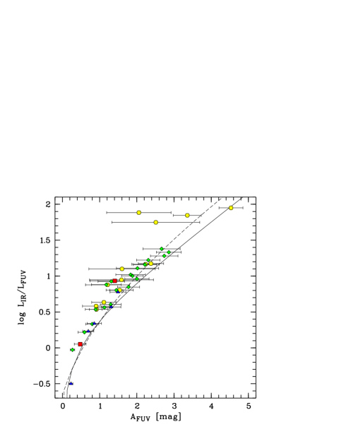
Figure 21: Comparison of the attenuation in the far-UV $A_{\mathrm{FUV}}$ (run B) and the luminosity ratio $L_{\mathrm{IR}}/L_{\mathrm{FUV}}$ as defined by Kong et al. (KON04 (2004)) for our SINGS test sample. For the meaning of the symbols see Fig. 20. Errors can only be shown for the code results. The solid curve exhibits the relation between both parameters for a solar metallicity Maraston (MARA05 (2005)) model with constant SFR and an age of 100 Myr that is reddened by a Calzetti law. The dashed curve shows the corresponding relation for nearby star-forming galaxies of Burgarella et al. (BUR05 (2005)).

No convincing correlation is found for the attenuation at 1500 Å $A_{\mathrm{FUV}}$ and $\phi$ or $t_{\,\mathrm{D4000}}$, i.e. the obscuration of the young stellar population is relatively independent of the star formation activity and history. Concerning the morphology, the latest types (and possibly the ellipticals) in the sample tend to have lower $A_{\mathrm{FUV}}$ than most spiral galaxies. For instance, $A_{\mathrm{FUV}}$ equals $2.00\pm 0.29$ for S0–Sab, $1.64\pm 0.17$ for Sb–Scd, and $0.92\pm 0.22$ for Sd–I. Nevertheless, this trend is much weaker than those found by Buat & Xu (BUA96 (1996)) and Dale et al. (DAL07 (2007)) based on the attenuation tracer $L_{\mathrm{IR}}/L_{\mathrm{FUV}}$ (cf. Fig. 13) instead of $A_{\mathrm{FUV}}$. The latter authors have also found an anticorrelation of $L_{\mathrm{IR}}/L_{\mathrm{FUV}}$ and the specific SFR for intermediate- to late-type galaxies, which cannot be confirmed by us. A possible explanation of these discrepancies could be a systematic weakness of $L_{\mathrm{IR}}/L_{\mathrm{FUV}}$. In contrast to $L_{\mathrm{FUV}}$, $L_{\mathrm{IR}}$ is related to the obscuration of young and old stars. Therefore, significant deviations should appear where dust-absorbed light from cool stars significantly contributes to $L_{\mathrm{IR}}$ (see, e.g., Buat et al. BUA05 (2005); Cortese et al. COR08 (2008) and references therein). The distribution of the sample galaxies in the $A_{\mathrm{FUV}}$–$L_{\mathrm{IR}}/L_{\mathrm{FUV}}$ plane shown in Fig. 21 in comparison to the locus of a typical starburst SED for different opacities indicates that early-type spirals probably exhibit the largest deviations, while the latest types are close to the starburst curve. In detail, the mean deviations of $L_{\mathrm{IR}}/L_{\mathrm{FUV}}$ from the reference curve amount to $0.31\pm 0.07$ for S0–Sab, $0.17\pm 0.02$ for Sb–Scd, and $0.03\pm 0.05$ for Sd–I. As indicated by Fig. 21 early-type spirals also exhibit the largest deviations from the relation between $L_{\mathrm{IR}}/L_{\mathrm{FUV}}$ and $A_{\mathrm{FUV}}$ for nearby star-forming galaxies derived by Burgarella et al. (BUR05 (2005)) (cf. Buat et al. BUA05 (2005); Cortese et al. COR08 (2008)). Consequently, the apparent trend of $L_{\mathrm{IR}}/L_{\mathrm{FUV}}$ with morphology and $\phi$ could be strengthened/produced by the SFH dependence of the luminosity ratio used.

A reliable trend probably exists for the relation between $A_{\mathrm{FUV}}$ and $M_{\mathrm{star}}$. The highest obscurations appear to be present for masses around $10^{11}$ M_⊙, i.e. for galaxies in the transition region. On the other hand, there is also a relatively large scatter in $A_{\mathrm{FUV}}$ of high mass galaxies. For low mass galaxies the dust obscuration tends to decrease with decreasing mass. Late-type galaxies of low mass are obviously characterised by lower dust column densities or a higher porosity of the dust screen in front of young stars compared to galaxies of earlier type (cf. Dale et al. DAL07 (2007)). Apart from irregular and screen-diluting dust distributions, a “lack” of UV-absorbing dust grains could also be due to a deficit of dust production compared to dust destruction or a low metallicity.

4 Discussion and conclusions

We have developed the SED-fitting code CIGALE as a tool for studying basic properties of galaxies in the near and the distant Universe. The models constructed by CIGALE consist of Maraston (MARA05 (2005)) or PEGASE (Fioc & Rocca-Volmerange FIO97 (1997)) stellar population models which are reddened by synthetic attenuation curves based on the Calzetti et al. (CAL00 (2000)) law and which are corrected for spectral lines, and the dust emission templates of Dale & Helou (DAL02 (2002)). The construction of the SFH by two different complex stellar population models with exponentially declining SFRs and different amounts of attenuation enables the code to deal with age-dependent extinction effects (Silva et al. SIL98 (1998); Kong et al. KON04 (2004); Panuzzo et al. PAN07 (2007); Noll et al. NOL07 (2007)), which is crucial to fit “normal” star-forming galaxies that are not characterised by a uniform dust screen in front of the stars (see Fig. 13). The models cover the wavelength range from far-UV to far-IR, which allows the effect of dust on galaxy SEDs to be treated in a consistent way. In the case of dust emission related to a non-thermal source, the balance between the stellar luminosity absorbed by dust and the corresponding emitted luminosity in the IR can be preserved by considering an additional hot dust component.

As our study of the multi-wavelength photometric data of a test sample of 39 nearby galaxies selected from SINGS (Kennicutt et al. KEN03 (2003); Dale et al. DAL07 (2007); Muñoz-Mateos et al. MUN09 (2009)) shows, especially the star-formation-related properties can be derived with high reliability if the photometry reaches from the rest-frame UV to wavelengths greater than 10 $\mu$m (Sect. 3.2.3). Otherwise, the multi-parameter models are not well constrained in the IR and the results can be affected by systematic errors. In the latter case, the models have to be simplified by reasonable a-priori estimates of part of the parameters. Apart from the wavelength coverage of the filter set, the individual uncertainties in filter fluxes also play an important role for the quality of the fit results. Large uncertainties can prevent the derivation of parameters that are nearly degenerated regarding the shape of the galaxy SED such as details of the SFH or the attenuation curve. However, it is more critical if too low photometric errors overconstrain the model parameters, yielding relatively precise but possibly wrong results. Due to unknown systematic errors in the object photometry and the models (see Sect. 3.2.2) it is advisable to assume relative errors between 5% and 10% in minimum. In contrast, the selected approach for the derivation of the expectation values and standard deviations of the different parameters does not significantly affect the code results at least on average (Sect. 3.2.2). The ‘max’ method introduced by us (Sect. 2.2) and the ‘sum’ method (e.g., Kauffmann et al. 2003a ; Salim et al. SALI07 (2007); Walcher et al. WAL08 (2008)) give similar results as long as there are no secondary peaks in the parameter probability distribution which are only poorly populated by models.

The diagnostics of the SED-fitting results of our SINGS test sample has revealed that the most reliable values are obtained for non-basic (by the code derived) model properties such as the total stellar mass $M_{\mathrm{star}}$, the SFR, the effective age $t_{\,\mathrm{D4000}}$, the bolometric luminosity $L_{\mathrm{bol}}$, the dust luminosity $L_{\mathrm{dust}}$, and the far-UV attenuation factor $A_{\mathrm{FUV}}$ (Sect. 3.3.1). Trustworthy results are also found for basic input parameters of the models such as the burst fraction $f_{\mathrm{burst}}$, the $V$-band dust attenuation of the young stellar population $A_{V,\,\mathrm{ySP}}$, and in part the slope of the IR models $\alpha$. However, the latter properties significantly depend on the model grid chosen and are not universal, therefore. The non-basic properties usually show weak model-related constraints only. An example is the upper $t_{\,\mathrm{D4000}}$ limit of 10 Gyr in the sample due to our restrictions regarding the SFHs investigated by the code (Sect. 3.2.1). For the masses given, it has to be taken into account that we provide results for Maraston (MARA05 (2005)) models and Salpeter IMF (see Sect. 2.1.1). In any case, the SFR and $L_{\mathrm{dust}}$ derived indicate good agreement with data from other studies (Sect. 3.3.1).

An investigation of relations between the different reliable galaxy properties has confirmed that the star formation activity of nearby galaxies as traced by the specific SFR $\phi$ and the effective age $t_{\,\mathrm{D4000}}$ depend on morphology (Sect. 3.3.2). Weaker trends are also found for $M_{\mathrm{star}}$ and $A_{\mathrm{FUV}}$. The typical star formation activity significantly changes at $M_{\mathrm{star}}\sim 10^{11}$ M_⊙. This mass range also indicates the most dust-obscured galaxies in our sample. In contrast, far-UV attenuation does not appear to depend on star formation activity. These results show what kind of studies are possible with CIGALE for the data available for the sample of SINGS galaxies investigated. Since the photometric data of the SINGS galaxies is characterised by good coverage of the IR and comparatively modest coverage and quality in the UV, we expect that for other samples especially at higher redshifts the reliability of the different model parameters could be different. For good quality data in the rest-frame UV and optical, we can imagine that stellar population properties and details of the dust attenuation could be better studied than it has been possible for the SINGS sample. On the other hand, the frequently missing information in the far-IR for high-redshift galaxies could significantly affect the quality of $L_{\mathrm{dust}}$ and other star-formation-related parameters. However, instruments such as Herschel or ALMA will improve the situation in future. Hence, we are convinced that CIGALE is a valuable tool for the characterisation of galaxy populations in the near and distant Universe. In a series of forthcoming papers we will demonstrate this by discussing samples of distant galaxies with different selection criteria.

- (1) Baldry, I.K., Glazebrook, K., Brinkmann, J., et al. 2004, ApJ, 600, 681
- (2) Balogh, M.L., Morris, S.L., Yee, H.K.C., et al. 1999, ApJ, 527, 54
- (3) Bolzonella, M., Miralles, J.-M., & Pelló, R. 2000, A&A, 363, 476
- (4) Brinchmann, J., Charlot, S., White, S.D.M., et al. 2004, MNRAS, 351, 1151
- (5) Bruzual, G., & Charlot, S. 2003, MNRAS, 344, 1000
- (6) Buat, V., & Xu, C. 1996, A&A, 306, 61
- (7) Buat, V., Iglesias-Páramo, J., Seibert, M., et al. 2005, ApJ, 619, L51
- (8) Buat, V., Takeuchi, T.T., Iglesias-Páramo, J., et al. 2007, ApJS, 173, 404
- (9) Buat, V., Boissier, S., Burgarella, D., et al. 2008, A&A, 483, 107
- (10) Burgarella, D., Buat, V., & Iglesias-Páramo, J. 2005, MNRAS, 360, 1413
- (11) Calzetti, D., Kinney, A.L., & Storchi-Bergmann, T. 1994, ApJ, 429, 582
- (12) Calzetti, D., Armus, L., Bohlin, R.C., et al. 2000, ApJ, 533, 682
- (13) Calzetti, D., Kennicutt, R.C., Engelbracht, C.W., et al. 2007, ApJ, 666, 870
- (14) Cardelli, J.A., Clayton, G.C., & Mathis, J.S. 1989, ApJ, 345, 245
- (15) Chapman, S.C., Helou, G., Lewis, G.F., & Dale, D.A., et al. 2003, ApJ, 588, 186
- (16) Chary, R., & Elbaz, D. 2001, ApJ, 556, 562
- (17) Cortese, L., Boselli, A., Buat, V., et al. 2006, ApJ, 637, 242
- (18) Cortese, L., Boselli, A., Franzetti, P., et al. 2008, MNRAS, 386, 1157
- (19) da Cunha, E., Charlot, S., & Elbaz, D. 2008, MNRAS, 388, 1595
- (20) Dale, D.A., Helou, G., Contursi, A., Silbermann, N.A., & Kolhatkar, S. 2001, ApJ, 549, 215
- (21) Dale, D.A., & Helou, G. 2002, ApJ, 576, 159
- (22) Dale, D.A., Bendo, G.J., Engelbracht, C.W., et al. 2005, ApJ, 633, 857
- (23) Dale, D.A., Gil de Paz, A., Gordon, K.D., et al. 2007, ApJ, 655, 863
- (24) Dale, D.A., Gil de Paz, A., Gordon, K.D., et al. 2008, ApJ, 672, 735
- (25) Dopita, M.A., Groves, B.A., Fischera, J., & Sutherland, R.S. 2005, ApJ, 619, 755
- (26) Draine, B.T. 2003, ARA&A, 41, 241
- (27) Draine, B.T., & Li, A. 2007, ApJ, 657, 810
- (28) Draine, B.T., Dale, D.A., Bendo, G., et al. 2007, ApJ, 663, 866
- (29) Driver, S.P., Allen, P.D., Graham, A.W., et al. 2006, MNRAS, 368, 414
- (30) Feldmann, R., Carollo, C.M., Porciani, C., et al. 2006, MNRAS, 372, 565
- (31) Fioc, M., & Rocca-Volmerange, B. 1997, A&A, 326, 950
- (32) Fitzpatrick, E.L., & Massa, D. 1990, ApJS, 72, 163
- (33) Fitzpatrick, E.L., & Massa, D. 2007, ApJ, 663, 320
- (34) Gil de Paz, A., Boissier, S., Madore, B.F., et al. 2007, ApJS, 173, 185
- (35) Gordon, K.D., Clayton, G.C., Misselt, K.A., Landolt, A.U., & Wolff, M.J. 2003, ApJ, 594, 279
- (36) Jarrett, T.H., Chester, T., Cutri, R., Schneider, S.E., & Huchra, J.P. 2003, AJ, 125, 525
- (37) Kauffmann, G., Heckman, T.M., White, S.D.M., et al. 2003a, MNRAS, 341, 33
- (38) Kauffmann, G., Heckman, T.M., White, S.D.M., et al. 2003b, MNRAS, 341, 54
- (39) Kennicutt, R.C. Jr. 1998, ARA&A, 36, 189
- (40) Kennicutt, R.C. Jr., Armus, L., Bendo, G., et al. 2003, PASP, 115, 928
- (41) Kewley, L.J., Geller, M.J., & Jansen, R.A. 2004, AJ, 127, 2002
- (42) Kinney, A.L., Calzetti, D., Bohlin, R.C., et al. 1996, ApJ, 467, 38
- (43) Kodama, T., & Arimoto, N. 1997, A&A, 320, 41
- (44) Kong, X., Charlot, S., Brinchmann, J., & Fall, S.M. 2004, MNRAS, 349, 769
- (45) Kroupa, P. 2001, MNRAS, 322, 231
- (46) Krügel, E. 2009, A&A, 493, 385
- (47) Lagache, G., Dole, H., Puget, J.L., et al. 2003, MNRAS, 338, 555
- (48) Lagache, G., Dole, H., Puget, J.L., et al. 2004, ApJS, 154, 112
- (49) Leitherer, C., Li, I.-H., Calzetti, D., & Heckman, T.M. 2002, ApJS, 140, 303
- (50) Madau, P. 1995, ApJ, 441, 18
- (51) Maraston, C. 2005, MNRAS, 362, 799
- (52) Maraston, C., Daddi, E., Renzini, A., et al. 2006, ApJ, 652, 85
- (53) Marcillac, D., Elbaz, D., Chary, R.R., et al. 2006, A&A, 451, 57
- (54) Meiksin, A. 2006, MNRAS, 365, 807
- (55) Meurer, G.R., Heckman, T.M., & Calzetti, D. 1999, ApJ, 521, 64
- (56) Moustakas, J., & Kennicutt, R.C. Jr. 2006, ApJ, 651, 155
- (57) Muñoz-Mateos, J.C., Gil de Paz, A., Zamorano, J., et al. 2009, arXiv:0909.2648
- (58) Noll, S., Mehlert, D., Appenzeller, I., et al. 2004, A&A, 418, 885
- (59) Noll, S., & Pierini, D. 2005, A&A, 444, 137
- (60) Noll, S., Pierini, D., Pannella, M., & Savaglio, S. 2007, A&A, 472, 455
- (61) Noll, S., Pierini, D., Cimatti, A., et al. 2009, A&A, 499, 69
- (62) Panuzzo, P., Granato, G.L., Buat, V., et al. 2007, MNRAS, 375, 640
- (63) Peeters, E., Spoon, H.W.W., & Tielens, A.G.G.M. 2004, ApJ, 613, 986
- (64) Pierini, D., Gordon, K.D., Witt, A.N., & Madsen, G.J. 2004, ApJ, 617, 1022
- (65) Prugniel, P., & Heraudeau, P. 1998, A&AS, 128, 299
- (66) Puget, J.L., & Léger, A. 1989, ARA&A, 27, 161
- (67) Roberts, M.S., & Haynes, M.P. 1994, ARA&A, 32, 115
- (68) Salim, S., Rich, R.M., Charlot, S., et al. 2007, ApJS, 173, 267
- (69) Salimbeni, S., Fontana, A., Giallongo, E., et al. 2009, AIP Conference Proceedings, 1111, 207
- (70) Salpeter, E.E. 1955, ApJ, 121, 161
- (71) Siebenmorgen, R., Krügel, E., & Spoon, H.W.W. 2004a, A&A, 414, 123
- (72) Siebenmorgen, R., Freundling, W., Krügel, E., & Haas, M. 2004b, A&A, 421, 129
- (73) Siebenmorgen, R., & Krügel, E. 2007, A&A, 461, 445
- (74) Silva, L., Granato, G.L., Bressan, A., & Danese, L. 1998, ApJ, 509, 103
- (75) Stecher, T.P. 1969, ApJ, 157, L125
- (76) Stoughton, S., Lupton, R.H., Bernardi, M., et al. 2002, AJ, 123, 485
- (77) Strateva, I., Ivezić, Ž., Knapp, G.R., et al. 2001, AJ, 122, 1861
- (78) Sturm, E., Lutz, D., Tran, D., et al. 2000, A&A, 358, 481
- (79) Walcher, C.J., Lamareille, F., Vergani, D., et al. 2008, A&A, 491, 713
- (80) Witt, A.N., & Gordon, K.D. 2000, ApJ, 528, 799
- (81) Ysard, N., & Verstraete, L. 2009, arXiv:0906.3102