Quantum Phase Transitions of Topological Insulators

Abstract

In this paper, starting from a lattice model of topological insulators, we study the quantum phase transitions among different quantum states, including quantum spin Hall state, quantum anomalous Hall state and normal band insulator state by calculating their topological properties (edge states, quantized spin Hall conductivities and the number of zero mode on a $\pi$-flux). We find that there exist universal features for the topological quantum phase transitions (TQPTs) in different cases : the emergence of nodal fermions at high symmetry points, the non-analytic third derivative of ground state energy and the jumps of the topological ”order parameters”. In particular, the relation between TQPTs and symmetries of the systems are explored : different TQPTs are protected by different (global) symmetries and then described by different topological ”order parameters”.

I Introduction

As the first topologically ordered phase, the Quantum Hall Effect (QHE) is a remarkable achievement in condensed matter physics2 ; qhe . In QHE state, at low temperatures and in strong magnetic fields, quantized Hall conductance can be observed due to the Landau levels formed by states of a two-dimensional electron gas. Just one year later, people discovered the so-called anomalous Hall effect where additional Hall current in the ferromagnetic material was observed3 ; fang . Then, people find that the transverse transport also exists for different spin species, which is called as spin Hall effectzhang1 . Recently, the topological insulators including the quantized spin Hall (QSH) effectkane ; zhang ; berg ; kon and the quantized anomalous Hall (QAH) effecthaldane ; liu become hot issues.

On the one hand, to describe the quantized anomalous Hall state, a class of topological insulators with time-reversal symmetry breaking, the Chern number, so called TKNN integer, is introduced as integrals over the Brillouin zone (BZ) of the Berry field strength thou

$$Q=-\frac{1}{2\pi}\int_{BZ}(\mathbf{\nabla}_{k}\times\mathbf{A})_{z}\,dk_{x}dk_{y}.$$ (1)

Here $A_{j}(k)=-i\langle u_{j}|\nabla_{k}|u_{j}\rangle$ is a Berry connection for single-electron Hamiltonian with the periodic part $u(k)$ of a Bloch state $\psi_{\mathbf{k}}=u(k)e^{i\mathbf{k}\cdot\mathbf{r}}$.

On the other hand, for quantized spin Hall state the spin Chern number $Q_{s}=Q_{\uparrow}-Q_{\downarrow}$ is proposed in Ref.sheng to be the topological invariant to characterize the topological insulators. However, due to spin mixing term (the Rashba term), the spin Chern number $Q_{s}$ is not well defined. Thus for a class of topological insulators with time-reversal symmetry (T-symmetry), due to Kramers degeneracy, Kane and Mele proposed a $Z_{2}$ topological invariantkane ; Roy06 ; Moore06 ; Fu06 ; Essin07

$$(-1)^{\Delta}=\prod_{i=1}^{4}\prod_{m=1}^{N}\xi_{2m}(\vec{k}_{i}),$$ (2)

where $\vec{k}_{i}$ are the four high-symmetry points satisfying $\vec{k}=(0,0)$, $(0,\pi)$, $(\pi,0)$, $(\pi,\pi)$, $\xi_{2m}(\vec{k}_{i})$ is the parity eigenvalue at each of these points, and $N$ is the number of Kramers pairs below Fermi surface. Such $Z_{2}$ topological invariant can be also defined in terms of the spin Chern number

$$\Delta=\frac{1}{2\pi}\int_{EBZ}d^{2}k\,(\mathbf{\nabla}_{k}\times\mathbf{A})_{z}\text{{mod}}2.$$ (3)

Here the integral of the Berry field strength is defined on half of the Brillouin zone. Physically, $\Delta$ is identical with the number of pairs of helical edge modes.

Thus, an interesting issue is the nature of the quantum phase transitions between different types of topological insulators. It is well known that in Landau theory different orders are classified by symmetries. The phase transitions accompanied with (global) symmetry breaking are always described by order parameters. However, Landau’s theory fails to describe the topological quantum phase transition (TQPT). Such type of quantum phase transition cannot be classified by symmetrieswen . Instead, they may be characterized by some topological ”order parameters”, such as the Chern number or $Z_{2}$ topological invariantlifshiz ; volovik ; qi1 .

In this paper, we study the TQPTs between topological insulators and show their physical properties. We find that there are universal features of the TQPTs for different cases : the existence of nodal fermions at high symmetry points, the non-analytic third derivative of ground state energy and the jumps of the topological ”order parameters”. In particular, we find the symmetry protected nature of the TQPTs : different TQPTs are protected by different (global) symmetries and then described by different topological ”order parameters”.

The remainder of the paper is organized as follows. In Sec.II, the two-dimensional lattice models of topological insulators are given. In Sec.III, we focus on the TQPTs between different quantum states with $S^{z}$-conservation (without time reversal symmetry). In this section, the global phase diagram and the critical behavior are obtained. In addition, the topological properties of different quantum states are calculated, including the edge states, the quantized Hall conductivities and the induced quantum numbers on a $\pi$-flux. In Sec.IV, we will study the TQPTs with time reversal symmetry (without $S^{z}$-conservation). In Sec.V, We will study the TQPTs without time reversal symmetry and $S^{z}$-conservation. Finally, the conclusions are given in Sec.VI.

II The lattice models of topological insulators

As a starting point, we consider a lattice Hamiltonian for two-flavor spin-1/2 fermionscom :

$$H_{1}=H_{0}+H_{D},$$ (4)

where

$$H_{0} = \underset{i,\sigma}{\sum}\Psi_{i,\sigma}^{\dagger}\left(\begin{array}[]{cc}-\mu/2&0\\ 0&\mu/2\end{array}\right)\Psi_{i,\sigma}+\underset{i,\sigma}{\sum}\tau_{i,i+x}^{z}\Psi_{i+x,\sigma}^{\dagger}\left(\begin{array}[]{cc}-t&-1/2\\ 1/2&t\end{array}\right)\Psi_{i,\sigma}$$ (12)

$$\underset{i,\sigma}{+\sum}\tau_{i,i+y}^{z}\Psi_{i+y,\sigma}^{\dagger}\left(\begin{array}[]{cc}-t&i\mathrm{sgn}(\sigma)/2\\ i\mathrm{sgn}(\sigma)/2&t\end{array}\right)\Psi_{i,\sigma}+H.c.,$$

$$H_{D} = \underset{i,\sigma}{D\sum}\Psi_{i,\sigma}^{\dagger}\left(\begin{array}[]{cc}-\mathrm{sgn}(\sigma)&0\\ 0&\mathrm{sgn}(\sigma)\end{array}\right)\Psi_{i,\sigma}.$$ (15)

Here $\Psi_{i,\sigma}^{\dagger}=(\psi_{i,A\sigma}^{\dagger},\psi_{i,B\sigma}^{\dagger})$ is a two-component particle operator where $\sigma\equiv\uparrow,\downarrow$ is the spin index, $A$, $B$ denote the flavor indices and $i$ labels the site on the square lattice. $t$ is the real hopping parameters. $\mu$ is the orbital splitting energy. $D$ is an ”effective” magnetic field which was first introduced in Ref.liu phenomenologically which may be induced by local magnetic moments. The bond variables $\tau_{i,j}^{z}$ is set to $+1$ everywhere at the beginning. For the case of $D>0$, we set the $\mathrm{sgn}(\sigma)D$ is positive for spin-up while the $\mathrm{sgn}(\sigma)D$ is negative for spin down. Without $D$ terms, the model in Eq.[3] is really a lattice realization of the Kane-Mele model proposed in Ref.ran ; ran1 , of which the ground state is a topological insulator for $t>1/4$.

Using the Fourier transform $\Psi_{i}=\frac{1}{\sqrt{N}}\underset{k}{\sum}e^{-ik\cdot R_{i}}\Psi_{k},$ we can transform the four field operators on each site into momentum space $\Psi_{k}^{\dagger}=(\Psi_{k,A\uparrow}^{\dagger},\Psi_{k,B\uparrow}^{\dagger},\Psi_{k,A\downarrow}^{\dagger},\Psi_{k,B\downarrow}^{\dagger}).$ Then we get

$$H_{k}=\sum_{k}\Psi_{k}^{\dagger}\left(\begin{array}[]{cc}h_{+(k)}&0\\ 0&h_{-(k)}\end{array}\right)\Psi_{k},$$ (16)

where, for the spin up part

$$h_{+(k)}=\left(\begin{array}[]{cc}-\frac{\mu}{2}-2t(\cos k_{x}+\cos k_{y})-D&\sin k_{y}+i\sin k_{x}\\ \sin k_{y}-i\sin k_{x}&\frac{\mu}{2}+2t(\cos k_{x}+\cos k_{y})+D\end{array}\right).$$

and for the spin down part

$$h_{-(k)}=\left(\begin{array}[]{cc}-\frac{\mu}{2}-2t(\cos k_{x}+\cos k_{y})+D&-(\sin k_{y}-i\sin k_{x})\\ -(\sin k_{y}+i\sin k_{x})&\frac{\mu}{2}+2t(\cos k_{x}+\cos k_{y})-D\end{array}\right).$$

The energy spectrum is then given by diagonalizing the Hamiltonian

$$E_{k}=\pm\sqrt{(\sin^{2}k_{y}+\sin^{2}k_{x})+(\frac{\mu}{2}+2t(\cos k_{x}+\cos k_{y})\pm D)^{2}}.$$ (17)

It is obvious that the term of $\mathrm{sgn}(\sigma)D$ breaks the T-symmetry,

$$H_{1}(k)\neq\Theta^{-1}H_{1}^{T}(-k)\Theta$$ (18)

where $\Theta=i\sigma_{y}K$ ($\sigma_{x,y,z}$ are Pauli matrices and $K$ stands for complex conjugation). However, the model has an additional spin rotation symmetry around $z$-direction as

$$H_{1}=e^{-i\theta\sigma_{z}}H_{1}e^{i\theta\sigma_{z}}.$$ (19)

In addition, by adding the Rashba term to $H_{0}$, we get another lattice model $H_{2}=H_{0}+H_{R}$ where

$$H_{R}=\sum_{i}R(\Psi_{i,\uparrow}^{\dagger}\Psi_{i+x,\downarrow}-\Psi_{i,\downarrow}^{\dagger}\Psi_{i+x,\uparrow})+\sum_{i}iR(\Psi_{i,\uparrow}^{\dagger}\Psi_{i+y,\downarrow}-\Psi_{i\downarrow,}^{\dagger}\Psi_{i+y,\uparrow})+H.c..$$ (20)

By using the Fourier transform we get

$$H_{R}=\sum_{k}\Psi_{k}^{\dagger}\left(\begin{array}[]{cc}0&R(\sin k_{y}+i\sin k_{x})\tau^{0}\\ R(\sin k_{y}-i\sin k_{x})\tau^{0}&0\end{array}\right)\Psi_{k},$$ (21)

where, $\tau^{0}$ is the unit matrix. Now there is T-symmetry

$$H_{2}(k)=\Theta^{-1}H_{2}^{T}(-k)\Theta.$$ (22)

However $S_{z}$ is not a good quantum number due to

$$H_{2}\neq e^{-i\theta\sigma_{z}}H_{2}e^{i\theta\sigma_{z}}.$$ (23)

Furthermore, one may consider a lattice model $H_{3}$ with both $H_{D}$ and $H_{R}$ as $H_{3}=H_{0}+H_{D}+H_{R}$. Now the Hamiltonian $H_{3}$ has neither T-symmetry nor $S_{z}$-conservation due to

$$H_{3}(k)\neq\Theta^{-1}H_{3}^{T}(-k)\Theta$$ (24)

and

$$H_{3}\neq e^{-i\theta\sigma_{z}}H_{2}e^{i\theta\sigma_{z}}.$$ (25)

In the following parts we will study TQPTs by keeping different symmetries based on different lattice models $H_{1,2,3}$.

III TQPTs with $S^{z}$-conservation : $D\neq 0,$ $R=0$

III.1 Global phase diagram

In this section, to learn the TQPT of topological insulators with $S^{z}$-conservation ($D\neq 0,$ $R=0$)$,\$we focus on $H_{1}=H_{0}+H_{D}.$

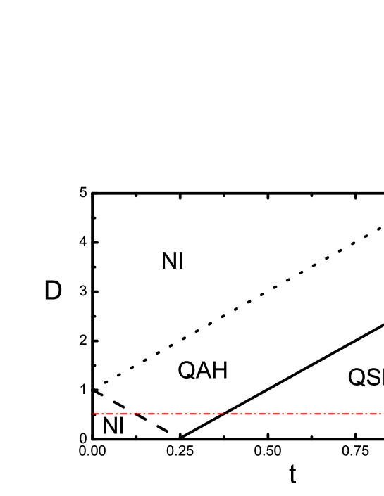
Figure 1: The global quantum phase transition diagram. The solid, dashed and dotted lines are $-\mu/2+4t=D,$ $\mu/2-4t=D,$ $\mu/2+4t=D$ respectively. these lines consist of the boundary of the quantum anomalous Hall state. The solid line is the critical line separating the QAH and QSH. The dashed and dotted lines are the critical lines separating the QAH and NI. The dash dot line intersects the solid and dotted lines at the points $(t,$ $D)=(0.125,$ $0.5)$ and $(t,$ $D)=(0.375,$ $0.5).$ The parameter $\mu$ is set to be 2.

By calculating the phase boundary with zero fermion energy, we obtain the phase boundary,

$$1\pm 4t=\pm D.$$ (26)

In the global phase diagram which was shown in Fig.1, there exist three phases : QAH state, QSH State and NI state. Taking $D=0.5$ as an example (the horizontal dash dot line in Fig.1), one can see that the QSH state occurs in the region of $t>0.375$. Although the T-symmetry is broken in this region, the topological properties of the QSH state is preserved (the edge states, the quantized Hall conductivities and the induced quantum numbers on a $\pi$-flux). With the decrease of $t$, the system turns into a QAH state in the region of $0.375>t>0.125.$ In this region, one may find that the topological properties are different from that in the QSH state. In the region of $0.125>t>0$, the ground state turns into a normal band insulator with trivial topological properties. In Fig.1, the solid, dashed and dotted lines are given by $-1+4t=D,$ $1-4t=D$ and $1+4t=D$ which denote the phase boundaries obtained above.

III.2 Topological ”order parameter” - Spin Chern number

When $D\neq 0,$ one can not use the $Z_{2}$ topological number to classify the topological insulators. However $S_{z}$ is still a good quantum number, the Hamiltonian is decoupled for each spin component, then the spin Chern number is suitable to characterize different quantum states. The Chern number of each spin component is defined as $Q_{\uparrow,\downarrow}.$

Now we write the Hamiltonian of up-spin and down-spin fermions into

$$H=\sum_{k}\Psi_{k\uparrow}^{{\dagger}}\mathbf{N}_{\uparrow}(k)\Psi_{k\uparrow}+\sum_{k}\Psi_{k\downarrow}^{{\dagger}}\mathbf{N}_{\downarrow}(k)\Psi_{k\downarrow,}$$ (27)

where $\Psi_{k\uparrow}=(\Psi_{k,A\uparrow},\Psi_{k,B\uparrow})^{T}$ and $\Psi_{k\downarrow}=(\Psi_{k,A\downarrow},\Psi_{k,B\downarrow})^{T}$. In above Hamiltonian, we have define

$$\mathbf{N}_{\uparrow}(k) = N_{\uparrow,1}^{1}\tau^{x}+N_{\uparrow,2}\tau^{y}+N_{\uparrow,3}\tau^{z},\text{ }$$ (28)

$$\mathbf{N}_{\downarrow}(k) = N_{\downarrow,1}^{1}\tau^{x}+N_{\downarrow,2}\tau^{y}+N_{\downarrow,3}\tau^{z},$$

where

$$N_{\uparrow,3} = -1-2t[\cos k_{x}+\cos k_{y}]-D,$$ (29)

$$N_{\uparrow,2} = -\sin k_{x},\text{ }N_{\uparrow,1}=\sin k_{y},$$

and

$$N_{\downarrow,3} = -1-2t[\cos k_{x}+\cos k_{y}]+D,$$ (30)

$$N_{\downarrow,2} = -\sin k_{x},\text{ }N_{\downarrow,1}=-\sin k_{y}.$$

$\tau^{x,y,z}$ are Pauli matrices.

Now two Chern numbers $Q_{\uparrow}$ and $Q_{\downarrow}$ for up-spin particle and down-spin particle are obtained asqi1 ,

$$Q_{\uparrow}=\frac{1}{8\pi^{2}}\int_{\Omega}d^{2}k[\mathbf{n}_{\uparrow}\cdot\partial_{x}\mathbf{n}_{\uparrow}\times\partial_{y}\mathbf{n}_{\uparrow}],$$ (31)

and

$$Q_{\downarrow}=\frac{1}{8\pi^{2}}\int_{\Omega}d^{2}k[\mathbf{n}_{\downarrow}\cdot\partial_{x}\mathbf{n}_{\downarrow}\times\partial_{y}\mathbf{n}_{\downarrow}].$$ (32)

Here $\mathbf{n}_{\uparrow}$ and $\mathbf{n}_{\downarrow}$ are defined as $\mathbf{n}_{\uparrow}=\frac{\mathbf{N}_{\uparrow}}{|\mathbf{N}_{\uparrow}|}$ and $\mathbf{n}_{\downarrow}=\frac{\mathbf{N}_{\downarrow}}{|\mathbf{N}_{\downarrow}|}$, respectively. $\Omega$ is the area of Brillouin zone.

In the QSH state, for up-spin, the Chern number is $Q_{\uparrow}=1$; for down-spin, it is $Q_{\downarrow}=-1$. So the total Chern number is zero $Q=Q_{\uparrow}+Q_{\downarrow}=0$. However there is nonzero spin Chern number $Q_{s}=Q_{\uparrow}-Q_{\downarrow}=2$. In the QAH state, for up-spin, the Chern number is $Q_{\uparrow}=1$; for down-spin, it is $Q_{\downarrow}=0$. So the total Chern number is obtained as $Q=Q_{\uparrow}+Q_{\downarrow}=1$ and spin Chern number $Q_{s}=Q_{\uparrow}-Q_{\downarrow}=1$. In NI state, the Chern number is zero for each spin component, $Q=Q_{\uparrow}=Q_{\downarrow}=0$. From the results of the Chern number of different quantum states, one may imagine that the QAH state may be considered as half of the QSH state. This statement is also supported by the following calculations of other topological parameters.

In order to give a clear comparison of the total Chern number and the spin Chern number in different quantum states, we list the results in Table.1.

QSH QAH  NI

Total Chern number $0$ $1$ $0$

Spin Chern number $$2 1 0$$

From the Table. 1, one can see obviously that the spin Chern number can be regarded as the topological invariant to characterize the topological insulators and their quantum phase transitions for the Hamiltonian with $S^{z}$-conservationsheng ; pro .

III.2.1 Edge states

In this part, we calculate the edge states in different states.

From the relationship between the spin Chern number and the number of the (chiral) edge states for each spin component $n_{\uparrow,\downarrow},$ we have

$$n_{\uparrow} = \frac{1}{8\pi^{2}}\int_{\Omega}d^{2}k\text{ }\mathbf{n}_{\uparrow}\cdot\partial_{x}\mathbf{n}_{\uparrow}\times\partial_{y}\mathbf{n}_{\uparrow},$$ (33)

$$n_{\downarrow} = \frac{1}{8\pi^{2}}\int_{\Omega}d^{2}k\text{ }\mathbf{n}_{\downarrow}\cdot\partial_{x}\mathbf{n}_{\downarrow}\times\partial_{y}\mathbf{n}_{\downarrow}.$$

Different Chern numbers also characterize different edge states. In the QSH state, the total number of the edge states is obtained as qi1

$$n = n_{\uparrow}+n_{\downarrow}=0,$$ (34)

$$n_{s} = n_{\uparrow}-n_{\downarrow}=2.$$

Thus there are two edge states with opposite chirality. In the QAH state, there is only one edge state $n=n_{\uparrow}+n_{\downarrow}=1.$ The number of edge states in different phases are plotted in Table.2.

QSH QAH  NI

Edge state’s number $$2$$

The numerical results of the edge states in different states are shown in Fig.2.

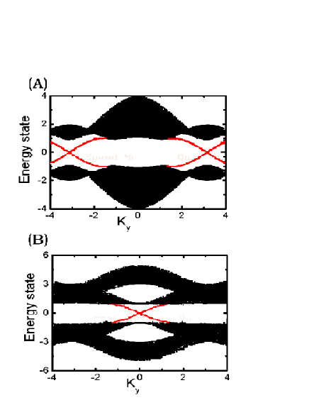
Figure 2: (A): Energy spectrum of the QSH state when the open boundary condition is imposed in x-direction. The parameters are $D=0,$ $t=0.75,$ $\mu=2.$ (B): Energy spectrum of the QAH state when the open boundary condition is imposed in x-direction. The parameters are $D=2,$ $t=0.5,$ $\mu=2.$

From the Table.2, one can see that it is the spin Chern number that determines the number of the edge states in different phases.

III.2.2 Quantized Hall conductivity

Next, we study the quantized Hall conductivity of different states.

We could calculate the charge Hall conductance $\sigma_{xy}$ and the spin-Hall conductance $\sigma_{s,xy}$ for this model in different phases using the standard representationqi1

$$\sigma_{xy}=\sigma_{\uparrow,xy}+\sigma_{\downarrow,xy}.$$ (35)

and

$$\sigma_{s,xy}=\sigma_{\uparrow,xy}-\sigma_{\downarrow,xy.}$$ (36)

where

$$\sigma_{\uparrow,xy} = \frac{e^{2}}{8\pi^{2}h}\int_{\Omega}d^{2}k\text{ }\mathbf{n}_{\uparrow}\cdot\partial_{x}\mathbf{n}_{\uparrow}\times\partial_{y}\mathbf{n}_{\uparrow},$$ (37)

$$\sigma_{\downarrow,xy} = \frac{e^{2}}{8\pi^{2}h}\int_{\Omega}d^{2}k\text{ }\mathbf{n}_{\downarrow}\cdot\partial_{x}\mathbf{n}_{\downarrow}\times\partial_{y}\mathbf{n}_{\downarrow}.$$

Here one can see that the physical consequence of the edge states is just the quantum Hall conductance in our case. In the QSH state, the quantum Hall conductance is obtained as

$$\sigma_{\uparrow,xy}=\frac{e^{2}}{h},\text{ }\sigma_{\downarrow,xy}=-\frac{e^{2}}{h}.$$ (38)

Thus there is no charge Hall conductance, $\sigma_{xy}=\sigma_{\uparrow,xy}+\sigma_{\downarrow,xy}=0$. Instead, the spin-Hall conductance is non-zero, $\sigma_{s,xy}=\sigma_{\uparrow,xy}-\sigma_{\downarrow,xy}=\frac{2e^{2}}{h}.$ In the QAH state, the quantum Hall conductance is obtained as

$$\sigma_{\uparrow,xy}=\frac{e^{2}}{h},\text{ }\sigma_{\downarrow,xy}=0.$$ (39)

Thus both charge Hall conductance and spin-Hall conductance in QAH state are half of the spin-Hall conductance in QSH state

$$\sigma_{xy} = \sigma_{\uparrow,xy}+\sigma_{\downarrow,xy}=\frac{e^{2}}{h},\text{ }$$ (40)

$$\sigma_{s,xy} = \sigma_{\uparrow,xy}-\sigma_{\downarrow,xy}=\frac{e^{2}}{h}.$$

It is pointed out that the spin-Hall conductance is still well defined due to $S_{z}$-conservation in the QAH state.

The spin Hall conductance in different states were shown in Fig.3. The x-axis corresponded to the horizontal dash dot line in Fig.1. We can see that the spin Hall conductance is $0$, $\frac{e^{2}}{h}$ and $\frac{2e^{2}}{h}$ in NI, QAH and QSH respectively. The spin Hall conductance changed from 0 to $\frac{e^{2}}{h}$ at the phase transition point $(t=0.125)$ and changed from $\frac{e^{2}}{h}$ to $\frac{2e^{2}}{h}$ at the phase transition point $(t=0.375)$. In this sense, the TQPTs between QSH, QAH and NI are similar to the quantum Hall plateau transition from Dirac fermion in Ref.lu .

Figure 3: The spin Hall conductance with respected to the three phases: NI, QAH and QSH. The x-axis corresponded to the horizontal dash dot line in Fig.1.

The clearly comparison of charge-Hall conductance and spin-Hall conductance in different states are shown in Table.3

QSH QAH  NI

Charge Hall conductance ($$\frac{e^{2}}{h}$$)

Spin Hall conductance ()

This table indicates that spin Chern number and total Chern number determine charge Hall conductance and the spin-Hall conductance in different states, respectively.

III.2.3 Induced quantum numbers on a $\pi$-flux

In addition, we calculate the induced quantum number on a $\pi$-flux in different quantum states. A $\pi$-flux denotes half a flux quantum $(\frac{1}{2}\Phi_{0},$ $\Phi_{0}=\frac{hc}{e})$ on one plaquette of the square lattice which is shown in Fig.4.

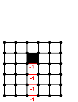
Figure 4: Illustration of a $\pi$-flux in a two-dimensional square lattice ( the gray area ) at the end of a string of minus signs ($-1$) of links.

We calculate the induced quantum number on a $\pi$-flux in the QSH state firstly. In the QSH state, the $\pi$-flux defects defined above may be considered as the Jackiw-Rebbi solitonjackiw . From the numerical results, we find that there are two zero modes of a single $\pi$-flux defect. So such a two dimensional point defect possesses four soliton states, two for each spin (occupied and non-occupied) which are denoted by

$$\mid\uparrow_{+}\rangle\otimes\mid\downarrow_{+}\rangle,\text{ }\mid\uparrow_{-}\rangle\otimes\mid\downarrow_{-}\rangle,$$ (41)

and

$$\mid\uparrow_{-}\rangle\otimes\mid\downarrow_{+}\rangle\text{ }\mid\uparrow_{+}\rangle\otimes\mid\downarrow_{-}\rangle.$$ (42)

Here $\mid\uparrow_{-}\rangle$ and $\mid\downarrow_{-}\rangle$ are the empty states of the zero modes $\Psi_{\uparrow}^{0}(r)$ and $\Psi_{\downarrow}^{0}(r).$ Around a $\pi$ flux, the fermionic operators are expanded as

$$\hat{\Psi}_{\alpha}(r,t) = \sum_{k\neq 0}\hat{b}_{\alpha k}e^{-iE_{k}t}\Psi_{\alpha k}(r)$$

$$+\sum_{k\neq 0}\hat{d}_{\alpha k}^{\dagger}e^{iE_{k}t}\Psi_{\alpha k}^{\dagger}(r)+\hat{a}_{\alpha}^{0}\Psi_{\alpha}^{0}(r),\text{ }$$

where $\hat{b}_{\alpha k}$ and $\hat{d}_{\alpha k}^{\dagger}$ are operators of $k\neq 0$ modes that are irrelevant to the soliton states discussed below. $\hat{a}_{\alpha}^{0}$ are annihilation operators of zero modes and $\alpha$ is the spin index. Thus we have the relationships as

$$\hat{a}_{\uparrow}^{0} \mid \uparrow_{+}\rangle=\mid\uparrow_{-}\rangle,\text{ }\hat{a}_{\uparrow}^{0}\mid\uparrow_{-}\rangle=0,\text{ }$$ (44)

$$\hat{a}_{\downarrow}^{0} \mid \downarrow_{+}\rangle=\mid\downarrow_{-}\rangle,\text{ }\hat{a}_{\downarrow}^{0}\mid\downarrow_{-}\rangle=0.\text{ }$$

We define the induced fermion number operators of the soliton states, $\hat{N}_{\alpha,F}$ with

$$\hat{N}_{\alpha,F}\equiv(\hat{a}_{\alpha}^{0})^{\dagger}\hat{a}_{\alpha}^{0}+\sum\limits_{k\neq 0}(\hat{b}_{\alpha k}^{\dagger}\hat{b}_{\alpha k}-\hat{d}_{\alpha k}^{\dagger}\hat{d}_{\alpha k})-\frac{1}{2},$$

From the relation in Eq.(44), we find that $\mid\uparrow_{\pm}\rangle$ or $\mid\downarrow_{\pm}\rangle$ have eigenvalues of $\pm\frac{1}{2}$ of the induced fermion number operators,

$$\hat{N}_{\uparrow,F}| \uparrow {}_{\pm}\rangle=\pm{\frac{1}{2}}|\uparrow_{\pm}\rangle,\text{ }\hat{N}_{\uparrow,F}|\downarrow_{\pm}\rangle=0,\text{ }$$ (45)

$$\hat{N}_{\downarrow,F}| \downarrow {}_{\pm}\rangle=\pm{\frac{1}{2}}|\downarrow_{\pm}\rangle,\text{ }\hat{N}_{\downarrow,F}|\uparrow_{\pm}\rangle=0.\text{ }$$

From $\hat{N}_{\alpha,F},$ we can define two induced quantum number operators, the total induced fermion number operator $\hat{N}_{F}=\hat{N}_{\uparrow,F}+\hat{N}_{\downarrow,F}$ and the induced quantum spin operator, $\hat{S}^{z}=\frac{1}{2}(\hat{N}_{\uparrow,F}-\hat{N}_{\downarrow,F}).$

Then we calculate two induced quantum numbers defined above. For an insulator state, the ground states are the two degenerate soliton states denoted by $\mid\uparrow_{-}\rangle\otimes\mid\downarrow_{+}\rangle$ and $\mid\uparrow_{+}\rangle\otimes\mid\downarrow_{-}\rangle$. One can easily check that the total induced fermion number on the solitons is zero from the cancelation effect between different spin components

$$\hat{N}_{F}\mid\uparrow_{-}\rangle\otimes\mid\downarrow_{+}\rangle=\hat{N}_{F}\mid\uparrow_{+}\rangle\otimes\mid\downarrow_{-}\rangle=0.$$ (46)

On the other hand, there exists a spin-$\frac{1}{2}$ moment on the soliton states $\mid\uparrow_{-}\rangle\otimes\mid\downarrow_{+}\rangle$ and $\mid\uparrow_{+}\rangle\otimes\mid\downarrow_{-}\rangle,$

$$\hat{S}^{z} \mid \uparrow_{-}\rangle\otimes\mid\downarrow_{+}\rangle=\frac{1}{2}\mid\uparrow_{-}\rangle\otimes\mid\downarrow_{+}\rangle,$$ (47)

$$\hat{S}^{z} \mid \uparrow_{+}\rangle\otimes\mid\downarrow_{-}\rangle=-\frac{1}{2}\mid\uparrow_{+}\rangle\otimes\mid\downarrow_{-}\rangle.$$

The induced spin moment may be straightforwardly obtained by combining the definition of $\hat{S}^{z}$ and Eq. (45) together.

The four different ways of occupation these two zero modes give rise to four different type of fluxons with the following quantum numbers: ($charge=0,$ $spin=\pm\frac{1}{2}$) and ($charge=\pm 1,$ $spin=0$). The results is consistent to that there exist spin-charge separated solitons in the presence of $\pi$-flux with induced quantum numbersqi ; ran ; kou1 .

The charge density of a fluxon in the QSH state on a $24\times 24$ lattice $\Psi_{\uparrow}^{0}(r)\Psi_{\uparrow}^{0}(r)+\Psi_{\downarrow}^{0}(r)\Psi_{\downarrow}^{0}(r)$ is shown in Fig.5. The zero mode is localized around the defect center within a length-scale $\sim m^{-1}.$ Here $m$ is the mass gap of the fermions.

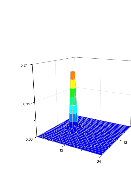
Figure 5: The charge density of a fluxon in the QSH state on a $24\times 24$ lattice with periodic boundary condition. The charge bound to the defect is $\pm e.$

Secondly, we study the zero modes and the induced quantum numbers on a $\pi$-flux in the QAH state. In the QAH state, there is only one zero mode of a single $\pi$-flux defect. The charge densities $\Psi_{\uparrow}^{0}(r)\Psi_{\uparrow}^{0}(r)+\Psi_{\downarrow}^{0}(r)\Psi_{\downarrow}^{0}(r)$ of a pair of defects in the QAH state on a $24\times 24$ lattice with periodic boundary condition was shown in Fig.6. For the two defects, the two zero modes slightly split due to tunneling effect between them.

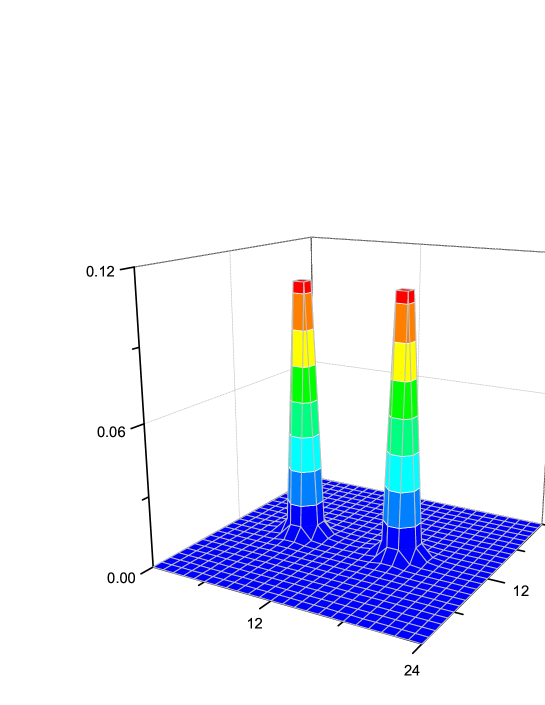
Figure 6: The charge densities of a pair of defects in the QAH state on a $24\times 24$ lattice with periodic boundary condition. The charge bound to the defect is $\pm\frac{e}{2}.$

Thus there are two soliton states, two for up spin particles (occupied and non-occupied) which are denoted by $\mid\uparrow_{+}\rangle$ and $\mid\uparrow_{-}\rangle.$ In contrast, there is no zero mode and soliton states of the $\pi$-flux defect for down spin particles. Similarly we can obtain the eigenvalues of the total induced fermion number operator $\hat{N}_{F}$,

$$\hat{N}_{F}|\uparrow_{\pm}\rangle=\hat{N}_{\uparrow,F}|\uparrow_{\pm}\rangle=\pm{\frac{1}{2}}|\uparrow_{\pm}\rangle.$$ (48)

And the induced quantum spin number on the soliton states $\mid\uparrow_{\pm}\rangle$ is obtained as

$$\hat{S}^{z} \mid \uparrow_{\pm}\rangle=\frac{1}{2}(\hat{N}_{\uparrow,F}-\hat{N}_{\downarrow,F})|\uparrow_{\pm}\rangle$$ (49)

$$= \frac{1}{2}\hat{N}_{\uparrow,F}|\uparrow_{\pm}\rangle=\pm\frac{1}{4}\mid\uparrow_{\pm}\rangle.$$

The occupation (or unoccupation) of this zero mode lead to $N_{F}=\pm\frac{e}{2}$ charge and $S^{z}=\frac{1}{4}$ bound to the defectfranz . Due to $S^{z}$-conservation for the QAH state, the induced quantum spin number $S^{z}=\frac{1}{4}$ is also well defined.

Thirdly, in the NI state, there is no zero mode on a single $\pi$-flux defect. As a result, all induced quantum numbers are zero.

Therefore, in this part we find that the zero mode’s on a $\pi$-flux may also be used to distinguish different quantum phases. These induced quantum numbers are shown in Table.4.

QSH QAH  NI

Zero mode’s number $$2$$

Finally we give a summary. When $D\neq 0,$ because $S_{z}$ is a good quantum number, we can use the spin Chern number $Q_{s}$ to characterize different quantum states as shown in the Table.5.

QSH QAH  NI

Spin Chern number $$Q_{s}$$

Edge state’s number

Zero mode’s number

For the TQPTs from one quantum state to another, the spin Chern number $Q_{s}$ will jump.

III.3 Universal critical behavior of TQPTs

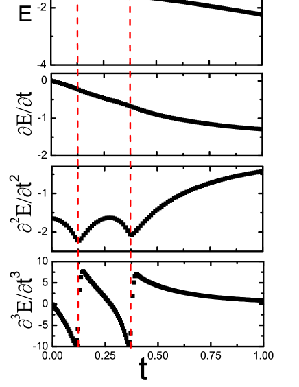
Figure 7: The ground-state energy and its first, second and third derivatives with respect to $t$, where $D=0.5$ (which corresponds to the horizontal dash dot line in Fig.1). It is clear that $E,\frac{\partial E}{\partial t}$ and $\frac{\partial^{2}E}{\partial t^{2}}$ are continuous functions, but $\frac{\partial^{3}E}{\partial t3}$ is discontinuous at the transition points $t=0.125$ and $0.375.$

Another feature of the TQPTs is the non-analyticity of the ground-state energy. The ground-state energy is defined as

$$E=-\sum_{k}(\varepsilon_{+(k)}+\varepsilon_{-(k)})=-\frac{S}{4\pi^{2}}\underset{BZ}{\int}(\varepsilon_{+(k)}+\varepsilon_{-(k)})d^{2}k,$$ (50)

where, $BZ$ denotes the first Brillouin zone and

$$\varepsilon_{\pm(k)}=\sqrt{\sin^{2}k_{y}+\sin^{2}k_{x}+(\frac{\mu}{2}+2t(\cos k_{x}+\cos k_{y})\pm D)^{2}}.$$ (51)

Here $S$ is the area of the system. As an example, we show the TQPT of the model along the line with fixing $D=0.5$ in Fig.1. As illustrated in Fig.7, the ground state energy and its first and second derivatives are continuous for arbitrary $t$, while its third derivative is non-analytic at points $t=0.125$ and $t=0.375$, corresponding to phase transitions NI – QAH and QAH – QSH. It means that the TQPTs are third order. Similar third order TQPTs have been pointed out in other systems where the nodal fermion appearscai .

Let us explain why TQPTs are always third order. The energy dispersions near the quantum phase transitions are shown in Fig.8 and Fig.9. On the line with fixing $D=0.5,$ one can see that there is one nodal point with zero energy in the Brillouin zone, $(\pi,$ $\pi),$ at the quantum phase transition between QSH state and QAH state. Thus the TQPT is dominated by nodal Dirac fermionic excitations at $(\pi,$ $\pi)$. For the TQPT between QAH state and NI state on the line with fixing $D=0.5$, the nodal fermion is also pinned at the point $(\pi,$ $\pi)$.

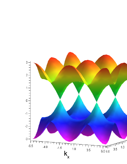
Figure 8: The energy dispersion near the point of phase transition between QSH and QAH. ($k_{x},$ $k_{y}:(-2\pi,$ $2\pi)$)

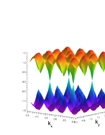
Figure 9: The energy dispersion near the point of phase transition between NI and QAH. ($k_{x},$ $k_{y}:(-2\pi,$ $2\pi)$)

Furthermore, near the critical points of the TQPTs, we get the low energy effective Hamiltonian near the point $(\pi,$ $\pi),$

$$H_{1,\uparrow}\rightarrow m_{\uparrow}\tau^{z}+k_{y}\tau^{x}+k_{x}\tau^{y}$$ (52)

and

$$H_{1,\downarrow}\rightarrow m_{\downarrow}\tau^{z}+k_{y}\tau^{x}-k_{x}\tau^{y}$$ (53)

where $m_{\uparrow}=-1+4t-D$ and $m_{\downarrow}=-1+4t+D$ are the masses of the electrons with up-spin and down-spin, respectively. One can see that crossing the critical point $D=0.5$, $t=0.125$, the mass of the electrons with down-spin changes sign, $\frac{m_{\downarrow}}{\left|m_{\downarrow}\right|}\rightarrow-\frac{m_{\downarrow}}{\left|m_{\downarrow}\right|}.$ Consequently, the Chern number of the electrons with down-spin $Q_{\downarrow}$ changes from $0$ to $1$ that corresponds to the TQPTs from NI state ($Q_{\uparrow}=Q_{\downarrow}=0$) to QAH state ($Q_{\uparrow}=0,$ $Q_{\downarrow}=1$). Similarly, crossing the critical point $D=0.5$, $t=0.375$, the mass of the electrons with up-spin changes sign, $\frac{m_{\uparrow}}{\left|m_{\uparrow}\right|}\rightarrow-\frac{m_{\uparrow}}{\left|m_{\uparrow}\right|}$, that leads to the Chern number of the electrons with up-spin $Q_{\uparrow}$ changes from $0$ to $1$, corresponding to the TQPTs from QAH state ($Q_{\uparrow}=0,$ $Q_{\downarrow}=1$) to QSH state ($Q_{\uparrow}=1,$ $Q_{\downarrow}=1$). For a special TQPT at ($D=0$), the mass of the electrons with up-spin $m_{\uparrow}=-1+4t$ is equal to the mass of electrons with down-spin $m_{\downarrow}=-1+4t.$ The changes of mass sign will lead to the jumps of spin Chern number, $\Delta Q_{\uparrow}=\Delta Q_{\downarrow}=1,$ that corresponds to a direct topological quantum phase transition from NI state ($Q_{\uparrow}=Q_{\downarrow}=0$) to QSH state ($Q_{\uparrow}=1,$ $Q_{\downarrow}=1$)shu . Fig.10 is a scheme to illustrate the relationship between the jump of the spin Chern number and the change of mass sign.

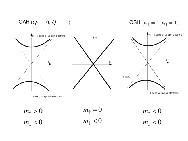
Figure 10: Illustration of the relationship between the jump of the spin Chern number and the change of mass sign.

On the other hand, due to the existence of the nodal fermion, the TQPTs with mass sign changes ($m_{\uparrow,\downarrow}\rightarrow-m_{\uparrow,\downarrow}$) are always third order. One may use the low energy approximation, $E(k)=\sqrt{k^{2}+m_{\uparrow,\downarrow}^{2}},$ and then get the ground state energy as

$$E(m_{\uparrow,\downarrow})\sim-|m_{\uparrow,\downarrow}|^{3}+\mathrm{const}_{\uparrow,\downarrow}$$ (54)

where $\mathrm{const}_{\uparrow,\downarrow}$ is a constantcai . It is obvious that the third order derivative of $E(m_{\uparrow,\downarrow})$ to $m_{\uparrow,\downarrow}$ is discontinuous at the point $m_{\uparrow,\downarrow}=0$.

In brief, for the TQPTs, NI – QAH and QAH – QSH, the changes of the mass sign $m_{\uparrow,\downarrow}\rightarrow-m_{\uparrow,\downarrow}$ reflect the jumps of the (spin) Chern numbers ($\Delta Q_{s}\neq 0$). As a result, third order phase transitions is a universal feature of the TQPTs.

III.4 Finite temperature properties

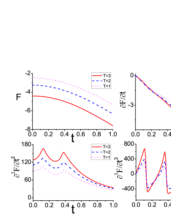
Figure 11: The free energy and its first, second and third derivatives with respect to $t$, where $D=0.5$ (which corresponds to the horizontal dash dot line in Fig.1). It is clear that $F,$ $\frac{\partial F}{\partial t}$, $\frac{\partial^{2}F}{\partial t^{2}}$ and $\frac{\partial^{3}F}{\partial t3}$ are all analytic.

At finite temperature ($T\neq 0$), the free energy $F$ is defined by

$$F=-T\int\frac{d^{2}k}{(2\pi)^{2}}2\ln(\cosh(\varepsilon_{+(k)}+\varepsilon_{-(k)})).$$ (55)

Here we set $k_{B}=1$. We calculate the derivatives of the free energy which are shown in Fig.11. One can see that the free energy and its first, second, third derivatives are all analytic without singularity at $T\neq 0$. The results means that at finite temperature, there is no real phase transition, instead one gets crossovers. This result is consistent with that of the TQPT between QAH state and NI state in Ref.cai .

III.5 Stability of the TQPTs

Finally we discuss the stability of the TQPTs. At the critical points, there always exist nodal fermion with zero energy at $(\pi,$ $\pi)$. Thus at the critical points, we linearize the dispersion at $(\pi,$ $\pi)$ and get a low energy effective Dirac Hamiltonian of nodal fermions,

$$H_{1} = \sum_{k}\Psi_{k,\uparrow}^{\dagger}(\tau^{x}k_{y}+\tau^{y}k_{x})\Psi_{k,\uparrow}+\sum_{k}\Psi_{k,\downarrow}^{\dagger}(\tau^{y}k_{x}-\tau^{x}k_{y})\Psi_{k,\downarrow}$$

$$= \sum_{k}\Psi_{k}^{\dagger}\sigma_{z}\gamma_{i}k_{i}\Psi_{k},$$

where the $\gamma$ matrices are defined by $\gamma_{x}=\tau^{2}$ and $\gamma_{y}=\tau^{1}$.

Then we consider effect of short range interactions. For example, one may add an on-site four-fermi interaction $H_{int}=U(\Psi^{\dagger}\Psi)^{2}$ to $H_{1}.$ Now we get an effective three dimensional Gross-Neveu model with the Lagrangiangross

$$L_{GN}=i\Psi^{\dagger}\gamma_{\mu}\partial_{\mu}\Psi+U(\Psi^{\dagger}\Psi)^{2}.$$ (57)

It is known in large-N limit, the Callan-Symanzik function of $\beta(U)$ is $\beta(U)=-\frac{\lambda U}{2\pi}+U$. For a small interaction, $U\rightarrow 0,$ the four-fermi interaction is irrelevant. That means the TQPTs is stable against the small on-site four-fermi interaction. Similarly, considering other types of short range interaction with $S_{z}$-conservation, one may get the same results: they are irrelevant and the nodal fermions are stable.

IV TQPTs with T-symmetry : $D=0,$ $R\neq 0$

IV.1 Global phase diagram

In this section, to learn the TQPT of topological insulators with T-symmetry, $D=0,$ $R\neq 0,\$we focus on $H_{2}=H_{0}+H_{R}$ and show the effect of the Rashba term.

Figure 12: The global phase diagram at $D=0$.

From the global phase diagram in Fig.12, one can see that there exist three quantum phases : QSH state, NI state and gapless semi-metal. The solid line divides the gapped phases and the gapless semi-metal. As shown in Fig.13, when one fixes $t$ at $0.375$, the energy gap will decrease with the increase of $R$ and close at $R=1.$ However, the phase boundary (the dashed line in Fig.12) between the QSH state and NI state doesn’t change by the Rashba term.

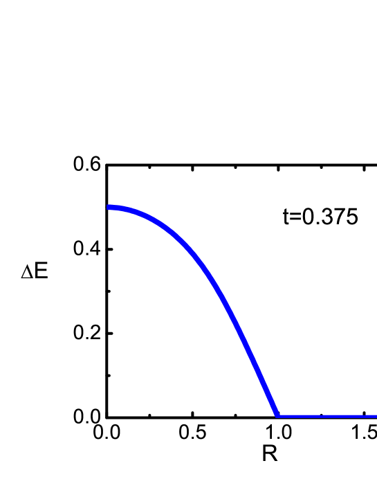
Figure 13: The energy gap with respect to the Rashba term $R$ at $t=0.375$.

IV.2 Topological ”order parameter” - $Z_{2}$ topological invariant

To see the topological properties of the Hamiltonian with T-symmetry but without $S_{z}$-conservation, we calculate the edge states and the zero mode’s number on a $\pi$-flux in different quantum states. In the QSH state, from the numerical results, we find that there also exist two zero modes of a single $\pi$-flux defect. The charge density of a fluxon in the QSH state on a $24\times 24$ lattice is shown in Fig.14. In the NI state, there is no such zero mode on a single $\pi$-flux defect. On the other hand, the results of the edge states are shown in Fig.15, from which we find that there are two edge states in QSH state, while in the NI state, there is no edge state.

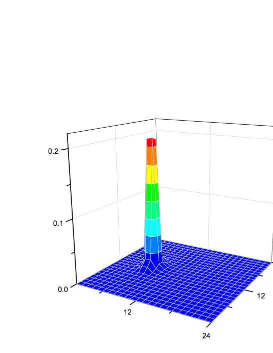
Figure 14: The charge density of a fluxon in the QSH phase on a $24\times 24$ lattice with periodic boundary condition. The charge bound to the defect is $\pm e.$

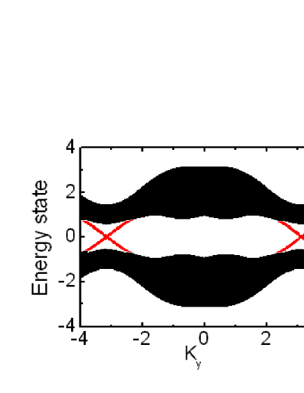
Figure 15: Energy spectrum of the QSH state when the open boundary condition is imposed in x-direction. The parameters are $R=0.4,$ $t=0.5,$ $\mu=2.$

Above results indicate that the T-symmetry indeed protects the topological properties of the QSH state. Thus we calculate the $Z_{2}$ topological invariant $(-1)^{\Delta}=\prod_{i=1}^{4}\prod_{m=1}^{N}\xi_{2m}(\vec{k}_{i})$ in different gapped quantum state. For the four high-symmetry points, $(0,0)$, $(0,\pi)$, $(\pi,0)$, $(\pi,\pi)$, the eigenvalues below Fermi surface $E_{F}$ of this system are

$$1+4t,\text{ }1,\text{ }1,\text{ }1-4t,$$ (58)

respectively. TQPT occurs at $t=1/4$. For $t<1/4,$ the four eigenvalues are all positive. Using the formula mentioned above, one can see that the $Z_{2}$ topological invariant $(-1)^{\Delta}$ is $1$ which means the system is in the NI phase. For $t>1/4$, one eigenvalue is negative while the others are all positive. It is obvious that the $Z_{2}$ topological invariant $(-1)^{\Delta}$ is $-1$ which means the system is in the QSH phase.

Table.6 shows the relationship between the $Z_{2}$ topological invariant $(-1)^{\Delta}$ and the topological properties of the quantum states,

$$D=0,$$ QSH  NI

topological invariant

Edge state’s number

Zero mode’s number on a -flux

IV.3 Universal critical behavior of TQPT

To study the universal critical behavior of the TQPT between QSH state and NI state without $S_{z}$-conservation, we calculate the derivatives of the ground-state energy $E$. Here the ground-state energy becomes $E=-\sum_{k}(\varepsilon_{+(k)}+\varepsilon_{-(k)})$ where

$$\varepsilon_{\pm(k)}=\sqrt{\sin^{2}k_{y}+(R\sqrt{(\sin^{2}k_{x}+\sin^{2}k_{y})}\pm\sqrt{\sin^{2}k_{y}+(\frac{\mu}{2}+2t(\cos k_{x}+\cos k_{y}))^{2}})^{2}}.$$ (59)

We show the TQPT along the line with fixing $R=0.2$. As illustrated in Fig.16, the third derivative is non-analytic at points $t=0.25$, corresponding to quantum phase transitions NI – QSH. So the TQPT is also third order.

Figure 16: The ground-state energy and its first, second and third derivatives with respect to $t$, It is clear that $E,\frac{\partial E}{\partial t}$ and $\frac{\partial^{2}E}{\partial t^{2}}$ are continuous functions, but $\frac{\partial^{3}E}{\partial t3}$ is discontinuous at the transition point $t=0.25$.

The energy dispersion near the quantum phase transition is shown in Fig.17. From the dispersion of the electrons near the critical points, we find that the TQPT is also dominated by the nodal fermion near the point $(\pi,$ $\pi).$

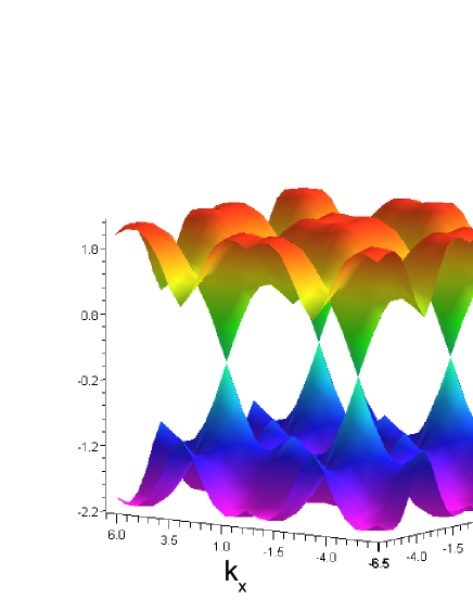
Figure 17: The energy dispersion near the quantum phase transition. The parameters are $t=0.25$ and $R=0.2.$

Let us explain why the TQPT between QSH state and NI state are also third order. When $R\neq 0,$ there is no $S_{z}$-conservation and one cannot define the spin Chern number. So we cannot use the jump of the Chern number to understand the TQPT. However, from the definition of the $Z_{2}$ topological invariant, we find that near the TQPT, the mass signs of the two kinds of low energy fermions ($m=-1+4t$) are determined by the $Z_{2}$ topological invariant $(-1)^{\Delta}$ (See Eq.58). Consequently, for the TQPT between NI state ($(-1)^{\Delta}=1$) to QSH state ($(-1)^{\Delta}=-1$), the sudden change of the $Z_{2}$ topological invariant will lead to the change of mass sign of low energy fermions.

In brief, for the TQPT, NI – QSH, the change of mass sign come from the sudden change of the $Z_{2}$ topological invariant. As a result, the TQPT between NI state and QSH state is always third order.

V TQPTs without T-symmetry and $S_{z}$-conservation : $D\neq 0,$ $R\neq 0$

In this section, we study the TQPTs of topological insulators without T-symmetry and $S_{z}$-conservation, $D\neq 0,$ $R\neq 0\$based on $H_{3}=H_{0}+H_{D}+H_{R}.$

Figure 18: The global phase diagram at $D=0.5.$

We take $D=0.5$ as an example (which corresponds to the horizontal dash dot line in Fig.1). The results are illustrated in Fig.18. One can see that in the phase diagram there exist three phases : two NI states and one QAH state. The QAH state is robust while arbitrary small $R$ will destroy the QSH state. To understand the disappearance of the QSH state, on the one hand the evolution of the energy levels of zero modes on a $\pi$-flux with $R$ at the point $D=0.5,$ $t=0.75$ is plotted in Fig.19. The black bars denote the continuum spectrum while the black triangles denote the energy levels of zero modes on a $\pi$-flux. One can see that the degeneracy of zero modes is lifted by the Rashba term. With increasing $R,$ the energy gap of the continuum spectrum decreases, while the energy splitting of the zero modes $\Delta E$ increases. On the other hand, the evolution of edge states in QSH state with the Rashba term is shown in Fig.20. When $R\neq 0$ and $D\neq 0,$ due to the hybridization of two edge states, the edge states in the QSH state open an energy gap. In contrast, in the QAH phase, the edge state and the zero modes are all stable.

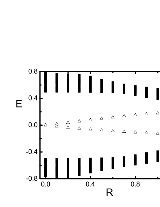
Figure 19: The evolution of the energy spectrum of the system with a $\pi$-flux at $D=0.5,$ $t=0.75$.

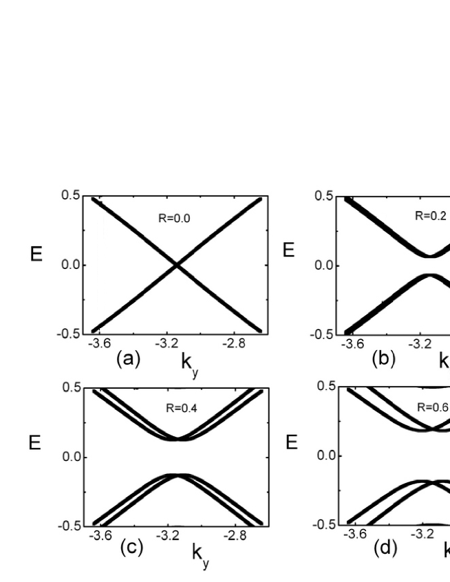
Figure 20: The evolution of edge states in QSH state with the Rashba term $R$ at $D=0.5,$ $t=0.75$. a, b, c and d correspond to $R=0$, $R=0.2$, $R=0.4$ and $R=0.6$ respectively.

In this case (a system without T-symmetry and $S_{z}$-conservation), the TKNN integer $Q$ can be regarded as an ”order parameter” to characterize different quantum states, $Q=-\frac{1}{2\pi}\int_{BZ}(\mathbf{\nabla}_{k}\times\mathbf{A})_{z}\,dk_{x}dk_{y}.$ Table.7 shows the relationship between the TKNN integer $Q$ and the topological properties of the quantum states,

TKNN integer Q10Edge state’s number10Zero mode’s number on π-flux10.fragments fragmentsTKNN integer Q10Edge state’s number10fragmentsZero mode’s number on π-flux10\begin{tabular}[t]{|c|c|c|}\hline\cr$D\neq 0,$ $R\neq 0$&QAH&\ NI\\ \hline\cr TKNN integer $Q$&$1$&$0$\\ \hline\cr Edge state's number&$1$&$0$\\ \hline\cr Zero mode's number on $\pi$-flux&$1$&$0$\\ \hline\cr\end{tabular}.

≠D0, ≠R0 QAH NI ≠D0, ≠R0 QAH NI

Using similar approach in above sections, the universal critical behavior of the TQPTs are studied. The TQPTs are also dominated by nodal Dirac fermionic excitation at the point $(\pi,$ $\pi)$. Since the TKNN integer $Q$ (the Chern number) will jump crossing the TQPTs, $\Delta Q=1,$ the mass sign of one low energy fermionic excitation changes. Consequently, the TQPTs are also third order.

VI Conclusion

In this paper, based on a two-dimensional lattice model, we study the TQPTs between the QSH state, QAH state and normal band insulator and show their physical properties, including the edge state, the quantized (spin) Hall conductivity and the induced quantum number on a $\pi$-flux. There are common features of the TQPTs for different cases : the existence of nodal fermions at high symmetry points, the non-analytic third derivative of ground state energy and the jumps of the topological ”order parameters”. In particular, we find the symmetry protected nature of the TQPTs which is illustrated in Table.8 :

✓×Z2 topological invariant (−1)Δ×✓Spin Chern number Qs××TKNN integer Q.fragments ✓fragmentsZ2 topological invariant (1)Δ✓fragmentsSpin Chern number Q𝑠fragmentsTKNN integer Q\begin{tabular}[t]{|c|c|c|}\hline\cr T-symmetry&$S^{z}$-conservation&"Order parameter"\\ \hline\cr$\checkmark$&$\times$&$Z_{2}$ topological invariant $(-1)^{\Delta}$\\ \hline\cr$\times$&$\checkmark$&Spin Chern number $Q_{s}$\\ \hline\cr$\times$&$\times$&TKNN integer $Q$\\ \hline\cr\end{tabular}.

T-symmetry Sz-conservation”Order parameter”T-symmetry Sz-conservation”Order parameter”

In Table.8 the symbol $\checkmark$ means the system is invariant of the given symmetry and $\times$ means not. From Table.8, one can see that for a system with $S^{z}$-conservation but without T-symmetry, the spin Chern number $Q_{s}$ plays the role of ”order parameter” to characterize the topological insulators; for a system with T-symmetry but without $S^{z}$-conservation, the $Z_{2}$ topological invariant $(-1)^{\Delta}$ becomes the ”order parameter”; for the system without $S^{z}$-conservation and T-symmetry, it is the TKNN integer $Q$ that becomes the ”order parameter”.

In the end, we give a comment on the relationship between symmetry and topological invariants for the TQPTs. TQPTs are not be classified by symmetries, instead, they may be characterized by some topological invariants, such as the Chern number or $Z_{2}$ topological invariant. However, the ”symmetry” of the systems still plays important role : different topological quantum phase transitions are protected by different (global) symmetries and then described by different topological ”order parameters”.

The authors thank Ying Ran and Xiao-Liang Qi for helpful discussions and comments. The authors acknowledges that this research is supported by NCET, NFSC Grant no. 10874017.

References

- (1) K. V. Klitzing, G. Dorda, and M. Pepper, Phys. Rev. Lett. 45, 494 (1980).
- (2) R. Prange and S. Girvin, The Quantum Hall Effect ( Springer, New York, 1987 ); H. Aoki, Rep. Progr. Phys. 50 (1987) 655; G. Morandi, Quantum Hall Effect ( Bibliopolis, Naples, 1988 ).
- (3) C. L. Chien, et al, The Hall Effect and Its Applications ( Plenum, New York, 1980 ).
- (4) Z. Fang et al., Science 302, 92 (2003).
- (5) S. Murakami, N. Nagaosa and S. C. Zhang, Science 301, 1348 (2003).
- (6) C. L. Kane and E. J. Mele, Phys. Rev. Lett. 95, 146802 (2005); 95, 226801 (2005).
- (7) B. A. Bernevig, T. L. Huge and S. C. Zhang, Science 314, 1757 (2006).
- (8) B. A. Bernevig and S.-C. Zhang, Phys. Rev. Lett. 96, 106802 (2006).
- (9) M. Konig et al, Science 318, 766 (2007).
- (10) F. D. M. Haldane, Phys. Rev. Lett. 61, 2015 (1988).
- (11) C. X. Liu, et al, Phys. Rev. Lett. 101, 146802 (2008).
- (12) D. J. Thouless, M. Kohmoto, M. P. Nightingale and M. den Nijs, Phys. Rev. Lett. 49, 405 (1982).
- (13) D. N. Sheng, Z. Y. Weng, L. Sheng and F. D. M. Haldane, Phys. Rev. Lett. 97, 036808(2006).
- (14) R. Roy, Phys. Rev. B 79, 195321 (2009).
- (15) J. E. Moore and L. Balents, Phys. Rev. B 75, 121306(R) (2007).
- (16) L. Fu and C. L. Kane, Phys. Rev. B 74, 195312 (2006).
- (17) A. M. Essin and J. E. Moore, Phys. Rev. B 76, 165307 (2007).
- (18) X. G. Wen, Quantum Field Theory of Many-Body Systems, ( Oxford University Press, 2004).
- (19) I. M. Lifshiz, Sov. Phys. JETP 11, 1130.
- (20) G. E. Volovik, The Universe in a Helium Droplet, ( Clarendon Press, Oxford, 2003 ).
- (21) X. L. Qi, Y. S. Wu and S. C. Zhang, Phys. Rev. B 74, 085308 (2006).
- (22) Since the universal properties of the TQPTs are beyond the detail features of the lattice models. When one may begin with other lattice models of topological insulators, they will find that the main results will not change.
- (23) Y. Ran, A. vishwanath and D. H. Lee, Phys. Rev. Lett. 101, 086801 (2008).
- (24) Y. Ran, A. vishwanath and D. H. Lee, arXiv:0806.2321 (unpulished).
- (25) E. Prodan, Phys. Rev. B 80, 125327 (2009).
- (26) A. W. W. Ludwig, M. P. A. Fisher, R. Shankar, and G. Grinstein, Phys. Rev. B 50, 7526 (1994).
- (27) R. Jackiw and C. Rebbi, Phys. Rev. D 13, 3398 (1976).
- (28) X. L. Qi and S. C. Zhang, Phys. Rev. Lett. 101, 086802 (2008).
- (29) S. P. Kou, Phys. Rev. B 78, 233104 (2008).
- (30) B. Seradjeh, C. Weeks, and M. Franz, Phys. Rev. B 77, 033104 (2008).
- (31) Z. Cai, S. Chen, S. P. Kou, and Y. P. Wang, Phys. Rev. B 78, 035123, (2008).
- (32) S. Murakami1, S. Iso, Y. Avishai, M. Onoda, and N. Nagaosa, Phys. Rev. B 76, 205304, (2007).
- (33) D. Gross and A. Neveu, Phys. Rev. D 10, 3235 (1974).