Distributed detection/localization of change-points in high-dimensional network traffic data

Abstract

We propose a novel approach for distributed statistical detection of change-points in high-volume network traffic. We consider more specifically the task of detecting and identifying the targets of Distributed Denial of Service (DDoS) attacks. The proposed algorithm, called DTopRank, performs distributed network anomaly detection by aggregating the partial information gathered in a set of network monitors. In order to address massive data while limiting the communication overhead within the network, the approach combines record filtering at the monitor level and a nonparametric rank test for doubly censored time series at the central decision site. The performance of the DTopRank algorithm is illustrated both on synthetic data as well as from a traffic trace provided by a major Internet service provider.

1 Introduction

Detecting malevolent behaviors has become a prevalent concern for the security of network infrastructures, as exemplified by the, now common, attacks against major web services providers. In this contribution, we consider more specifically the case of DDoS (Distributed Denial of Service) type of attacks where many different sources transmit data over the network to a few targets so as to flood resources and, eventually, cause disruptions in service.

Several methods for dealing with DDoS attacks have been proposed. They can be arranged into two categories: signature-based approaches and statistical methods. The former operate by comparing the observed patterns of network traffic with known attack templates. Obviously, this methodology only applies for detecting anomalies that have already been encountered and characterized. The second type of approaches relies on the statistical analysis of network patterns and can thus potentially detect any type of network anomalies. The basic statistical modelling for this task is to assume that network anomalies lead to abrupt changes in some network characteristics. Hence, most statistical methods for detection of network anomalies are cast in the framework of statistical change-point detection, which is a familiar topic in statistics, see, e.g., Basseville and Nikiforov, (1993); Brodsky and Darkhovsky, (1993); Csörgő and Horváth, (1997), and references therein.

Two different approaches to change-point detection are usually distinguished: the detection can be retrospective and hence with a fixed delay (batch approach) or online, with a minimal average delay (sequential approach). In the field of network security, a widely used change-point detection technique is the cumulated sum (CUSUM) algorithm described in Basseville and Nikiforov, (1993) which is a sequential approach. It has, for instance, been used by Wang et al., (2002) and by Siris and Papagalou, (2006) for detecting DoS attacks of the TCP (Transmission Control Protocol) SYN flooding type. This attack consists in exploiting the TCP three-way hand-shake mechanism and its limitation in maintaining half-open connections. More precisely, when a server receives a SYN packet, it returns a SYN/ACK packet to the client. Until the SYN/ACK packet is acknowledged by the client, the connection remains half-opened for a period of at most the TCP connection timeout. A backlog queue is built up in the system memory of the server to maintain all half-open connections, this leading to a saturation of the server. In Siris and Papagalou, (2006), the authors use the CUSUM algorithm to detect a change-point in the time series corresponding to the aggregation of the SYN packets received by all the requested destination IP addresses. With such an approach, it is only possible to set off an alarm when a massive change occurs in the aggregated series; it is moreover impossible to identify the attacked IP addresses.

Given the nature of a TCP/SYN flooding attack, the attacked IP addresses may be identified by applying multiple change-point detection tests, considering each of the time series formed by counting the number of TCP/SYN packets received by individual IP addresses. This idea is used in Tartakovsky et al., (2006) where a multichannel detection procedure, which is a refined version of the previously described algorithm, is proposed: it makes it possible to detect changes which occur in a channel and which could be obscured by the normal traffic in the other channels if global statistics were used.

When analyzing wide-area-network traffic, however, it is not possible anymore to consider individually all the possible target addresses for computational reasons. For instance, the data used for the evaluation of the proposed method (see Section 3) contain several thousands of distinct IP addresses in each one-minute time slot. In order to detect anomalies in such massive data within a reasonable time span, it is impossible to analyze the time series of all the IP addresses receiving TCP/SYN packets. That is why dimension reduction techniques have to be used. Three main approaches have been proposed. The first one uses Principal Component Analysis (PCA) techniques, see Lakhina et al., (2004). The second one uses random aggregation (or sketches), see Krishnamurthy et al., (2003) and the third one is based on record filtering, see Lévy-Leduc and Roueff, (2009). Localization of the anomalies is possible with the second and third approaches but not with the first one. By localization, we mean finding the attacked IP addresses.

In the approaches mentioned above, all the data are sent to a central analysis site, called the collector in the sequel, in which a decision is made concerning the presence of an anomaly. These methods are called centralized approaches. A limitation of these methods is that they are not adapted to large networks with massive data since, in this case, the communication overhead within the network becomes significant. The approach that we propose in this paper consists in processing the data within the network (in local monitors) in order to send to the collector only the most relevant data. These methods are called, in the sequel, decentralized or distributed approaches. In Huang et al., (2007), a method to decentralize the approach of Lakhina et al., (2004) is considered but, as previously explained, with such a method localizing the network anomaly is impossible.

The main contribution of this paper is an efficient way of decentralizing the TopRank algorithm introduced in Lévy-Leduc and Roueff, (2009). The proposed algorithm, termed DTopRank (for Distributed TopRank), uses the TopRank algorithm locally in each monitor and only sends the most relevant data to the collector. The data sent by the different local monitors are then aggregated in a specific way that necessitates the development of a novel nonparametric rank test for doubly censored data that generalizes the proposal of Gombay and Liu, (2000). The DTopRank algorithms makes it possible to achieve a performance that is on a par with the fully centralized TopRank algorithm while minimizing the data that needs to be send from the monitors to the collector.

The paper is organized as follows. In Section 2, we describe the DTopRank method and determine the limit in distribution of the proposed test statistic under the null hypothesis that there is no network anomaly. The performance of the proposed algorithm (implemented in C language) is then assessed both using a real traffic trace provided by a major Internet Service Provider (Section 3) as well as on synthetic data (Section 4). In both cases, DTopRank is compared both to the centralized TopRank algorithm and to a simpler baseline decentralized algorithm based on the use of the Bonferroni correction.

2 Description of the methods

The raw data that is analyzed consists of flow-level summaries of the communications on the network. These include, for each data flow, the source and destination IP addresses, the start and end time of the communication as well as the number of exchanged packets. All of this information is contained in the standard Netflow format.

Depending on the type of anomaly to be detected, one needs to consider specific aspects of the network traffic. In the case of the TCP/SYN flooding, the quantity of interest is the number of TCP/SYN packets received by each destination IP address per unit of time. We denote by $\left(N_{i}(t)\right)_{t\geq 1}$ the discrete time series formed by counting the number of TCP/SYN packets received by the destination IP address $i$ in the $t$-th sub-interval of size $\Delta$ seconds, where $\Delta$ is the sampling period.

The centralized TopRank algorithm analyzes these global packets counts. In our case however, we consider a monitoring system with a set of local monitors $M_{1},\dots,M_{K}$, which collect and analyze the locally observed time series. As as consequence of decentralized processing, the packets sent to a given destination IP address are not observed at all monitors, although some overlap may exist, depending on the routing matrix and the location of the monitors. We thus denote by $N_{i}^{k}(t)$ the number of TCP/SYN packets transiting to the destination IP address $i$ in the sub-interval indexed by $t$, as observed by the $k$-th monitor. In the proposed batch approach, detection is performed from the data observed during an observation window of duration $P\times\Delta$ seconds. The goal is to detect change-points in the aggregated time series $\left(N_{i}(t)\right)_{t\geq 1}$ using only the local time series $\left(N_{i}^{k}(t)\right)_{t\geq 1}$ for each $k\in\{1,\dots,K\}$ and a quantity of data transmitted to the collector that is as small as possible.

2.1 The DTopRank method

The DTopRank algorithm operates at two distinct levels: the local processing step within the local monitors $M_{1},\dots,M_{K}$ and the aggregation and global change-point detection step within the collector.

2.1.1 Local processing

The local processing of DTopRank consists of the four steps described below, which are applied in each of the $K$ monitors. The first three steps are similar to the TopRank algorithm applied to the local series of counts $\left(N_{i}^{k}(t)\right)_{1\leq t\leq P}$. The second and third steps are however modified by introducing a lower censoring value for each analyzed series so as to make possible global aggregation at the collector level. In this section, the superscript $k$, corresponding to the monitor index, is dropped to alleviate the notations.

1. Record filtering:

For each time index $t\in\{1,\dots,P\}$, the indices of the $M$ largest counts $N_{i}(t)$ are recorded and labeled as $i_{1}(t),\dots,i_{M}(t)$ to ensure that $N_{i_{1}(t)}(t)\geq N_{i_{2}(t)}(t)\geq\dots\geq N_{i_{M}(t)}(t)$. In the sequel, $\mathcal{T}_{M}(t)$ denotes the set $\{i_{1}(t),\dots,i_{M}(t)\}.$ We stress that, in order to perform the following steps, we only need to store the variables $\{N_{i}(t),\,i\in\mathcal{T}_{M}(t),\,t=1,\dots,P\}$.

2. Creation of censored time series:

For each index $i$ selected in the previous step ($i\in\bigcup_{t=1}^{P}\mathcal{T}_{M}(t)$), the censored time series is built. This time series is censored since $i$ does not necessarily belong to the set $\mathcal{T}_{M}(t)$ for all indices $t$ in the observation window, in which case, its value $N_{i}(t)$ is not available and is censored using the upper bound $N_{i_{M}(t)}(t)=\min_{i\in\mathcal{T}_{M}(t)}N_{i}(t)$. More formally, the censored time series $(X_{i}(t),\delta_{i}(t))_{1\leq t\leq P}$ are defined, for each $t\in\{1,...,P\}$, by

$$(X_{i}(t),\delta_{i}(t))=\left\{\begin{array}[]{cc}(N_{i}(t),1),&\textrm{ if }i\in\mathcal{T}_{M}(t)\\ (\displaystyle\min_{j\in\mathcal{T}_{M}(t)}N_{j}(t),0),&\textrm{ otherwise.}\end{array}\right.$$

The value of $\delta_{i}(t)$ indicates whether the corresponding value $X_{i}(t)$ has been censored or not. Observe that, by definition, $\delta_{i}(t)=1$ implies that $X_{i}(t)=N_{i}(t)$ and $\delta_{i}(t)=0$ implies that $X_{i}(t)\geq N_{i}(t).$ We also define the upper and lower bounds of $X_{i}(t)$ by $\overline{X}_{i}(t)=X_{i}(t)$ and $\underline{X}_{i}(t)=X_{i}(t)\delta_{i}(t)$, respectively.

In order to process a fixed number $S$ of time series instead of all those in $\bigcup_{t=1}^{P}\mathcal{T}_{M}(t)$ (at most $M\times P$), we only build the time series corresponding to the index $i$ in the list $i_{1}(1),\dots,i_{1}(P),i_{2}(1),\\ \dots,i_{2}(P)$, $i_{3}(1),\dots$ where the indices $i_{k}(t)$ are defined in the previous step.

3. Change-point detection test:

In Lévy-Leduc and Roueff, (2009), the nonparametric test proposed by Gombay and Liu, (2000) is used for detecting change-points in censored data. Here, this test is extended in order to detect change-points in doubly censored time series so that the same procedure can be applied both in the local monitors and within the collector. This test, described hereafter, is applied to each time series created in the previous stage and the corresponding $p$-value is computed, a small value suggesting a potential anomaly.

Let us now further describe the statistical test that we perform. This procedure aims at testing from the observations previously built $(\underline{X}_{i}(t),\overline{X}_{i}(t))_{1\leq t\leq P}$ if a change occurred in this time series for a given $i$. More precisely, if we drop the subscript $i$ for convenience in the description of the test, the tested hypotheses are:

$(H_{0})$: “$(\underline{X}(t),\overline{X}(t))_{1\leq t\leq P}$ are independent and identically distributed. ”

$(H_{1})$: “There exists some $r$ such that $\left((\underline{X}(1),\overline{X}(1)),\dots,\right.$ $\left.(\underline{X}(r),\overline{X}(r))\right)$ and
$\left((\underline{X}(r+1),\overline{X}(r+1)),\dotsc,(\underline{X}(P),\overline{X}(P))\right)$ have a different distribution. ”

To define the proposed test statistic, define, for each $s,t$ in $\{1,\dots,P\}$,

$$h(s,t)=\mathbf{1}(\underline{X}(s)>\overline{X}(t))-\mathbf{1}(\overline{X}(s)<\underline{X}(t))\;,$$

where $\mathbf{1}(E)=1$ in the event $E$ and 0 in its complementary set, and

$$Y_{s}=\frac{U_{s}}{\sqrt{\sum_{t=1}^{P}U^{2}_{t}}}\;,\quad\textrm{with}\quad U_{s}=\sum_{t=1}^{P}h(s,t)\;.$$ (1)

The test statistic is then given by

$$W_{P}=\max_{1\leq t\leq P}|\sum_{s=1}^{t}Y_{s}|\;.$$

The following theorem, which is proved in appendix, provides, under mild assumptions, the limiting distribution of $W_{P}$, as $P$ tends to infinity, under the null hypothesis and thus provides a way of computing the $p$-values of the test.

Theorem 1

Let $(\underline{X},\overline{X})$ be a $\mathbb{R}^{2}$-valued random vector such that

$$\mathbb{P}(F(\underline{X}^{-})+G(\overline{X})=1)<1\;,$$ (2)

where $F$ is the c.d.f. of $\overline{X}$, $G$ the c.d.f. of $\underline{X}$ and $F(x^{-})$ denotes the left limit of $F$ at point $x$. Let $(\underline{X}(t),\overline{X}(t))_{1\leq t\leq P}$ be i.i.d. random vectors having the same distribution as $(\underline{X},\overline{X})$, then, as $P$ tends to infinity,

$$\sup_{0\leq u\leq 1}|\sum_{s=1}^{\lfloor Pu\rfloor}Y_{s}|\stackrel{{\scriptstyle d}}{{\longrightarrow}}B^{\star}:=\sup_{0\leq u\leq 1}|B(u)|\;,$$ (3)

where $\{B(u)\;,0\leq u\leq 1\}$ denotes the Brownian Bridge and $\stackrel{{\scriptstyle d}}{{\longrightarrow}}$ refers to convergence in distribution.

Theorem 1 of this paper thus extends Theorem 1 of Gombay and Liu, (2000), where only one-sided censoring was considered and continuity of the random variables was assumed.

Remark 1

Theorem 1 provides a way of controlling the asymptotic false-alarm rate, for large enough observation sizes. The only requirement is (2), which is a minimal condition. In particular, if the random variables $\underline{X}$ and $\overline{X}$ both have a continuous c.d.f., (2) holds whenever $\mathbb{P}(\underline{X}=\overline{X})>0$, that is, when the probability of not being censored is positive. Indeed, $\mathbb{P}(F(\underline{X})+G(\overline{X})=1)=\mathbb{P}(\{F(\underline{X})+G(\overline{X})=1\}\cap\{\overline{X}=\underline{X}\})+\mathbb{P}(\{F(\underline{X})+G(\overline{X})=1\}\cap\{\overline{X}\neq\underline{X}\})=\mathbb{P}(\{2F(\overline{X})=1\}\cap\{\overline{X}=\underline{X}\})+\mathbb{P}(\{F(\underline{X})+G(\overline{X})=1\}\cap\{\overline{X}\neq\underline{X}\}).$ Observe that the first probability is smaller than $\mathbb{P}(2F(\overline{X})=1).$ Using that $F$ is continuous, $F(\overline{X})$ has a uniform distribution on $[0,1]$ and thus $\mathbb{P}(2F(\overline{X})=1)=0.$ Thus, $\mathbb{P}(F(\underline{X})+G(\overline{X})=1)\leq\mathbb{P}(\overline{X}\neq\underline{X})=1-\mathbb{P}(\overline{X}=\underline{X})$. In practice, the $p$-values deduced from Theorem 1 are reliable whenever the observation size $P$ is large enough and some non-censored values have indeed been observed.

Remark 2

The i.i.d. assumption in Theorem 1 may seem surprising in light of the ubiquity of long-range dependence phenomenons in aggregated network traffic measurements; see for instance Park et al., (2005) and references therein. However, the assumption here applies to single Origin-Destination flows which, most often, do not exhibit strong autocorrelations; see Susitaival et al., (2006) for further discussion of this issue.

Remark 3

In practice, the computation of the quantities $(\sum_{s=1}^{t}Y_{s})_{1\leq t\leq P}$ can be done in $O(P)$ operations only using the alternate form of $U_{s}$ in term of the empirical cumulative distribution functions of $\overline{X}(t)$ and $\underline{X}(t)$ (see Eq. (7) in appendix).

Based on (3), we take for the change-point detection test the following $p$-value: $Pval(W_{P})$, where for all positive $b$ (see, for instance, Billingsley, , 1968, p. 85),

$$Pval(b)=\mathbb{P}(B^{\star}>b)=2\sum_{j=1}^{\infty}(-1)^{j-1}e^{-2j^{2}b^{2}}\;.$$

4. Selection of the data to be transmitted to the collector:

We select in each monitor $M_{k}$ the $d$ censored time series having the smallest $p$-values and send them to the collector. Thus, the collector receives at most $d\times K$ censored time series, instead of $\sum_{k=1}^{K}D_{k}$, where $D_{k}$ is the number of destination IP addresses seen by the $k$th monitor, if a centralized approach was used.

2.1.2 Aggregation and change-point detection test in the collector

Within the collector, the lower and upper bounds of the aggregated time series $(\underline{Z}_{i}(t),\overline{Z}_{i}(t))_{1\leq t\leq P}$ associated to the IP address $i$ are then built as follows:

$$\underline{Z}_{i}(t)=\sum_{k\in\mathcal{K}}\underline{X}_{i}^{(k)}(t)\ \textrm{ and }\ \overline{Z}_{i}(t)=\sum_{k\in\mathcal{K}}\overline{X}_{i}^{(k)}(t)\;,$$ (4)

where $(\underline{X}_{i}^{(k)}(t),\;t=1,\dots,P)$ and $(\overline{X}_{i}^{(k)}(t),\;t=1,\dots,P)$ are the time series associated to the IP address $i$ computed by the monitor $M_{k}$, and $\mathcal{K}$ is the set of monitors which have transmitted series pertaining to the IP address $i$. Then, the test described in step 3 of the local processing is applied to the time series $(\underline{Z}_{i}(t),\;t=1,\dots,P)$ and $(\overline{Z}_{i}(t),\;t=1,\dots,P)$. An IP address $i$ is thus claimed to be attacked at a given false alarm rate $\alpha\in(0,1)$, if $Pval(W_{P})<\alpha$, and the change-point time is estimated with $\hat{r}=\arg\max_{1\leq t\leq P}|\sum_{s=1}^{t}Y_{s}|$.

As noted in Remark 1 above, Theorem 1 may be safely applied to the aggregated time series $(\underline{Z}_{i}(t),\overline{Z}_{i}(t))$ as long as they are not fully censored. By definition, the aggregated series is more censored than the individual series $(\underline{X}_{i}^{(k)}(t),\overline{X}_{i}^{(k)}(t))$ detected at monitor level. On the other hand, for a given address $i$, only the series that are among the $d$ series having the smallest $p$-values at the monitor level are aggregated at the collector level. Hence, the collector usually aggregates strictly less than $K$ series and only aggregates potentially significant series. In the experimental conditions described in Sections 3 and 4 below ($d$ ranging from one to five, $P=60$ and $M=10$), the average number of uncensored values in the aggregated series is 18.7 (out of 60) and the average rate of completely censored time series is equal to 0.62$\%$. The parameter that has the largest influence on these values is the depth $M$ of the record filtering buffer: increasing $M$ reduces censoring (for $M=20$, the proportion of uncensored data in the aggregated series raises up to 31.2 out of 60 and the average rate of completely censored time series is equal to 0.017$\%$), on the other hand, the required memory and computation time for the record filtering step are both increasing with $M$. Hence, $M=10$ represents a good tradeoff – see also Section 4 for further discussion.

2.2 The BTopRank method

In the sequel, the DTopRank algorithm is compared with a simpler approach using, instead of the aggregation step, a simple Bonferroni correction of the $p$-values determined in each monitor. More precisely, in BTopRank an IP address is claimed to be attacked at the level $\alpha\in(0,1)$ within the collector if at least one local monitor has computed a $p$-value smaller than $\alpha/K$, namely if $K(\inf_{1\leq k\leq K}\textrm{Pval}_{k})<\alpha$, $\textrm{Pval}_{k}$ being the $p$-value computed in the monitor $k$.

3 Application to real data

This section summarizes the results obtained by the DTopRank and BTopRank algorithms applied to an actual Internet traffic trace provided by a major Internet service provider.

3.1 Description of the data

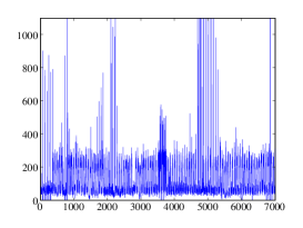
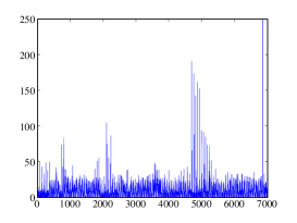
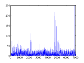
(a) - Global traffic	(b) - Traffic in monitor 1	(c) - Traffic in monitor 2
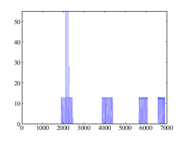
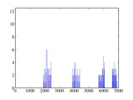
(d) - Attacks	(e) - Attacks in monitor 1	(f) - Attacks in monitor 2

Figure 1: Number of TCP/SYN packets globally exchanged (top) and received by the 4 attacked IP addresses (bottom) in the original data (a,d) and within two particular monitors (b, c, e, f). Note that the scale of the bottom figures is divided by 20 with respect to the top ones.

We consider the data used in Section 4 of Lévy-Leduc and Roueff, (2009), which corresponds to a recording of 118 minutes of ADSL (Asymmetric Digital Subscriber Line) and Peer-to-Peer (P2P) traffic to which some TCP/SYN flooding type attacks have been added. As this data set does not contain full routing information, it has been artificially distributed over a set of virtual monitors as follows: the data is shared among $K=15$ monitors by assigning each source destination pair (source IP address, destination IP address) to a randomly chosen monitor; a single monitor thus records all the flows between two particular IP addresses. The experiments reported below are based on 50 independent replication of this process. Finally, the existing anomalies have been down-sampled (by randomly dropping packets involved in the attacks) to 12.5 and 25 packets/s, respectively, to explore more difficult detection scenarios.

Figure 1-(a) displays the total number of TCP/SYN packets received during each second by the different requested IP addresses. The number of TCP/SYN packets received by the four attacked destination IP addresses are displayed in (d) (12.5 packets/s case). As we can see from this figure, the first attack occurs at around 2000 seconds, the second at around 4000 seconds, the third at around 6000 seconds and the last one at around 6500 seconds. These attacks produce 33 ground-truth anomalies – abrupt increase or decrease of the signal. Figures 1-(b), (c) display the number of TCP/SYN packets globally exchanged within two different monitors whereas (e), (f) focus on the traffic received by the attacked IP addresses within these two monitors.

The attacked IP addresses (bottom part of Figure 1) are completely hidden in the global TCP/SYN traffic (top part of Figure 1) and thus very difficult to detect. Note also that 1006000 destination IP addresses are present in this data set, with an average of 15000 destination IP addresses in each of the 118 one-minute observation windows. Hence, real time processing of the data would not be possible, even at the monitor level, without a dimension reduction step such as record filtering.

3.2 Performance of the methods

In what follows, the DTopRank algorithm is used with the same parameters as those adopted in Lévy-Leduc and Roueff, (2009) for the TopRank algorithm, with one-minute windows divided in $P=60$ subintervals of $\Delta=1$ s, with $M=10$ and $S=60$. The parameter $d$ was set to $d=1$, due to the limited number of attacks expected in each one minute window. In setting $P$ and $\Delta$ the main concern is the overall observation duration $\Delta\times P$ which should be sufficient to allow for meaningful statistical decisions while ensuring an acceptable detection delay and that the extracted series can still be considered as stationary in the absence of change. Note that the computational cost of the procedure also scales proportionally to $P$. The influence of the other parameters ($d$, $M$ and $S$) is discussed at the end of Section 4.2.

Figure 2 and 3 show the benefits of the aggregation stage within the collector of the DTopRank algorithm with respect to the use of the simple Bonferroni correction in the BTopRank algorithm. Figures 2-(a),(b) and (c) display the time series $(\underline{X}(t),\;t=1,\dots,P)$ and $(\overline{X}(t),\;t=1,\dots,P)$ associated to an attacked IP address in three different monitors as well as the corresponding $p$-values. Figure 2-(d) displays the aggregated time series $(\underline{Z}(t),\;t=1,\dots,P)$ and $(\overline{Z}(t),\;t=1,\dots,P)$, as defined in (4), as well as the associated $p$-value. Note that the aggregated time series corresponds to the aggregation of 11 time series created by 11 different monitors where the attacked IP address has been detected. The $p$-value of the aggregated time series is much smaller than the ones determined at the local monitors, which enables the detection of an attack which would be difficult to detect within the local monitors.

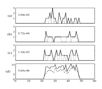
Figure 2: (a), (b), (c): times series $(\underline{X}_{i}^{(k)}(t),\;t=1,\dots,60)$ and $(\overline{X}_{i}^{(k)}(t),\;t=1,\dots,60)$ displayed with (’x’) and (’o’) respectively, for 3 different values of $k$, (d): $(\underline{Z}_{i}(t),\;t=1,\dots,60)$ and $(\overline{Z}_{i}(t),\;t=1,\dots,60)$ displayed with (’x’) and (’o’) respectively.

Figure 3 displays on the $x$ and $y$-axes the quantities $\textrm{Pval}_{\textrm{DTop}}$ and $\textrm{Pval}_{\textrm{BTop}}$, respectively. For a given IP address, $\textrm{Pval}_{\textrm{DTop}}$ corresponds to the $p$-value computed with the DTopRank and $\textrm{Pval}_{\textrm{BTop}}$ is obtained by applying the Bonferroni correction to the $p$-values transmitted by the monitors. The DTopRank provides smaller $p$-values than the Bonferroni approach for IP addresses that were really attacked and $p$-values of the same order as $\inf_{1\leq k\leq K}\textrm{Pval}_{k}$ for the other IP addresses.

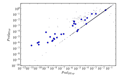
Figure 3: $(\textrm{Pval}_{\textrm{DTop}},\textrm{Pval}_{\textrm{BTop}})$ displayed with (’.’) except for the ground-truth attacked IP addresses which are displayed with (’$\bullet$’).

The DTopRank and BTopRank algorithms are further compared in Figure 4 which displays the ROC curves obtained using these two methods with 50 Monte-Carlo replications in two different cases. The bottom plot deals with attacks having an intensity of 12.5 SYN/s. In the other situation, the attacks are the same except that their intensity is 25 SYN/s. For comparison purpose, the ROC curve associated to the non distributed TopRank algorithm is also displayed in both situations. Figure 4 shows that for the 25 SYN/s-attacks, the three methods give similar results. However, in the most difficult case of the 12.5 SYN/s-attacks, the DTopRank algorithm outperforms the BTopRank algorithm.

Thus, DTopRank performs very similarly to the centralized algorithm, especially in the range of interest where the false alarm rate is about 1e-4 (recall that there are about 15000 different IP addresses in each one minute window). The quantity of data exchanged within the network is however much reduced as the centralized algorithm needs to obtain information about, on average, 34000 flows per minute whereas the DTopRank algorithm only need to transmit the $d$ upper and lower censored time series from the monitors to the collector. For $d=1$ and $K=15$, this amounts to 1800 scalars that need to be transmitted the collector, versus $34000\times 5$ (start and end time stamps, source and destination IP, number of SYN packets for each flow) for the centralized algorithm, resulting in a reduction of almost two orders of magnitude of the data that needs to be transmitted over the network.

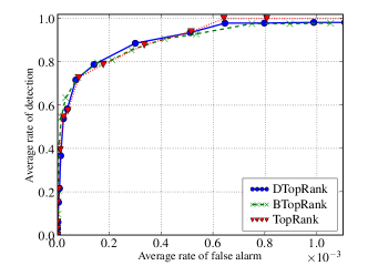
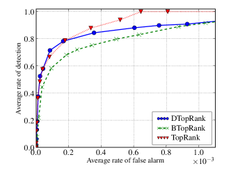
Figure 4: ROC curves for the DTopRank, BTopRank and TopRank algorithms for attacks having intensities of 25 SYN/s (top) and 12.5 SYN/s (bottom).

4 Application to synthetic data

In this section, we provide results obtained on simulated data with two specific goals in mind. First, the the traffic trace used in Section 3 contains generated attacks but is not fully labeled. Hence, it could be the case that non-labeled anomalies are already present in the background ADSL and P2P traffic contributing to a slight overestimation of false alarms (see Lévy-Leduc and Roueff, , 2009). Second, the random decentralization approach used in Section 3 does not necessarily correspond to a realistic network topology. In this section, we thus consider synthetic high-dimensional data corresponding to an idealized minute of traffic containing a single anomaly, as measured by 15 monitors randomly positioned on a plausible network topology.

4.1 Description of the data

A network topology is generated in which synthesized traffic between hosts located in the nodes of that network is injected. We first generate an Erdős-Rényi random graph (Erdős and Rényi, (1959)) with 15 nodes and a probability of edge creation of $0.15$. The generated graph is displayed in Figure 5. It is similar in terms of number of nodes or nodes degrees to the Abilene network, which has been widely considered in the context of network anomaly detection, see Lakhina et al., (2004) and Huang et al., (2007). This graph has been generated once and is used for all replications of the Monte-Carlo simulations that will follow. For each Monte-Carlo replication, a node of the graph is randomly assigned to each of the $D=1000$ IP addresses and $K=15$ monitors are also randomly positioned on 15 of the 24 edges of the graph, see Figure 5.

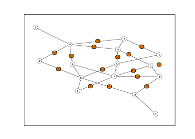
Figure 5: Generated graph: nodes are displayed with circled numbers and monitors with colored boxes.

Using the shortest path Dijkstra, (1959) algorithm, the routes between each node of the network are computed, that is the lists of edges of the graph that form the path between the nodes. These routes are used to determine which monitors will see the traffic between two hosts. Note that in our procedure, we have deliberately not considered network links capacity, that would otherwise imply some more sophisticated dynamic routing algorithms, which is beyond the scope of this contribution.

The traffic injected in this network is generated as follows. For a given Source-Destination IP address pair $(i,j)$, we follow Lévy-Leduc and Roueff, (2009) and model the SYN packet traffic using a Poisson point process with a given intensity $\theta_{i,j}$, expressed as the number of SYN packets received by $j$ per sub-interval of the observation window. In Network applications, different Source-Destinations pairs exchange a very different amount of traffic. Hence we shall use different intensities for each pair of hosts. To take into account this diversity, we propose using the realizations of a Pareto distribution for the parameters of the different intensities so that a lot of machines receive a small number of SYN packets while a few receive a lot. Note that Nucci et al., (2005) similarly use a heavy-tailed distribution to generate network traffic.

We first randomly generate a sequence $(\mu_{k})_{1\leq k\leq N}$ of intensities with the Pareto distribution having the following density: $\gamma\alpha/(1+\gamma x)^{1+\alpha}$, when $x>0$, with $\alpha=2.5$ and $\gamma=0.72$, which roughly corresponds to what we observed in the (centralized) real traffic traces used in Section 4. The parameters $\mu_{k}$ are assumed to be sorted as follows: $\mu_{1}\geq\dotsb\geq\mu_{N}$.

Here, $(X_{i,j}(t))_{1\leq t\leq P}$ correspond to the number of SYN packets sent by $i$ and received by $j$ in each of the $P$ sub-intervals of the observation window, where $i,j$ are in $\{1,\dotsc,D\}$. Among these $N$ time series, $N_{a}$ of them correspond to the traffic received by the attacked destination IP address $j_{0}$, which is assigned to a fixed location, in node 7, at the “edge” of the network (see Figure 5). This traffic, which is sent by source IP addresses $i$ belonging to a randomly chosen subset $\mathcal{I}_{a}$ of $\{1,\dotsc,D\}$, is generated as follows:

$$\forall i\in\mathcal{I}_{a},(X_{i,j_{0}}(t))_{1\leq t\leq\tau}\stackrel{{\scriptstyle iid}}{{\sim}}\textrm{Poisson}(\theta_{i,j_{0}})\;,$$

and

$$\forall i\in\mathcal{I}_{a},(X_{i,j_{0}}(t))_{\tau<t\leq P}\stackrel{{\scriptstyle iid}}{{\sim}}\textrm{Poisson}(\eta\theta_{i,j_{0}})\;,$$

where $\eta$ is a positive number which modulates the change intensity, $\tau$ is the change-point instant and $(\theta_{i,j_{0}})_{i\in\mathcal{I}_{a}}$ are chosen in $(\mu_{k})_{40N_{a}\leq k\leq 41N_{a}}$. $(\theta_{i,j_{0}})_{i\in\mathcal{I}_{a}}$ are thus chosen around 0.6 (0.4-quantile of the Pareto distribution with parameters $\alpha$ and $\gamma$, whose mean is about 0.93). Hence, the attack to be detected consists of a multiplicative increase in intensity of $N_{a}$ attacker sources, whose intensity is otherwise in the bulk of the distribution of the intensity (close to the 0.4-quantile). The remaining background traffic is generated as:

$$\forall i\in\{1,\dots,D\},\;j\neq j_{0},\;(X_{i,j}(t))_{1\leq t\leq P}\stackrel{{\scriptstyle iid}}{{\sim}}\textrm{Poisson}(\theta_{i,j})\;,$$

where $(\theta_{i,j})_{i\in\{1,\dotsc,D\},j\neq j_{0}}$ are chosen randomly in the remaining values of $\mu_{k}$: $(\mu_{k})_{k\notin[40N_{a};41N_{a}]}$.

In the experiments below, $N=10100$, $N_{a}=100$, $P=60$, $\tau=30$ and we consider different values for the parameter $\eta$ ($1.2,1.5$) in order to modulate the detection difficulty. Results presented in Figures 6 to 7 correspond to the case where $d=1$ and the influence of $d$ on the performance is discussed in the final paragraph of Section 4.2. With these settings, the DDoS-type attacks against $j_{0}$ are generated by a large number $N_{a}$ of source hosts coming from all routing nodes in in the network. Hence, these attacks can be locally (within a monitor) very difficult to distinguish from the background traffic, as can be seen in Figure 6: It displays for each monitor, when $\eta=1.5$, an example of the time series formed by the number of packets received by the first (“$\times$”) and 10th (“$\bullet$”) most solicited destination IP address at each sub-interval as well as the time series of the attacked address $j_{0}$ (“$\triangleright$”). The monitors that have not detected any traffic directed to $j_{0}$ were omitted. In (d), (e) and (i), $j_{0}$ is detected by the monitor, but the number of packets is never high enough to be selected by the record filtering step and to appear in $\{\mathcal{T}_{M}(t),\;t=1,\dotsc,60\}$. Hence in these monitors, no change detection test is performed for $j_{0}$. In the other six figures, all steps of the TopRank algorithm are carried out since the number of packets sent to $j_{0}$ is high enough. A special case is shown in (a), which displays the time series in the monitor located on the edge between nodes 10 and 7, see Figure 5, which is the link where all the traffic directed to the attacked IP address $j_{0}$ appears.

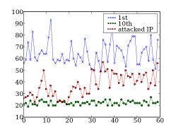
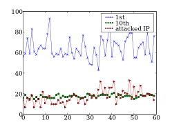
(a)	(b)	(c)
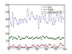
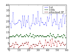
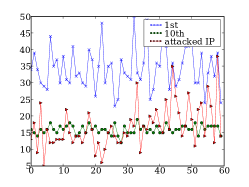
(d)	(e)	(f)
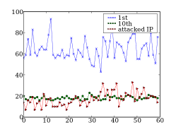
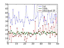
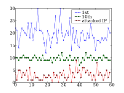
(g)	(h)	(i)

Figure 6: Time series formed in 9 monitors by the number of packets received by the first (“$\times$”) and 10th (“$\bullet$”) most solicited destination IP address at each sub-interval, as well as the time series of the attacked address $j_{0}$ (“$\triangleright$”).

4.2 Performance of the methods

The two methods described in Section 2 are compared by computing their false alarm and detection rates when tested on 1000 Monte-Carlo replications of the synthetic data described in Section 4.1. The left plot of Figure 7 displays the corresponding ROC curves for different values of $\eta$ (1.2 and 1.5); the solid and dashed lines show the results of the DTopRank and BTopRank algorithms, respectively.

For larger values of $\eta$ (1.5), both methods perform very well, with a few missed attacks for a low false alarm rate. DTopRank yields slightly better results than the other method. For $\eta=1.2$ for which attacks are more difficult to detect, the detection performance is naturally lower for both algorithms; the toll is however heavier on BTopRank than on DTopRank.

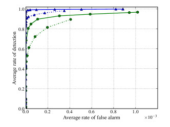
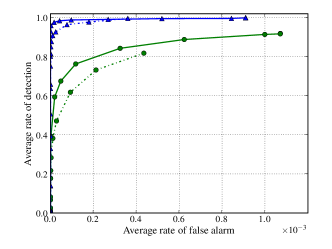
Figure 7: Left: ROC curves for DTopRank (solid lines) and BTopRank (dashed lines), for $\eta=1.2$ (“$\bullet$”), $1.5$ (“$\blacktriangle$”). Right: similar simulation when forbidding the 10-7 edge from the monitors.

We observed that the detection performance was improved for Monte Carlo runs in which a monitor is assigned to the 7–10 edge of Figure 5. Indeed in this case, at least a monitor has access to all the traffic sent to the attacked IP address sitting at node $j_{0}=7$. The right plot of Figure 7 corresponds to the case where this configuration is avoided in the Monte Carlo simulation, which gives some idea of the significance of the phenomenon. For a given monitor topology, the detection performance is thus better for target addresses located at the edge of the network, behind a monitor. In the opposite case however, the detection performance is still appreciable due to the aggregation, at the collector level, of the information sent by the monitors.

We now consider the influence of the parameter $d$ on the performance of DTopRank. Figure 8 displays the ROC curves associated to the DTopRank algorithm for different values of $d$ ($d$=1, 5, 10) and a varying number of attacks per observation window. From this figure, one can first observe from the leftmost plot that using $d=1$ for the DTopRank algorithm is optimal when there is at most one attack per window but is comparatively less advantageous as the number of attacks per window increases. Indeed, the collector then receives the time series associated to, at most, one IP address per monitor, yielding low detection rates. Increasing the value of $d$ thus improves the performance of the DTopRank algorithm when several attacks occur in the same window. However, the rightmost plot of Figure 8 reveals a form of plateauing and $d=5$ appears to provide the best tradeoff, even in cases where the actual number of attacks to be detected per window is larger than 5. This behavior can be explained by the observation that the traffic directed towards a particular attacked IP address is not always visible by all local monitors.

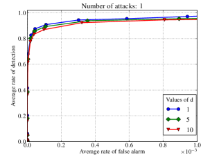
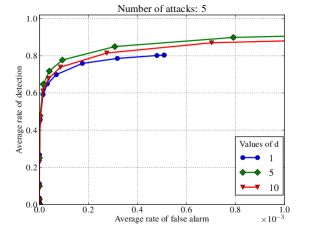
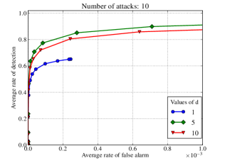
Figure 8: ROC curves for the DTopRank algorithm when the number of attacks per observation window is 1, 5, 10 (from left to right) and when $d$ equals to 1 (“$\bullet$”), 5 (“$\blacklozenge$”), 10 (“$\blacktriangledown$”).

We have also investigated how the parameters $M$ and $S$ (see Section 2.1.1) affect the performance of the DTopRank algorithm. Figure 9 shows the impact of $M$ while keeping $S$ constant to the value of $60$; both the number of attacks per observation window and the parameter $d$ were set to 5. Similar experiments, whose results are not reported here, have also shown that changing $S$ to values of 30 or 120 does not affect at all the ROC curves. From Figure 9, one can observe that larger values of $M$ consistently yield improved results, which is related to a lower censorship. Recall however that both the computational cost and the memory footprint within each monitor are proportional to $M$. Hence, the choice of $M$ results from a tradeoff between performance and memory or CPU-consumption. The absence of influence of $S$ may be explained by the fact that only $d$ values are sent to the central collector by the monitor. It suffices that $S$ be much larger than $d$ and of the order of $P$ so as to record all the “heavy hitters” that correspond to the largest $N_{i}(t)$, for all $t\in\{1,\dotsc,P\}$.

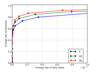
Figure 9: ROC curves for the DTopRank algorithm when the parameter $M$ takes the values of 5 (“$\bullet$”), 10 (“$\blacklozenge$”) or 20 (“$\blacktriangledown$”).

5 Conclusion

In this paper, we proposed a distributed method for detecting and localizing DDoS attacks in Internet traffic. With this approach, a local processing based on a record filtering technique followed by a nonparametric rank test is performed within the local monitors. Only the censored time series of IP addresses corresponding to the smallest $p$-values are transmitted and aggregated in the collector. The central decision, at the collector level, is based on a non-parametric change-point test for two way censored data. The processing carried out both in the monitors and in the central collector is sufficiently simple to make real-time implementations possible. The proposed algorithm has been shown to reveal attacks which are not locally detectable. Indeed, the statistical performance of the DTopRank algorithm is close to that achieved by the fully centralized detector but with a greatly reduced communication overhead. An additional interesting feature of the proposed aggregation and detection mechanism is the fact that it operates similarly at the monitor and collector level. Hence, the test could also be applied hierarchically, with tree structured monitors, so as to produce decisions corresponding to groups of monitors of different granularity in the network.

Appendix A Appendix

A.1 Proof of Theorem 1

The following proof is based on (Billingsley, , 1968, Theorem 24.2), which asserts that if $\xi_{1},\dotsc,\xi_{n}$ are exchangeable random variables (each permutation of the set of variables has the same joint distribution) and satisfy, as $n\rightarrow\infty$,

$$\sum_{i=1}^{n}\xi_{i}\stackrel{{\scriptstyle p}}{{\longrightarrow}}0,\quad\sum_{i=1}^{n}\xi^{2}_{i}\stackrel{{\scriptstyle p}}{{\longrightarrow}}1,\quad\max_{1\leq i\leq n}|\xi_{i}|\stackrel{{\scriptstyle p}}{{\longrightarrow}}0\;,$$ (5)

then $\{\sum_{i=1}^{\lfloor nt\rfloor}\xi_{i}\;,0\leq t\leq 1\}\stackrel{{\scriptstyle d}}{{\longrightarrow}}\{B(t)\;,\;0\leq t\leq 1\}$, as $n\rightarrow\infty$, where $B$ is a Brownian bridge.

We apply this theorem to the random variables $Y_{1},\dotsc,Y_{P}$, defined in (1), which are exchangeable since $(\underline{X}(i),\overline{X}(i))_{1\leq i\leq P}$ are i.i.d random vectors. Let us now check the three conditions in (5). By the anti-symmetry of the kernel $h$,

$$\sum_{i=1}^{P}U_{i}=\sum_{i=1}^{P}\sum_{j=1}^{P}h(i,j)=0\;,$$

which gives the first condition of the theorem. The second one follows from the definition of $Y_{i}$:

$$\sum_{i=1}^{p}Y_{i}^{2}=\frac{1}{\sum_{j=1}^{p}U^{2}_{j}}\sum_{i=1}^{p}U_{i}^{2}=1\;.$$

To check the third condition, denote by $F_{P}$ (resp. $G_{P}$) the empirical c.d.f. of $\overline{X}(1),\dotsc,\overline{X}(P)$ (resp. $\underline{X}(1),\dotsc,\underline{X}(P)$):

$$F_{P}(t)=P^{-1}\sum_{i=1}^{P}\mathbf{1}(\overline{X}(i)\leq t)\textrm{ and }G_{P}(t)=P^{-1}\sum_{i=1}^{P}\mathbf{1}(\underline{X}(i)\leq t)\;.$$ (6)

Note that

$$\frac{1}{P}U_{i}=\frac{1}{P}\sum_{j=1}^{P}\mathbf{1}(\underline{X}(i)>\overline{X}(j))-\mathbf{1}(\overline{X}(i)<\underline{X}(j))\\ =F_{P}(\underline{X}(i)^{-})-\{1-G_{P}(\overline{X}(i))\}=F_{P}(\underline{X}(i)^{-})-\overline{G}_{P}(\overline{X}(i))\;,$$ (7)

where $\overline{G}_{P}(\cdot)=1-G_{P}(\cdot)$. Then, using the Glivenko-Cantelli Theorem (van der Vaart, , 1998, Theorem 19.1), we get, as $P$ tends to infinity, that

$$\frac{1}{P}\sum_{j=1}^{P}\left(\frac{1}{P}U_{j}\right)^{2}\\ =\frac{1}{P}\sum_{j=1}^{P}F_{P}(\underline{X}(i)^{-})^{2}-\frac{2}{P}\sum_{j=1}^{P}F_{P}(\underline{X}(i)^{-})\overline{G}_{p}(\overline{X}(i))+\frac{1}{P}\sum_{j=1}^{P}\overline{G}_{p}(\overline{X}(i))^{2}\\ =\frac{1}{P}\sum_{j=1}^{P}F(\underline{X}(i)^{-})^{2}-\frac{2}{P}\sum_{j=1}^{P}F(\underline{X}(i)^{-})\overline{G}(\overline{X}(i))+\frac{1}{P}\sum_{j=1}^{P}\overline{G}(\overline{X}(i))^{2}+o_{p}(1)\;.$$

By the law of large numbers and our assumption in (2), we obtain, as $P$ tends to infinity, that

$$\frac{1}{P}\sum_{j=1}^{P}\left(\frac{1}{P}U_{j}\right)^{2}\stackrel{{\scriptstyle p}}{{\longrightarrow}}\mathbb{E}[\{F(\underline{X}^{-})-\overline{G}(\overline{X})\}^{2}]>0\;.$$ (8)

Using (7), $P^{-1}|U_{i}|\leq 2$, $i=1,\dotsc,P$, and thus

$$|Y_{i}|=\frac{|U_{i}|}{\sqrt{\sum_{j=1}^{P}U^{2}_{j}}}=\frac{1}{\sqrt{P}}\frac{P^{-1}|U_{i}|}{\sqrt{P^{-1}\sum_{j=1}^{P}(P^{-1}U_{j})^{2}}}\\ \leq\frac{1}{\sqrt{P}}\frac{2}{\sqrt{P^{-1}\sum_{j=1}^{P}(P^{-1}U_{j})^{2}}}\;,\;i=1,\dots,P\;.$$

By (8), $Y_{i}$ satisfies the third condition of (5), which completes the proof.

References

- Basseville and Nikiforov, (1993) Basseville, M. and Nikiforov, I. V. (1993). Detection of Abrupt Changes: Theory and Applications. Prentice-Hall.
- Billingsley, (1968) Billingsley, P. (1968). Convergence of probability measures. Wiley, New York.
- Brodsky and Darkhovsky, (1993) Brodsky, B. E. and Darkhovsky, B. S. (1993). Nonparametric Methods in Change-Point Problems. Kluwer Academic Publisher.
- Csörgő and Horváth, (1997) Csörgő, M. and Horváth, L. (1997). Limit theorems in change-point analysis. Wiley, New-York.
- Dijkstra, (1959) Dijkstra, E. (1959). A note on two problems in connexion with graphs. Numerische mathematik, 1(1):269–271.
- Erdős and Rényi, (1959) Erdős, P. and Rényi, A. (1959). On random graphs. I. Publ. Math. Debrecen, 6:290–297.
- Gombay and Liu, (2000) Gombay, E. and Liu, S. (2000). A nonparametric test for change in randomly censored data. The Canadian Journal of Statistics, 28(1):113–121.
- Huang et al., (2007) Huang, L., Nguyen, X., Garofalakis, M., Jordan, M. I., Joseph, A., and Taft, N. (2007). In-network pca and anomaly detection. In Schölkopf, B., Platt, J., and Hoffman, T., editors, Advances in Neural Information Processing Systems 19, pages 617–624. MIT Press, Cambridge, MA.
- Krishnamurthy et al., (2003) Krishnamurthy, B., Sen, S., Zhang, Y., and Chen, Y. (2003). Sketch-based change detection: methods, evaluation, and applications. In IMC ’03: Proceedings of the 3rd ACM SIGCOMM conference on Internet measurement, pages 234–247, New York, NY, USA. ACM.
- Lakhina et al., (2004) Lakhina, A., Crovella, M., and Diot, C. (2004). Diagnosing network-wide traffic anomalies. In SIGCOMM ’04: Proceedings of the 2004 conference on Applications, technologies, architectures, and protocols for computer communications, pages 219–230, New York, NY, USA. ACM.
- Lévy-Leduc and Roueff, (2009) Lévy-Leduc, C. and Roueff, F. (2009). Detection and localization of change-points in high-dimensional network traffic data. Annals of Applied Statistics, 3(2):637–662.
- Nucci et al., (2005) Nucci, A., Sridharan, A., and Taft, N. (2005). The problem of synthetically generating IP traffic matrices: initial recommendations. ACM SIGCOMM Computer Communication Review, 35(3):19–32.
- Park et al., (2005) Park, C., Hernandez-Campos, F., Marron, J., and Smith, F. D. (2005). Long-range dependence in a changing internet traffic mix. Computer Networks, 48(3):401 – 422.
- Siris and Papagalou, (2006) Siris, V. A. and Papagalou, F. (2006). Application of anomaly detection algorithms for detecting syn flooding attacks. Computer Communications, 29(9):1433 – 1442. ICON 2004 - 12th IEEE International Conference on Network 2004.
- Susitaival et al., (2006) Susitaival, R., Juva, I., Peuhkuri, M., and Aalto, S. (2006). Characteristics of origin-destination pair traffic in funet. Telecommunication Systems, 33:67–88.
- Tartakovsky et al., (2006) Tartakovsky, A., Rozovskii, B., Blazek, R., and Kim, H. (2006). Detection of intrusion in information systems by sequential change-point methods. Statistical Methodology, 3(3):252–340.
- van der Vaart, (1998) van der Vaart, A. W. (1998). Asymptotic statistics, volume 3 of Cambridge Series in Statistical and Probabilistic Mathematics. Cambridge University Press, Cambridge.
- Wang et al., (2002) Wang, H., Zhang, D., and Shin, K. G. (2002). Detecting syn flooding attacks. INFOCOM 2002. Twenty-First Annual Joint Conference of the IEEE Computer and Communications Societies. Proceedings. IEEE, 3:1530–1539.