Comparison between scattering-states numerical renormalization group and the Kadanoff-Baym-Keldysh approach to quantum transport: Crossover from weak to strong correlations

Abstract

The quantum transport through nanoscale junctions is governed by the charging energy $U$ of the device. We employ the recently developed scattering-states numerical renormalization group approach to open quantum systems to study nonequilibrium Green’s functions and current-voltage characteristics of such junctions for small and intermediate values of $U$. We establish the accuracy of the approach by a comparison with diagrammatic Kadanoff-Baym-Keldysh results which become exact in the weak coupling limit $U\to 0$. We demonstrate the limits of the diagrammatic expansions at intermediate values of the charging energy. While the numerical renormalization group approach correctly predicts only one single, universal low-energy scale at zero bias voltage, some diagrammatic expansions yield two different low-energy scales for the magnetic and the charge fluctuations. At large voltages, however, the self-consistent second Born as well as the GW approximation reproduce the scattering-states renormalization group spectral functions for symmetric junctions, while for asymmetric junctions the voltage-dependent redistribution of spectral weight differs significantly in the different approaches. The second-order perturbation theory does not capture the correct single-particle dynamics at large bias and violates current conservation for asymmetric junctions.

I Introduction

Quantum dots and single-molecule junctions have been considered as possible building blocks for nano-electronics and quantum-information processing.Elzerman et al. (2004); Nitzan and Ratner (2003); Temirov et al. (2008) Recent technological progress has made it possible to manufacture and study electron transport trough ultra-small quantum-dot devices, nanotubes or single molecules.Goldhaber-Gordon et al. (1998a, b); van der Wiel et al. (2000); Nagaoka et al. (2002); Quay et al. (2007); Temirov et al. (2008); Grobis et al. (2008); Amasha et al. (2005); Liu et al. (2009) These devices are designed as a small central region comprising of a quantum dot or a single molecule which is coupled to at least two leads where the finite bias voltage is applied to. The investigation of such devices is of fundamental importance for our understanding of open quantum systems out of equilibrium.

Due to the quantization of the charge, the physical properties of such junctions are dominated by many-body effects at temperatures below the charging energy $U=e^{2}/(2C)$, where $C$ is the capacitance of the device. The experimental devices are often fully controllable by external gate electrodes or elongation of the scanning tunneling microscope tip.Temirov et al. (2008) This gives the opportunity to directly study true many-body correlation effects, such as the Kondo effect (see for example Ref. Hewson, 1993a and kon, 2005), under the influence of an external bias voltage. However, the theoretical understanding of the interplay between coherent transport favored by many-body correlations and current-driven dephasing at finite bias is still at its infancy and further investigations are needed.

The present work has two main objectives. On the one hand, we establish the reliability of the recently introduced scattering-states numerical renormalization group (SNRG) approachAnders (2008a) to quantum transport by comparing results for small values of $U$ to the diagrammatic Kadanoff-Baym-Keldysh approach, which becomes exact in the limit $U\to 0$. On the other hand, we will discuss discrepancies and reveal shortcomings of those diagrammatic approaches at intermediate values of the charging energy.

We investigate quantum transport through a quantum-dot device using a minimal modelWingreen and Meir (1994) where the complex interacting region is replaced by a single spinful orbital which is coupled to two noninteracting leads. A single Coulomb matrix element $U$ accounts for the charging energy of the device. We calculate nonequilibrium spectral functionsAnders (2008b) and current-voltage (IV) characteristics using the SNRG as well as different approximationsThygesen and Rubio (2007); Darancet et al. (2007); Spataru et al. (2009); Myohanen et al. (2009) within the diagrammatic Kadanoff-Baym-Keldysh expansion in the local Coulomb interaction $U$.

Over the past 40 years, the Keldysh technique Keldysh (1965) has proven to be the most successful approach to nonequilibrium dynamics. In the context of quantum transport through nano-junctions direct expansions in the interactionYeyati et al. (1993); Takagi and Saso (1999); Matsumoto (2000); Fujii and Ueda (2003) as well as self-consistent re-summation schemes have been employed.Thygesen and Rubio (2007); Darancet et al. (2007); Spataru et al. (2009); Myohanen et al. (2009) However, such diagrammatic expansions rely on a small expansion parameter, and are, therefore, confined to weak coupling. But quantum-impurity modelsBulla et al. (2008a) commonly used in the theory of quantum transport on the molecular level often exhibit infra-red divergences in perturbation theoryHewson (1993a) which also restrict the diagrammatic Keldysh approaches to certain parameter regimes usually to high temperature or to large bias.

In contrast to equilibrium conditions, where complete and accurate solutions can be obtained using a variety of nonperturbative techniques such as the Bethe ansatz,Andrei et al. (1983); Tsvelick and Wiegmann (1983) conformal field theory,Affleck and Ludwig (1991, 1993) or Wilson’s numerical renormalization group (NRG) approach,Wilson (1975); Bulla et al. (2008a) techniques for calculating quantum-transport out of equilibrium remain largely at the development stage. Recent advancements on the analytical side Kaminski et al. (2000); Rosch et al. (2001); Jakobs et al. (2007); Gezzi et al. (2007); Doyon and Andrei (2006); Mehta and Andrei (2006) include suitable adaptations of the Wegner’s flow-equationKehrein (2005, 2006) and the real-time renormalization-group method.Schoeller and Koenig (2000); Schoeller (2009); Pletyukhov et al. (2009) These methods can successfully access large voltages, but are generally confined to the weak-coupling regime. Based on the scattering-states approach to quantum transportHershfield (1993); Doyon and Andrei (2006) the Bethe ansatz was extended to quantum-impurity models out of equilibrium,Mehta and Andrei (2006) but remains limited to a certain class of models.

On the numerical side, progress has been made in several directions. Currents have been extracted from time-dependent density matrix renormalization groupSchmitteckert (2004); Schollwöck (2005); Kirino et al. (2008); Heidrich-Meisner et al. (2009) calculations using finite 1D wires, and the results agree well with Bethe ansatz results for certain models.Boulat et al. (2008) Quantum Monte Carlo approaches based on scattering statesHershfield (1993) can access the intermediate coupling regimeHan and Heary (2007); Dirks et al (2010) at finite bias. Recent real-time formulations of continuous-time quantum Monte CarloMühlbacher and Rabani (2008); Werner et al. (2009, 2010) and an iterative real-time path integral approachWeiss et al. (2008) to quantum transport offer the appealing advantage of working directly in the continuum limit, but are confined to relatively short time scales. Access to low temperatures and long times is hampered in the former case by a severe sign problem, and by the extrapolation to long memory times in the latter case. Hence neither approach can presently be applied to nonequilibrium dynamics of correlated systems with a small underlying energy scale, as is the case with ultra-small quantum dots when tuned to the Kondo regime.

The usage of Lippmann-Schwinger scattering states has been well established in quantum-field theorySchweber (1962) for over 50 years and also successfully adapted to the description of quantum transport through strongly interacting nano-devices coupled to ballistic leads.Hershfield (1993); Doyon and Andrei (2006); Han (2006); Mehta and Andrei (2006) These states fulfill the correct boundary condition of the open quantum system: (i) they break time-reversal symmetry and, therefore, are (ii) complex and current-carrying and (iii) describe ballistic transport in the leads combined with scattering events in the small interacting quantum-dot region. This time-reversal symmetry breaking is required for current carrying systems and reveals itself naturally in all diagrammatic approaches by the occurrence of retarded and advanced Green’s functions. It is a consequence of any regularization when performing the limit to an infinitely large system.

In particular, the work of Hershfield Hershfield (1993) and Doyon and Andrei Doyon and Andrei (2006) has rigorously shown that these boundary conditions remain unaltered when a local interaction is switched on. The noninteracting current-carrying system evolves into the new steady-state of the interacting system, and the steady-state density operator retains a Boltzmannian form.Hershfield (1993) The explicit construction of those scattering states allows to exactly solve the DC and AC Kondo model at the Toulouse pointSchiller and Hershfield (1995, 1996); Schiller and Hershfield (2000) as well as the interacting resonant level model.Mehta and Andrei (2006); Boulat et al. (2008)

Recently, an extensionAnders (2008a) to Wilson’s numerical renormalization group has been developed for steady-state quantum transport through nano-devices which is able to deal with the crossover from weak to strong coupling for arbitrary bias voltages. It is based on Oguri’s ideaOguri (2007) of discretizing the single-particle scattering states which are the solutions of the Lippman-Schwinger equationSchweber (1962) for the noninteracting problem and, therefore, fulfill the correct boundary condition of an open quantum system. This scattering-states numerical renormalization group approachAnders (2008a) (SNRG) evolves the analytically known density matrix of a noninteracting system to the density matrix of the fully interacting problem by employing the time-dependent NRG (TD-NRG).Anders and Schiller (2005, 2006) The NRG is ideally suited to the problem, being known to provide accurate solutions of quantum-impurity models on all relevant interaction strengths at zero bias.Bulla et al. (2008a) Since the TD-NRG can access exponentially long time scales,Anders and Schiller (2005, 2006) dwell times on the order of the inverse Kondo-temperature are easily accessible.

This paper is organized as follows. After the model used is defined, we provide the details of the different theoretical approaches in Sec. II. We summarize the basic ideas of the SNRG method introduced in Ref. Anders, 2008a in Sec. II.2 and state all necessary equations of the diagrammatic nonequilibrium techniques in Sec. II.3. The main body of the paper is in Sec. III, where we present and discuss the results obtained for the various methods. In order to set the stage for a detailed comparison between the SNRG and diagrammatic approaches at finite bias, we begin with a discussion of the magnetic and charge fluctuation scales at zero bias in Sec. III.1. Since the NRG provides an accurate solution in this regime for arbitrary coupling strengths and temperatures, this reveals the validity range of the diagrammatic approaches. We show that — in contrast to the NRG — some of the diagrammatic expansions fail to produce a single low-energy scale for intermediate and large values of $U$. However, in the weak correlation regime all these approaches agree excellently for arbitrary voltages at small $U$ and yield the same nonequilibrium Green functions as well as IV characteristics which are presented in Sec. III.2. Discrepancies between the different approaches at intermediate values of the Coulomb interaction are discussed in Sec. III.3, where the spectral functions and IV curves of a symmetric and an asymmetric junction are considered. We conclude with summary and a short outlook in Sec. IV.

II Theory

II.1 Model

Quantum impurity models are used to describe quantum transport on the molecular level. Their Hamiltonian ${\cal H}$

$${\cal H} = {\cal H}_{imp}+{\cal H}_{bath}+{\cal H}_{I}$$ (1)

consists of three parts: an impurity part ${\cal H}_{imp}$ modeling the interacting device with a finite number of degrees of freedom, one or several bosonic or fermionic baths represented by ${\cal H}_{bath}$, and the coupling of these subsystems by ${\cal H}_{I}$.

Throughout this paper, we restrict ourselves to junctions modeled by the single impurity Anderson model with one spinful orbital coupled to a left (L) and a right (R) lead and an on-site Coulomb repulsion $U$

$${{\cal H}} = \sum_{\sigma\alpha=L,R}\int d\epsilon\,(\epsilon-\mu_{\alpha})\,c^{\dagger}_{\epsilon,\sigma\alpha}c_{\epsilon,\sigma\alpha}$$ (2)

$$+\sum_{\sigma=\pm 1}E_{d}\>\hat{n}^{d}_{\sigma}+U\hat{n}^{d}_{\uparrow}\hat{n}^{d}_{\downarrow}$$

$$+\sum_{\alpha\sigma}t_{\alpha\sigma}\int d\epsilon\,\sqrt{\rho_{\alpha}(\epsilon)}\left\{d^{\dagger}_{\sigma}c_{\epsilon\sigma\alpha}+c^{\dagger}_{\epsilon\sigma\alpha}d_{\sigma}\right\}.$$

Here, $E_{d}$ is the single-particle energy of the quantum dot, $\hat{n}_{\sigma}^{d}=d^{\dagger}_{\sigma}d_{\sigma}$ measures its orbital occupancy and $t_{\alpha\sigma}$ represent the elementary hybridization-matrix elements coupling the dot to the two leads. The different chemical potentials $\mu_{\alpha}$ in both leads appear as a shift of the band centers and are functions of the external voltage $V=\mu_{R}-\mu_{L}$.

For simplicity, we assume that both leads have the same density of states, $\rho_{R}(\epsilon)=\rho_{L}(\epsilon)\equiv\rho(\epsilon)$, characterized by the same band width $D$ but different band centers. This Hamiltonian is commonly used to model a single Coulomb-blockade resonance in ultra-small quantum dots.Wingreen and Meir (1994); Goldhaber-Gordon et al. (1998a)

II.2 Scattering-states numerical renormalization group approach

II.2.1 Definition of the scattering states

In the absence of the local Coulomb repulsion $H_{U}=U\hat{n}^{d}_{\uparrow}\hat{n}^{d}_{\downarrow}$, the single-particle problem is diagonalized exactly in the continuum limitHan (2006); Hershfield (1993); Enss et al. (2005); Han and Heary (2007); Oguri (2007); Lebanon et al. (2003); Anders (2008a) by the following scattering-states creation operators

$$\gamma^{\dagger}_{\epsilon\sigma\alpha} = c^{\dagger}_{\epsilon\sigma\alpha}+t_{\alpha}\sqrt{\rho_{\alpha}(\epsilon)}G_{0\sigma}^{r}(\epsilon)\Bigg{[}d^{\dagger}_{\sigma}$$ (3)

$$+\sum_{\alpha^{\prime}}\int d\epsilon^{\prime}\frac{t_{\alpha^{\prime}}\sqrt{\rho_{\alpha^{\prime}}(\epsilon^{\prime})}}{\epsilon+i\delta-\epsilon^{\prime}}c^{\dagger}_{\epsilon^{\prime}\sigma\alpha^{\prime}}\Bigg{]}\;\;.$$

$\alpha=L(R)$ labels left (right) moving scattering states created by $\gamma^{\dagger}_{\epsilon\sigma L(R)}$. The local retarded resonant level Green’s function

$$G^{r}_{0\sigma}(\omega) = \left[\omega+i\delta-E_{d}-\sum_{\alpha}t^{2}_{\alpha}\int d\epsilon\frac{\rho_{\alpha}(\epsilon)}{\omega+i\delta-\epsilon}\right]^{-1}$$ (4)

enters as an expansion coefficient. Defining $\bar{t}=\sqrt{t_{L}^{2}+t_{R}^{2}}$, we will use $r_{R(L)}=t_{R(L)}/\bar{t}$ and

$$\Delta(\omega) = \bar{t}^{2}\sum_{\alpha}r^{2}_{\alpha}\int d\epsilon\frac{\rho_{\alpha}(\epsilon)}{\omega+i\delta-\epsilon}$$ (5)

$$= \Re e[\Delta(\omega)]-i\Gamma(\omega)$$

in the following.

In the limit of infinitely large leads — volume $Vol.\to\infty$ — the single-particle spectrum remains unaltered, and these scattering states diagonalize the Hamiltonian (2) for $U=0$:

$${\cal H}^{i}_{0}={\cal H}(U=0) = \sum_{\alpha=L,R;\sigma}\int d\epsilon\,\epsilon\gamma^{\dagger}_{\epsilon\sigma\alpha}\gamma_{\epsilon\sigma\alpha}\;\;.$$ (6)

The scattering states are solutions of the Lippmann-Schwinger equationSchweber (1962) and therefore break time-reversal symmetry, which constitutes a necessary boundary condition to describe a current carrying open quantum system. This is encoded in the small imaginary part $+i\delta$ entering Eq. (3) – (5) required for convergence when performing the continuum limit $Vol.\to\infty$ in the leads.

The complex expansion coefficients in (3) are given by retarded functions, e.g. $G_{0\sigma}^{r}(\epsilon)$, which causes the scattering states to be complex and current carrying. For zero bias voltage, time-reversal symmetry manifests itself in the identical spectrum for left and right movers which are time-reversal pairs in that limit.

To avoid any contribution from bound states, we will implicitly assume a wide band limit: $D\gg max\{|E_{d}|,\Gamma,|V|\}$, where $\Gamma_{\alpha}=\pi t_{\alpha}^{2}\rho(0)$ and $\Gamma=\Gamma_{L}+\Gamma_{R}$.

Hershfield has shown that the density operator for such a noninteracting current carrying quantum system retains its Boltzmannian formHershfield (1993)

$$\hat{\rho}_{0} = \frac{e^{-\beta({\cal H}^{i}_{0}-\hat{Y}_{0})}}{\textrm{Tr}\left[e^{-\beta({\cal H}^{i}_{0}-\hat{Y}_{0})}\right]}\,,\,\hat{Y}_{0}=\sum_{\alpha\sigma}\mu_{\alpha}\int d\epsilon\,\gamma^{\dagger}_{\epsilon\sigma\alpha}\gamma_{\epsilon\sigma\alpha}$$ (7)

even for finite bias. The $\hat{Y}_{0}$ operator accounts for the different occupation of the left- and right-moving scattering states, and $\mu_{\alpha}$ for the different chemical potentials of the leads.

Therefore, all steady-state expectation values of operators can be calculated using $\hat{\rho}_{0}$ which includes the finite bias. In the absence of a Coulomb repulsion $U$, this is a trivial and well-understood problem. It was shownOguri (2007) that the current expectation value using this density-operator $\hat{\rho}_{0}$ reproduced the standard resultHershfield et al. (1991a); Meir and Wingreen (1992a); Wingreen and Meir (1994) for noninteracting devices. The knowledge of the analytical form of $\hat{\rho}_{0}$, however, makes this steady-state model accessible to a NRG approach.Bulla et al. (2008a); Anders (2008a)

The expansion coefficients of $\gamma^{\dagger}_{\epsilon\sigma\alpha}$ in Eq. (3) contain the complex single-particle Green function $G_{0\sigma}^{r}(\epsilon)$ which we separate in modulus and phase

$$G_{0\sigma}^{r}(\epsilon) = |G_{0\sigma}^{r}(\epsilon)|e^{-i\Phi_{\sigma}(\epsilon)}\quad.$$ (8)

This phase is absorbed into the new scattering states $\gamma^{\dagger}_{\epsilon\sigma\alpha}\to\tilde{\gamma}^{\dagger}_{\epsilon\sigma\alpha}=\gamma^{\dagger}_{\epsilon\sigma\alpha}e^{i\Phi_{\sigma}(\epsilon)}$ by a local gauge transformation. The impurity operator $d^{\dagger}_{\sigma}$ is expanded into left- and right-mover contributions

$$d^{\dagger}_{\sigma} = r_{R}d^{\dagger}_{\sigma R}+r_{L}d^{\dagger}_{\sigma L}$$ (9)

using the inversion of Eq. (3). These two new operators $d^{\dagger}_{\sigma\alpha}$ are then defined as

$$d^{\dagger}_{\sigma\alpha} = \bar{t}\int d\epsilon\sqrt{\rho(\epsilon)}|G_{0\sigma}^{r}(\epsilon)|\tilde{\gamma}^{\dagger}_{\epsilon\sigma\alpha}\;\;,$$ (10)

and obey the anti-commutator relation $\{d_{\sigma\alpha},d_{\sigma^{\prime}\alpha^{\prime}}^{\dagger}\}=\delta_{\alpha\alpha^{\prime}}\delta_{\sigma\sigma^{\prime}}$.

II.2.2 Discretization of the scattering states

The scattering-states numerical renormalization group approachAnders (2008a) (SNRG) starts from a logarithmic discretization of the scattering-states continuum $\gamma_{\epsilon\sigma\alpha}$ in intervals $I^{n}_{+}=[\Lambda^{-(n+z)}D,\Lambda^{-(n+z-1)}D]$ and $I^{n}_{-}=[-\Lambda^{-(n+z-1))}D,-\Lambda^{-(n+z)}D]$ $(n=1,2,\cdots)$, controlled by the parametersWilson (1975); Bulla et al. (2008a) $\Lambda>1$ and $z\in(0,1]$. The intervals for $n=0$ are defined as $I^{0}_{+}=[\Lambda^{-z}D,D]$ and $I^{0}_{-}=[-D,-\Lambda^{-z}D]$. An average over various $z$-valuesYoshida et al. (1990) is used to mimic the conduction band continuum.

Then, the discretized version of the noninteracting Hamiltonian (6) is mapped onto a semi-infinite Wilson chain

$$H_{0}(\Lambda) = \sum_{\sigma\alpha}\sum_{n=0}^{\infty}w_{n\sigma\alpha}f^{\dagger}_{n\sigma\alpha}f_{n\sigma\alpha}+\sum_{\sigma\alpha}\sum_{n=0}^{\infty}\left(t_{n\sigma\alpha}f^{\dagger}_{n\sigma\alpha}f_{n+1\sigma\alpha}+t^{*}_{n\sigma\alpha}f^{\dagger}_{n+1\sigma\alpha}f_{n\sigma\alpha}\right)$$ (11)

whose tight-binding matrix elements $t_{n\sigma\alpha}$ decay exponentially $t_{n\sigma\alpha}\propto\Lambda^{-n/2}$ for large $n$. In contrast to the standard NRG,Wilson (1975); Bulla et al. (2008a) the impurity degree of freedom has been included into $H_{0}(\Lambda)$ since not the leads but the full scattering states have been discretized. Any complex phase in the tight-binding parameters $t_{n\sigma\alpha}$ can be absorbed into the creation (anihilation) operators $f^{\dagger}_{n\sigma\alpha}$ $(f_{n\sigma\alpha})$ of an electron on the chain link $n$ with spin $\sigma$ and mover $\alpha$ by a local gauge transformation.

We use $d_{\sigma\alpha}$ defined in Eq. (10) as starting vector $f_{0\sigma\alpha}=d_{\sigma\alpha}$ for the Householder transformationWilson (1975) and obtain the tight-binding coefficients of the Wilson chain (11) by the usual procedure.Wilson (1975); Bulla et al. (2008a) It is straight forward to shown that the energy of the first chain link corresponds to the energy of the original quantum-dot orbital: $w_{0\sigma\alpha}=E_{d}$.

II.2.3 Local Coulomb interaction

In order to include the local Coulomb interaction, the density operator $\hat{n}^{d}_{\sigma}=d^{\dagger}_{\sigma}d_{\sigma}$ must be expanded in the new orbitals $d_{\sigma\alpha}$. It consist of two contributions: A density term and a backscattering term $\hat{n}^{d}_{\sigma}=\hat{n}^{0}_{\sigma}+\hat{O}_{\sigma}^{back}$, where

$$\hat{n}^{0}_{\sigma} = \sum_{\alpha}r_{\alpha}^{2}d^{\dagger}_{\sigma\alpha}d_{\sigma\alpha}$$ (12)

and the backscattering $\hat{O}_{\sigma}^{back}$ term is defined as

$$\hat{O}_{\sigma}^{back} = r_{L}r_{R}\left(d^{\dagger}_{\sigma R}d_{\sigma L}+d^{\dagger}_{\sigma L}d_{\sigma R}\right).$$ (13)

The local Coulomb interaction $H_{U}$

$$H_{U} = U\left(\hat{n}^{0}_{\uparrow}\hat{n}^{0}_{\downarrow}+\sum_{\sigma}\hat{O}_{\sigma}^{back}\hat{n}^{0}_{-\sigma}+\hat{O}_{\uparrow}^{back}\hat{O}_{\downarrow}^{back}\right)$$ (14)

leads to a mixing of left and right movers since $\hat{O}_{\sigma}^{back}$ does not commute with $Y_{0}$. However, the term $H_{U}^{0}$,

$$H_{U}^{0}=\frac{U}{2}\left(\sum_{\sigma}\hat{n}^{0}_{\sigma}-1\right)^{2},$$ (15)

commutes with $\hat{Y}_{0}$ and can be absorbed into the steady-state density operator $\hat{\rho}_{0}\to\tilde{\rho}_{0}=\exp[-\beta({\cal H}^{i}-\hat{Y}_{0})]/Z$ with ${\cal H}^{i}={\cal H}^{i}_{0}+H_{U}^{0}$ using the arguments given in Ref. Doyon and Andrei, 2006.

II.2.4 Review of the time-dependent numerical renormalization group approach

Starting from an equilibrated system for times $t\leq 0$, the initial Hamiltonian ${{\cal H}_{i}}$ is changed to ${{\cal H}_{f}}$ by a sudden quench at $t=0$. Then, the density operator $\hat{\rho}(t)$ evolves from its initial value $\hat{\rho}_{0}$ at $t=0$ as

$$\hat{\rho}(t) = e^{-i{\cal H}_{f}t/\hbar}\hat{\rho}_{0}e^{i{\cal H}_{f}t/\hbar}\;\;.$$ (16)

If ${\cal H}_{i(f)}$ describes a quantum impurity problem and $\hat{O}$ is an impurity operator, it was recently shown that the real-time dynamics of the expectation value of $O(t)=\langle\hat{O}(t)\rangle$ can be calculatedAnders and Schiller (2005, 2006) by evaluating

$$O(t) = \sum_{m}\sum_{r,s}^{dis}\rho^{red}_{r,s}(m)O^{m}_{s,r}\,e^{-i(E^{m}_{r}-E_{s}^{m})t/\hbar}$$ (17)

where $O^{m}_{s,r}=\langle s,e;m|\hat{O}|r,e;m\rangle$ denotes the matrix elements of the operator $\hat{O}$ and $E^{m}_{r}$ the NRG eigenenergy of the eigenstate $|r;m\rangle$ to ${\cal H}_{f}$ at NRG iteration $m$. The sum restriction $\sum_{r,s}^{dis}$ indicates that at least one of the states $r,s$ must be a discard state at iteration $m$. Excitations between two retained states will be refined in the following iterations $m^{\prime}>m$ and, therefore, will contribute at a later iteration. $e$ labels the environment degrees of freedom of the Wilson chain links to be incorporated in subsequent iterations $m^{\prime}>m$ and the $|r,e;m\rangle=|r;m\rangle\otimes|e\rangle$ are just tensor-product states of the eigenstates of the $m$th iteration and the yet uncoupled rest chain. The reduced density matrix

$$\rho^{red}_{r,s}(m) = \sum_{e}\langle r,e;m|\hat{\rho}_{0}|s,e;m\rangle$$ (18)

traces out all environment degrees of freedom $e$. The initial conditions are encoded into the density operator $\hat{\rho}_{0}$ calculated with the initial Hamiltonian ${{\cal H}_{i}}$. The calculation of the overlap matrix between the NRG eigenstates of ${{\cal H}_{i}}$ and ${{\cal H}_{f}}$ allows for the basis set transformation of $\rho^{red}_{r,s}(m)$ into the basis of the final Hamiltonian provided that $\hat{\rho}_{0}$ remains restricted to the last Wilson shell.Anders and Schiller (2005, 2006) This transformed $\rho^{red}_{r,s}(m)$ enters Eq. (17).

The discarded states form a complete basis setAnders and Schiller (2005) for the Fock-space of the entire Wilson chain of length $N$, i.e. $\mathcal{F}_{N}=\mathrm{span}\{|l,e;m\rangle\}$ where $l$ labels all discarded states at iteration $m$. The iterative diagonalization thus procures the set of (approximate) eigenstates for the whole energy range from high energies on the order of the bandwidth down to very low energies such as the Kondo scale. This is indispensable because nonequilibrium processes usually involve all energy scales and cannot be confined to a finite low energy window set by the last Wilson shell as in the usual equilibrium NRG.

II.2.5 The scattering-states NRG approach and steady-state Green’s function

In Sec. II.2.1 we have argued that the analytic form the steady-state nonequilibrium density operator is known for the noninteracting case. This allows for applying the NRG approach to construct a faithful representation of $\hat{\rho}_{0}(V,U=0)$. We assume that when switching on the Coulomb interaction $H_{U}$ for infinitely large leads (i) a steady state is reached after some characteristic but finite time and (ii) it is unique and independent of the initial condition. As described earlier, the boundary condition of time-reversal symmetry breaking is imposed on the scattering states and the nonequilibrium density operator at $t=0$ for $U=0$. The interaction quench at $t=0$, i.e. switching on a local scattering potential, and the subsequent unitary time evolution do not affect this boundary condition, and the time-evolved operators characterize the interacting current carrying open quantum system.

The time average of the density operator

$$\hat{\rho}_{\infty} = \lim_{T\to\infty}\frac{1}{T}\int_{0}^{T}dt\hat{\rho}(t)$$ (19)

projects out the steady-state contributions to the time-evolved density operator $\hat{\rho}(t)=\exp(-i{\cal H}_{f}t/\hbar)\hat{\rho}_{0}\exp(i{\cal H}_{f}t/\hbar)$ even in a finite-size system: only the energy diagonal terms contribute in accordance with the steady-state condition $[{\cal H}_{f},\hat{\rho}_{\infty}]=0$. Even though $\hat{\rho}_{\infty}$ remains unknown analytically, we can construct it systematically using the time-dependent NRGAnders and Schiller (2005, 2006) described above.

The steady-state retarded Green’s function is defined as

$$G^{r}_{A,B}(t) = -i\textrm{Tr}\left[\hat{\rho}_{\infty}[\hat{A}(t),\hat{B}]_{s}\right]\Theta(t),$$ (20)

where $\hat{A}(t)=e^{i{\cal H}_{f}t/\hbar}\hat{A}e^{-i{\cal H}_{f}t/\hbar}$, $[\hat{A}(t),\hat{B}]_{s}$ denotes the commutator ($s=-1$) for bosonic, and the anti-commutator ($s=1$) for fermionic correlation functions. This Green’s function can be calculated using the time-dependent NRGAnders and Schiller (2005, 2006) and extending ideas developed for equilibrium Green’s functions.Peters et al. (2006) The completeness relation for the basis of discarded states as introduced above is given by

$$1 = \sum_{m=m_{min}}^{N}\sum_{l\in dis}\sum_{e}|l,e;m\rangle\langle l,e;m|\quad,$$ (21)

where $m_{min}$ denotes the first iteration at which the NRG truncation is employed, $N$ is the total number of iterations (i.e. the length of the Wilson chain), and $l$ only runs over the states which are discarded at iteration $m$. For each iteration $m$, we can partition the completeness relation (21) into two parts, $1=1^{-}_{m}+1^{+}_{m}$, where the first part incorporates the iterations $m_{min}$ to $m$ and the second the iterations $m+1$ to $N$. Since $1^{+}_{m}$ spans the part of the Fock-space which contains all kept states $|k,e;m\rangle$ after iteration $m$, the identity

$$1^{+}_{m} = \sum_{m^{\prime}=m+1}^{N}\sum_{l\in dis}\sum_{e}|l,e;m^{\prime}\rangle\langle l,e;m^{\prime}|$$ (22)

$$= \sum_{k\in kept}\sum_{e}|k,e;m\rangle\langle k,e;m|$$

must hold. The different contributions to the Green’s function are calculated for each energy scale $D_{m}\propto\Lambda^{-m/2}$ by expanding the (anti-)commutator in Eq. (20) and inserting the completeness relations Eqs. (21) and (22) repeatedly. By making use of the fact that local operators $\hat{A}$ and $\hat{B}$ are diagonal in the environment degree of freedom $e$, reduced density matrices $\rho^{red}_{r,s}(m)$ occur naturally when tracing out the environment $e$ here as well. Although the excitation energies remain confined to the same energy scale, terms connecting different energy scales $D_{m}$ and $D_{m^{\prime}}$ are implicitly included through the reduced density matrices such as defined in (18). Similar to the real-time dynamics, the summation over all $m$ then ensures that all energy scales $D_{m}$ contribute to the Green’s functions.Peters et al. (2006); Anders (2008b) A detailed derivation is given in Ref. Anders, 2008b. It was shown that the algorithm is identical to the equilibrium algorithmPeters et al. (2006) if ${\cal H}_{i}={\cal H}_{f}$. Laplace transforming $G^{r}_{A,B}(t)$ yields the steady-state spectral function for the retarded Green’s function which is used to calculate the current (see Eq. (43) below).

II.3 The Kadanoff-Baym-Keldysh approach

Figure 1: (a) Schematic diagrammatic representation of the Kadanoff-Baym-Keldysh self-energy. The first term represents the frequency independent Hartree shift while the second contribution represents the interaction part. The double-dashed line is the effective interaction $W$ while the single-dashed line represents the bare interaction $\sim U$. The second-order diagram is shown in (b). For the non self-consistent second-order $U$ ($2^{nd}U$) approximation the internal solid lines with arrows are taken as the Hartree-Fock (HF) propagators, while for the second Born approximation (2BA) the internal lines denote fully-dressed propagators. In the GW approximation (GWA) (c) the interaction is renormalized by an infinite series of particle-hole pairs which can be summed as indicated in the last line. The internal lines again denote fully-dressed propagators.

We employ the nonequilibrium perturbation theory as formulated by Kadanoff and BaymKadanoff and Baym (1962) and Keldysh Keldysh (1965) on the usual Keldysh time contour, for example, see Refs. Danielewicz, 1984; Wagner, 1991; van Leeuwen et al., 2006. Since we are only interested in the steady-state properties, the information and correlations of the initial conditions are assumed to be lost. This is archived by sending the initial time $t_{0}\to-\infty$ and dropping all correlation functions which involve the initial state. It is again assumed, that the system reaches a steady state which is translational invariant in time. Therefore, the single-particle Green’s function does only depend on the difference between the two formerly independent times of particle creation and annihilation. The Laplace transform of the time difference then leads to the formulation in frequency space for all Green’s functions of the steady state.

In the nonequilibrium steady-state formulation two independent components of the contour ordered Green’s function survive which are chosen to be the retarded and lesser Green’s functions, $G^{r}(\omega)$ and $G^{<}(\omega)$ respectively. The advanced and greater functions are related via

$$G^{a}(\omega) = G^{r}(\omega)^{\dagger}$$ (23)

$$G^{>}(\omega) = G^{<}(\omega)+G^{r}(\omega)-G^{a}(\omega)\quad.$$ (24)

The two relevant Green’s functions can be expressed as Haug and Jauho (1996); Spataru et al. (2009)

$$G^{r}_{\sigma}(\omega) = \frac{1}{\omega+i\delta-E_{d}-\Sigma^{H}_{\sigma}-\Delta(\omega)-\Sigma^{r}_{\sigma}(\omega)}$$ (25)

$$G^{<}_{\sigma}(\omega) = |G^{r}_{\sigma}(\omega)|^{2}\Big{[}2if_{\mbox{\small eff}}(\omega)+\Sigma_{\sigma}^{<}(\omega)\Big{]}$$ (26)

$$f_{\mbox{\small eff}}(\omega) = f_{L}(\omega)\Gamma_{L}(\omega)+f_{R}(\omega)\Gamma_{R}(\omega)\quad,$$ (27)

where, again, $\Delta(\omega)=\Delta_{R}(\omega)+\Delta_{L}(\omega)$ are the hybridization functions of the leads, $\Gamma_{\alpha}(\omega)$ their imaginary parts (see Eq. (5)) and $f_{\alpha}(\omega)=1/\{\exp\beta(\omega-\mu_{\alpha})+1\}$ are the Fermi functions of the corresponding leads. The retarded and lesser self-energies, $\Sigma^{r}$ and $\Sigma^{<}$ respectively, include all correlation effects induced by the Coulomb interaction $U$. $\Sigma^{H}_{\sigma}$ accounts for the frequency independent Hartree energy shift.

II.3.1 Nonequilibrium self-energy

Diagrammatic expansions in the Coulomb interaction of the self-energy Luttinger and Ward (1960) have been investigated for systems in equilibrium Yamada (1975); Horvatic and Zlatic (1980); Chen and Bickers (1992); White (1992) as well as in nonequilibrium.Hershfield et al. (1991a); Hershfield et al. (1992); Yeyati et al. (1993); Takagi and Saso (1999); Matsumoto (2000); Fujii and Ueda (2003); Thygesen and Rubio (2007); Darancet et al. (2007); Thygesen and Rubio (2008); Spataru et al. (2009) The self-energies can be evaluated either non self-consistently, where bare propagators are used as inner lines, or in terms of skeleton diagrams, where fully-dressed propagators are taken into account.

In this study we focus on three different approximations for the self-energy: (A) The bare expansion up to second order in $U$, where Hartree-Fock (HF) propagators are used as internal lines. The latter are just the noninteracting propagators, but with a shifted level position $E_{d}^{\prime}=E_{d}+U/2$. This approximation is labeled $2^{nd}U$ and its diagrammatic representation is schematically shown in Fig. 1(a) and (b). (B) The self-consistent evaluation of the second-order skeleton diagram of Fig. 1(a) and (b). This approximation is called second Born approximation (2BA) but in contrast to the usual 2BA, no exchange contribution exists for the single impurity Anderson model (2) with only one spinful orbital. (C) In the GW approximationAryasetiawan and Gunnarsson (1998); Aulbur et al. (1999) (GWA) the bare Coulomb interaction $U$ is screened by an infinite series of particle-hole excitations, which can be summed as indicated in Fig. 1(c). No contributions with odd orders in the interaction occur in this series due to the definition of the matrix elements of the Coulomb interaction in our model (2), where we set matrix elements between electrons with the same spin explicitly to zero.

The 2BA and the GWA are both evaluated self-consistently, and thus the self-energies can be derived from a Luttinger-Ward functional.Luttinger and Ward (1960) Therefore, both constitute conserving approximations in the sense of Kadanoff and Baym.Baym (1962) It can be shown that elementary sum rules such as charge and current conservation are obeyed.Thygesen and Rubio (2008) In contrast, the non self-consistent $2^{nd}U$ approximation is not conserving which can lead to the violation of current conservation, as it will be demonstrated later.

The Hartree shift is produced by the average occupation of the quantum dot

$$\Sigma^{H}_{\sigma} = U\langle\hat{n}_{\bar{\sigma}}\rangle$$ (28)

$$\langle\hat{n}_{\sigma}\rangle = \int\frac{d\omega}{2\pi i}G^{<}_{\sigma}(\omega)$$ (29)

and analytic expressions for the self-energies read

$$\Sigma^{r}_{\sigma}(\omega) = i\int\frac{dx}{2\pi}G^{<}_{\sigma}(x)\>W^{r}_{\sigma}(\omega-x)$$ (30)

$$+i\int\frac{dx}{2\pi}G^{r}_{\sigma}(x)\>W^{>}_{\sigma}(\omega-x)$$

$$\Sigma^{<}_{\sigma}(\omega) = i\int\frac{dx}{2\pi}G^{<}_{\sigma}(x)\>W^{<}_{\sigma}(\omega-x)\quad,$$ (31)

where the effective interactions are given by

$$W_{\sigma}^{r}(\omega) =U^{2}P^{r}_{\bar{\sigma}}(\omega)\qquad \qquad(2BA)$$ (32)

$$W_{\sigma}^{r}(\omega) =\frac{U^{2}P^{r}_{\bar{\sigma}}(\omega)}{1-U^{2}P^{r}_{\sigma}(\omega)\>P^{r}_{\bar{\sigma}}(\omega)}\qquad \qquad(GWA)$$ (33)

$$W_{\sigma}^{<}(\omega) =W^{r}_{\sigma}(\omega)\>P_{\sigma}^{<}(\omega)\>W^{a}_{\sigma}(\omega)$$ (34)

$$W_{\sigma}^{>}(\omega) =W^{r}_{\sigma}(\omega)\>P_{\sigma}^{>}(\omega)\>W^{a}_{\sigma}(\omega)$$ , (35)

and the particle-hole bubbles are

$$P_{\sigma}^{r}(\omega) = -i\int\frac{dx}{2\pi}\>G^{r}_{\sigma}(x)\>G^{<}_{\sigma}(x-\omega)$$ (36)

$$-i\int\frac{dx}{2\pi}\>G^{<}_{\sigma}(x)\>G^{a}_{\sigma}(x-\omega)$$

$$P_{\sigma}^{a}(\omega) = -i\int\frac{dx}{2\pi}\>G^{a}_{\sigma}(x)\>G^{<}_{\sigma}(x-\omega)$$ (37)

$$-i\int\frac{dx}{2\pi}\>G^{<}_{\sigma}(x)\>G^{r}_{\sigma}(x-\omega)$$

$$P_{\sigma}^{<}(\omega) = -i\int\frac{dx}{2\pi}\>G^{<}_{\sigma}(x)\>G^{>}_{\sigma}(x-\omega)\quad.$$ (38)

In the above expressions the advanced and greater Green’s functions can be determined via Eq. (23) and (24) and $\bar{\sigma}=-\sigma$ denotes the opposite spin of $\sigma$.

Equations (25)-(38) form a closed set, which is solved self-consistently for the 2BA and GWA. For the $2^{nd}U$ approximation all particle-hole propagators (36)-(38) are evaluated only once with bare Green’s functions

$$g^{r}_{\sigma}(\omega) = \frac{1}{\omega+i\delta-E_{d}-\Sigma^{H}_{\sigma}-\Delta(\omega)}$$ (39)

$$g^{<}_{\sigma}(\omega) = 2i|g^{r}_{\sigma}(\omega)|^{2}f_{\mbox{\small eff}}(\omega)\quad.$$ (40)

and Eq. (32) is used as the effective interaction. The Hartree shift is included in order to determine the desired filling. The effective Fermi function $f_{\mbox{\small eff}}(\omega)$ was defined in Eq. (27).

The GWA Aryasetiawan and Gunnarsson (1998); Aulbur et al. (1999) has been successfully applied to overcome some shortcomings of local-density calculations and estimate the screening of the Coulomb interactions in solid state physics. Recently, it has been employed to calculate quantum transport through nanoscale devices.Thygesen and Rubio (2007, 2008); Darancet et al. (2007); Spataru et al. (2009); Myohanen et al. (2009) In the context of the single impurity Anderson model it was shown to accurately describe the equilibrium properties in the weakly-interacting regime and in asymmetric situations with a nearly empty or nearly full impurity orbital.Wang et al. (2008); Thygesen and Rubio (2008) In the strongly interacting Kondo regime, i.e. $\Gamma-U<E_{d}<-\Gamma$, the GWA produces a narrow peak in the spectral function at the Fermi level, which could be interpreted as remnants of the expected many-body resonance.Thygesen and Rubio (2008) However, the line shape of this low-energy resonance as well as the high-energy Hubbard peaks at $\omega\approx E_{d}$ and $\omega\approx E_{d}+U$ are not correctly reproduced by this approximation.Wang et al. (2008); Thygesen and Rubio (2008) Additionally, for very large interactions strength $U/\Gamma>8$, all three perturbative approaches favor an unphysical magnetic ground state, which is actually forbidden by the Mermin-Wagner theorem.Mermin and Wagner (1966) In the nonequilibrium situation, the proximity to bifurcation points of these sets of equations leads to unphysical hysteretic response.Spataru et al. (2009)

II.4 Current as function of the bias voltage

The current flowing from lead $\alpha$ onto the impurity region can be expressed as Meir and Wingreen (1992a)

$$I_{\alpha} = \frac{e}{h}\sum_{\sigma}\int\!d\omega\Gamma_{\alpha}(\omega)\>\Big{[}2iG^{<}_{\sigma}(\omega,V)$$

$$\phantom{\frac{e}{h}\sum_{\sigma}\int\!d\omega\Gamma_{\alpha}(\omega)}+f_{\alpha}(\omega)4\pi\rho^{r}_{\sigma}(\omega,V)\Big{]}$$

where $\rho^{r}_{\sigma}(\omega,V)=-\Im m[G^{r}(\omega,V)]/\pi$ is the frequency and voltage dependent spectral function of the retarded impurity Green’s function. Since the steady-state current onto the interacting region from the left must be equal to the current leaving to the right lead, i.e. $I_{L}=-I_{R}=I$, we can symmetrize the left and the right currents with a linear combinationMeir and Wingreen (1992a) and write it as

$$I = r^{2}_{R}I_{L}-r^{2}_{L}I_{R}\quad.$$ (42)

In the wide band limit, $\Gamma_{\alpha}(\omega)\to\Gamma_{\alpha}=\Gamma_{\alpha}(0)$ and $r_{\alpha}^{2}=\Gamma_{\alpha}/\Gamma$ holds such that the term proportional to $G^{<}_{\sigma}(\omega)$ drops out of (42) and we obtain

$$I = \frac{G_{0}}{e}\sum_{\sigma}\int\!d\omega\left[f_{L}(\omega)-f_{R}(\omega)\right]\pi\Gamma\rho^{r}_{\sigma}(\omega,V)\>.$$ (43)

where we have defined $G_{0}$

$$G_{0} = \frac{e^{2}}{h}\frac{4\Gamma_{L}\Gamma_{R}}{\Gamma^{2}}\;\;.$$ (44)

$G_{0}$ reaches the universal conductance quantum $e^{2}/h$ for a symmetric point-contact junction, $\Gamma_{L}=\Gamma_{R}$, and is strongly suppressed in the tunneling regime $\Gamma_{\alpha}\ll\Gamma_{-\alpha}$.

For the voltage drop across the two contacts of the impurity to the leads we employ a serial resistor model where the chemical potentials in the leads are given by $\mu_{L}=-r^{2}_{R}V$ and $\mu_{R}=r^{2}_{L}V$.

At zero temperature, the zero bias conductance $G=edI/dV|_{V=0}=G_{0}\pi\Gamma\sum_{\sigma}\rho^{r}(0)$ is proportional to the spectral function at the Fermi level. In the zero temperature Fermi liquid and for a symmetric junction $\rho^{r}_{\sigma}(0)=1/(\pi\Gamma)$. The conductance is given by its universal value $G=2G_{0}$ which shows in the slope at zero bias of the IV characteristics, i.e. $Ie/G_{0}=2V$.

We also define a leakage current

$$\Delta I = I_{L}+I_{R}$$

$$= \frac{2e}{h}\sum_{\sigma}\int\!d\omega\>\bigg{[}\Gamma_{L}(\omega)+\Gamma_{R}(\omega)\bigg{]}iG^{<}_{\sigma}(\omega)$$

$$+\frac{4e}{h}\sum_{\sigma}\int\!d\omega\>f_{\mbox{\small eff}}(\omega)\pi\rho^{r}_{\sigma}(\omega)$$

which must vanish due to current conservation, $I_{L}=-I_{R}$, in a physical junction. Therefore, deviations from $\Delta I=0$ measures shortcomings of an approximation.

III Results

In this section we compare and discuss the results obtained from the different diagrammatic Keldysh approaches with the SNRG. For simplicity, we used symmetric structureless leads characterized by a constant density of states with a half-bandwidth $D=20\Gamma$, i.e. $\Gamma_{\alpha}(\omega)=\Gamma_{\alpha}\>\Theta(D-|\omega|)$. The total $\Gamma=\Gamma_{L}+\Gamma_{R}$ is used as the energy scale: All energies, voltages and temperatures are measured in units of $\Gamma=1$ throughout the paper.

For the SNRG a rather large $\Lambda=4$ was chosen, and $N_{s}=2200$ states were retained in each NRG-iteration step. $z$-averagingYoshida et al. (1990) with either $N_{z}=2$ or $N_{z}=4$ different $z$-values was performed, and the broadening parameter for the spectral functionBulla et al. (2001) was chosen $b=1.3/N_{z}$. For large $U$ some unphysical wiggles may emerge in the spectral function, as it is explained below. In principle, these wiggles can be minimized by choosing a smaller $\Lambda$, incorporating more states or performing the $z$-averaging with a larger number of $z$-values.

We did not include an external magnetic field, and no magnetic solutions are encountered for the parameter values used in this paper. Therefore, we will drop the spin-index from now. The two spin components of the spectral functions and self-energies are identical, e.g. $\rho^{r}_{\sigma}=\rho^{r}_{\bar{\sigma}}\equiv\rho^{r}$ and $\Sigma^{r}_{\sigma}=\Sigma^{r}_{\bar{\sigma}}\equiv\Sigma^{r}$ respectively.

Before we apply finite bias voltages, we will compare the different equilibrium low-energy scales obtained with the diagrammatic approaches to NRG results. While the diagrammatic approach becomes exact only in the weak-coupling limit $U\to 0$, the NRG produces the correct scales for all interaction strengths. We will identify the validity range of the diagrammatic expansion. In that regime the diagrammatic approach produces correct results even in nonequilibrium, and we will therefore use it to benchmark the SNRG for finite voltages.

III.1 Equilibrium low-temperature scales

The single impurity Anderson model in equilibrium for $T\to 0$ always forms a local Fermi liquid.Nozières (1975); Krishna-murthy et al. (1980a, b); Hewson (1993a) The spectral function for a symmetric junction approaches the zero temperature limiting value $\rho(\omega=0,T=0)=1/(\pi\Gamma)$ in accordance with the Friedel sum rule.Langreth (1966); Anders et al. (1991) The Fermi-liquid formation is associated with a characteristic low-energy scale, which is identified with the Kondo temperature $T_{K}$ at large Coulomb repulsions and near half-filling.

The SNRG coincides with the usual NRGWilson (1975); Krishna-murthy et al. (1980a); Bulla et al. (2008a) in equilibrium, which accurately describes the crossover from high to low temperatures and provides the correct low-energy scale $T_{K}$ depending exponentially on $U$.Krishna-murthy et al. (1980a) The $2^{nd}U$ approximation, however, predicts a low-energy scale which is perturbative in $U$ and too large.Meyer et al. (1999) The GWA does produce a narrow many-body resonance in the spectral function at the Fermi level. Extracting a low-energy scale from the full width at half maximum (FWHM) for an asymmetric junction ($E_{d}\neq-U/2$), as shown in Fig. 5 of Ref. Thygesen and Rubio, 2008, suggests an exponential variation with the ionic level position $E_{d}$. However, the exponent has the wrong prefactor as compared to the exact analytic form.Tsvelick and Wiegmann (1982); Krishna-murthy et al. (1980b)

In order to extract the low-energy scale from our model calculations we employ two different methods: We calculate the temperature dependent zero bias conductance $G=dI/dV|_{V=0}$ and fit it to a phenomenological form.Goldhaber-Gordon et al. (1998b); Costi et al. (1994) Since $G$ is directly determined by the spectral function, it is sensitive to the amount of spectral weight in the temperature window $-T\apprle\omega\apprle T$. The scale $T_{K}^{charge}$ extracted in this way constitutes the energy scale relevant for the zero-bias charge transport in the system. This procedure yields the same result as the aforementioned extraction from the FWHM of the resonance at the Fermi level.

The second way utilizes the screening of the effective local magnetic moment, $\mu_{eff}^{2}=T\chi(T)=TdM/dH|_{H=0}$, where $\chi$ is the magnetic susceptibility, $M$ the magnetization and $H$ an external magnetic field. We calculate $M$ for a finite but small external magnetic field $\delta H=10^{-9}\Gamma$, and extract the susceptibility via the difference quotient. In the Fermi-liquid regime the effective magnetic moment follows an universal curve as function of temperature from which the low-energy scale is determined by defining $T_{K}\chi(T_{K})\approx 0.07$.Wilson (1975); Krishna-murthy et al. (1980a) The resulting $T_{K}^{mag}$ sets the scale for magnetic excitations in the system and is directly linked to the Kondo-screening of the local magnetic moment.

For large values of the Coulomb interaction, the scales $T_{K}^{mag}$ and $T_{K}^{charge}$ should coincide (apart from a constant of order one) and vary as $\exp(-\pi U/8\Gamma)$ for a symmetric quantum dot. For very small values of the Coulomb repulsion $U\ll\Gamma$ both should approach $\Gamma$. The charge scale $T_{K}^{charge}$ is expected to be roughly constant and on the order of $T_{K}^{charge}\sim\Gamma$ for $U/\pi\Gamma\apprle 1$ since for such small interactions charge fluctuations to and from the leads dominate the physics, and the spectral function stays very close to its HF form. On the other hand, the magnetic scale is known to decrease exponentially for all $U$. Okiji and Kawakami (1982); Horvatic and Zlatic (1985)

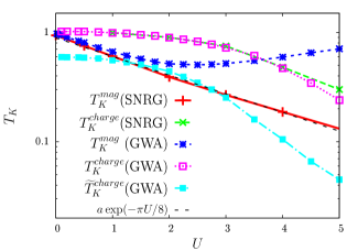
Figure 2: The equilibrium low-energy scales as functions of $U$ extracted from the various approximations as described in the text. A fit to the magnetic scale of the NRG to show the exponential decay $\propto\exp(-\pi U/8)$ is also included in the plot.

Figure 2 shows the two scales extracted from NRG and GWA calculations for a symmetric junction in equilibrium. The NRG results show the expected $U$-dependencies: The charge scale $T_{K}^{charge}$ is on the order of $\Gamma$ for small $U\apprle 3\Gamma$ and decreases exponentially for large $U\apprge 4\Gamma$. The magnetic scale $T_{K}^{mag}$ decreases exponentially for all $U$ as it is evident from the comparison with a fit function $a\exp(-\pi U/8)$ also included in the plot. Furthermore, there exists only one universality scale for large $U$ which manifests itself by $T_{K}^{mag}\propto T_{K}^{charge}$ (not shown).

On the other hand, the scales obtained from the GWA agree with the NRG only for small $U$. The charge scale $T_{K}^{charge}$ perfectly agrees with the NRG curve for $U\apprle 4$. Significant deviations are observed for larger $U$, where the GWA-$T_{K}^{charge}$ decreases faster than the NRG. For $U$ significantly larger than the ones shown in the plot, no scales could be extracted due to the artificial symmetry breaking already reported in the literature.Wang et al. (2008); Thygesen and Rubio (2008)

We added a second GWA charge scale $\widetilde{T}_{K}^{charge}$ to the graph which is obtained from the width of the low-energy feature at $75\%$ of $\rho^{r}(0)$ (and not at the FWHM as for $T_{K}^{charge}$). The correspondingly extracted scale should coincide with $T_{K}^{charge}$, apart from a prefactor. But it is found that both scales follow the same trend only for small $U$ and already for $U\apprge 3$ a much stronger decrease than the expected $\exp(-\pi U/8\Gamma)$ is observed in $\widetilde{T}_{K}^{charge}$ .

Figure 3: Comparison of the NRG and the Keldysh GWA equilibrium ($V=0$) zero-temperature spectral functions for $U/\Gamma=4$ and $E_{d}=-U/2$ and a quantum-point contact $\Gamma_{L}=\Gamma_{R}=1/2$. The inset shows the temperature evolution of the spectral function right at the Fermi level, $\rho^{r}(\omega=0,T)$. The NRG-parameters are $\Lambda=2$, $N_{s}=1500$, $N_{z}=4$, $b=0.325$ and $50$ NRG iterations were performed.

Therfore, the extraction of the charge scale within the GWA at intermediate $U$ is somewhat ambiguous. A comparison of the zero-temperature equilibrium spectral function of the GWA and NRG for $U=4\Gamma$ is depicted in Fig. 3. The low-energy feature of the GWA spectral function is too narrow and exhibits a rather spiky line-shape which suggest at too low charge scale. This is supported by the evolution of $\rho^{r}(0)$ as a function of temperature which is shown in the inset of Fig. 3. The logarithmic increase of $\rho^{r}(0)$ which occurs at temperatures on the order of the relevant charge scale also reveals that the charge scale is predicted as too low in GWA compared to the NRG. However, a considerable broadening occurs away from the Fermi level which leads to the same FWHM for the GWA as in the NRG and consequently the larger $T_{K}^{charge}$ emerges in thermodynamic quantities like $G(T)$.

The magnetic scale $T_{K}^{mag}$ extracted from the GWA exhibits some peculiar $U$-dependence. For small $U\apprle\Gamma$ the scale agrees with the NRG. However, it develops a minimum at $U\approx 2.5\Gamma$ and then increases again for increasing $U$! This clearly indicates a failure of the GWA to describe magnetic properties for intermediate and large interactions. Since the GWA effective moments $\mu_{eff}^{2}$ show universality as functions of the dimensionless temperature $t=T/T^{mag}_{K}$ for low temperatures (not shown), the increase in $T_{K}^{mag}$ implies a too strong screening of magnetic moments. The effective Coulomb interaction is over-screened by $W$ (see Eq. (33)). The electrons remain itinerant even at rather large $U$, and the GWA fails to capture the atomic limit. Therefore, the magnetic screening scale $T_{K}^{mag}$ remains large in the GWA and actually increases with $U$.

The scales extracted from the other two diagrammatic approximations all coincide with the GWA for small $U\apprle\Gamma$. For larger $U$ the $2^{nd}U$ approximation produces the same difference as the GWA between the charge and the magnetic scale, whereas within the 2BA both scales decrease with increasing $U$, but in a polynomial rather than exponential fashion.

We have established that the diagrammatic approach produces reliable results for interactions up to the order of the hybridization strength $U\apprle\Gamma$ which we will use in the following section to benchmark the SNRG in that regime.

III.2 Weak correlation regime: $U\apprle\Gamma$

We study the nonequilibrium properties of a symmetric and an asymmetric junction in the weakly correlated regime $U/\Gamma\apprle 1$. We use a very low temperature $T=0.006\Gamma$, which is sufficiently small compared to all other scales in the problem so it can be considered as $T=0$ with impunity.

For such small interactions the diagrammatic approaches and the SNRG yield identical results for all voltages. Figure 4(a) shows the nonequilibrium spectral function of a symmetric junction in the quantum-point contact regime, i.e. $U=-2E_{d}=\Gamma=1$ and $\Gamma_{L}=\Gamma_{R}=\Gamma/2=0.5$. For small voltages $V/\Gamma\apprle 0.5$ the spectra are even indistinguishable from the Hartree-Fock (HF) result. Only at larger $V$ small deviations around the Fermi level as can be observed.

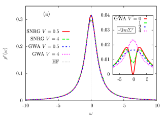
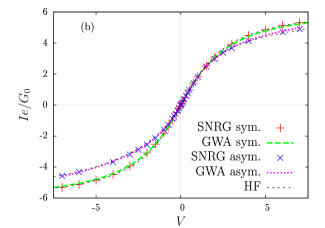
Figure 4: (a) Spectral function of the retarded Green’s function and negative imaginary part of the retarded self-energy (inset) of a symmetric junction with $U=-2E_{d}=1$ and $\Gamma_{L}=\Gamma_{R}=0.5$ for different voltages. Results for the spectral functions are shown for HF, GWA and SNRG, while the self-energy is shown for the GWA only. (b) Current as a function of voltage for a symmetric ($U=-2E_{d}=1$ and $\Gamma_{L}=\Gamma_{R}=0.5$) and an asymmetric junction ( $U=1$, $E_{d}=-0.25$ and $\Gamma_{L}=4\Gamma_{R}=0.8$). $I$ is normalized to $G_{0}/e=h/e$ (symmetric) and $G_{0}/e=0.64h/e$ (asymmetric) and measured in units of $\Gamma=1$. A small temperature of $T=0.006$ was used for all calculations. Parameters for the SNRG calculations are $\Lambda=4$, $N_{s}=2200$, $N_{z}=2$, $b=0.65$ and 12 NRG-iterations were performed.

The imaginary part of the retarded self-energy $-\Im m[\Sigma^{r}(\omega)]$ for that junction obtained with the GWA is shown in the inset of Fig. 4(a) for various voltages. The overall scale of $-\Im m[\Sigma^{r}(\omega)]$ is much smaller than $\Gamma$ and, therefore, the total self-energy $\Sigma^{tot}=\Sigma^{r}+\Delta$ is dominated by the charge-fluctuation scale $\Gamma$. But the general influence of a finite bias voltage can already be observed here: The quasiparticle scattering amplitude is increased by the interplay between the voltage-induced fluctuations and the interaction. The characteristic Fermi-liquid quadratic minimum in $-\Im m[\Sigma^{r}(\omega)]$ at the Fermi level is destroyed with increasing voltage and the local Fermi liquid prevailing in equilibrium ($V=0$) is suppressed at large enough bias. The evolution of the minimum in $-\Im m[\Sigma^{r}(\omega)]$ with voltage bears some resemblance with a temperature evolution. The quasi-particle coherence is destroyed by a finite voltage in a similar fashion as with increasing temperature.

The resulting IV characteristics of a symmetric and an asymmetric junction are shown in Fig. 4(b) for $U=\Gamma$. The current is normalized to $G_{0}/e$ and measured in units of $\Gamma$. The rescaled current always saturates at $2\pi\Gamma$ for large voltages independent of $U$ (not shown), as required by Eq. (43). The initial slope at zero voltage of the IV curve remains unaltered for all values of $U$, in accordance with the Fermi liquid nature of the model at small bias and zero temperature.

While a symmetric junction with symmetric coupling to the leads always results in symmetric spectral functions, $\rho^{r}(\omega,V)=\rho^{r}(\omega,-V)$, and antisymmetric IV characteristics, $I(-V)=-I(V)$ (see Eq. (43)), an asymmetric junction in combination with asymmetric coupling yields a non-antisymmetric IV characteristics with $I(-V)\neq-I(V)$. This is clearly visible in Fig. 4(b). The bias window ranges from $\mu_{L}=-r_{R}^{2}V$ to $\mu_{R}=r_{L}^{2}V$ and is not symmetric around the Fermi level. In combination with the shift of spectral weight to higher energies in $\rho^{r}(\omega)$ — the center of the spectral function is at $2E_{d}+U>0$ — this leads to a smaller contribution to the current for negative voltages.

In contrast to the spectral functions, the IV characteristics of the SNRG and GWA agree perfectly with the HF results for all voltages. The current is rather insensitive to the detailed distribution of spectral weight and measures only the total amount in the bias window $[\mu_{L},\mu_{R}]$.

The SNRG produces the correct results for small values of the interaction $U\apprle\Gamma$, and has thus no principal limitations. Therefore, the expectation that it is reliable at arbitrary interaction strengths as well is warranted.

III.3 Intermediate correlation regime: $\Gamma\apprle U\apprle 10\Gamma$

As demonstrated in the previous section the interaction plays a minor role for small $U/\Gamma$. On the other hand, with an odd number of electrons on the quantum dot and at very large $U/\Gamma$ and $\Gamma-U\ll E_{d}\ll-\Gamma$, the system develops a Kondo effect as $T\to 0$ (see for example Ref. Hewson, 1993a and kon, 2005). The SNRG was shown Anders (2008a) to correctly describe the strongly correlated Kondo regime out of equilibrium. The enhancement of the conductance in the Coulomb-blockade region was reproduced for small bias, and the destruction of the many-body resonance at the Fermi level with increasing voltage has been studied.

In this section we will focus on the intermediate interaction regime, where correlations become increasingly important. Since the diagrammatic Keldysh approximations already show deficiencies in equilibrium — see, for example, in Sec. III.1 or Ref. Wang et al., 2008 — discrepancies will extend to finite voltages.

III.3.1 Nonequilibrium spectral functions of a symmetric junction

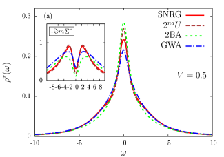
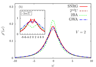
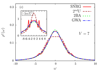
Figure 5: Spectral functions of the SNRG and the Keldysh approaches for a quantum-point contact with $\Gamma_{L}=\Gamma_{R}=0.5$ and $U=-2E_{d}=4$ at $T=0.1$. The bias voltages are $V=0.5$ (a), $V=2$ (b) and $V=7$ (c). SNRG-parameters are $\Lambda=4$, $N_{s}=2200$, $N_{z}=4$, $b=0.325$ and 8 NRG-iterations were performed.

The nonequilibrium spectral function for various voltages and intermediate interaction $U=4$ is shown in Fig. 5(a)-(c) for a symmetric junction ($E_{d}=-2$) with symmetric coupling to the leads ($\Gamma_{L}=\Gamma_{R}=\Gamma/2=0.5$) at $T=0.1$. Now all diagrammatic approximations yield different results.

At low voltages, the SNRG and $2^{nd}U$ approximation reproduce the slight humps at energies $\omega\approx\pm U/2$ which are the first indicators of upper and lower Hubbard satellites forming at large $U$. The GWA only produces the broad high-energy tails, without the indication of forming separate peaks and the 2BA completely fails to produce the enlarged spectral weight at high energies.

As the voltage is raised, the Coulomb interaction causes additional dephasing, leading to increasingly broadened spectra. However, the $2^{nd}U$ approximation produces systematically too broad high-energy tails and an unphysical plateau around $\omega=0$, which even develops a slight dip as seen in Fig. 5(c). We attribute this to a tendency to overestimate the Coulomb repulsion. This might already be guessed from the equilibrium spectral functions, where the $2^{nd}U$ approximation unexpectedly produces the high-energy Hubbard satellites for arbitrary large Coulomb repulsion. These are connected to the ionic many-body states of the isolated atom which are not expected to be described by a second-order perturbation theory. However, the analytic structure of the retarded self-energy, Eq. (30), (32), (36) and (39), has two direct consequences: (i) For small coupling to the leads or large $U$ it favors a $\Sigma^{r}(\omega)\propto U^{2}/(\omega+i\delta)$ behavior. This results in a two-peak structure with the peak-positions and widths roughly given by $\pm U$ and $\Gamma$, respectively. (Incorporating a screened and dynamic Coulomb interaction, as it is done in the 2BA and GWA, leads to a prefactor smaller than $U^{2}$ and additional imaginary parts enter in the frequency dependence of $\Sigma^{r}(\omega)$. The Hubbard satellites are then moved to lower energies and broadened.) (ii) The Fermi functions entering Eq. (36) through $G^{<}$ lead to a narrowing of the integration interval for decreasing temperature. At zero temperature this always produces a vanishing imaginary part of the self-energy at the Fermi level, $\Im m[\Sigma^{r}(\omega=0,T=0)]=0$,Luttinger (1961) given that the noninteracting propagators are non-singular at $\omega=0$. (This reasoning also holds for the 2BA and GWA).

The combination of (i) and (ii) gives rise to the two-peak structure in the spectral function for large $U$ and the emergence of an additional peak at the Fermi level for low temperatures which is usually interpreted as the Kondo resonance. But in principle there is no justification why the $2^{nd}U$ approximation should be reliable for large values of $U$ under arbitrary conditions. Already for the asymmetric model in equilibrium the phase-space argument (ii) does not guarantee the correct description of the low-temperature Fermi liquid anymore, and it is well-known that the $2^{nd}U$ approximation produces unphysical results.Ferrer et al. (1987); Kajueter and Kotliar (1996) Therefore, the large differences to all other methods at finite voltages, as it is observed here for $U/\Gamma=4$, is not surprising.

The SNRG tends to produce additional features in the spectral function for large bias voltages at the positions of the chemical potentials of the leads, $\omega\approx\mu_{\alpha}$. These are the humps visible for larger voltages in the curves of Fig. 5. They are artifacts of the NRG discretization and dependent on the broadening procedure of the NRG spectral functions.Bulla et al. (2008a) In equilibrium, the NRG only resolves spectral information above a cutoff frequency $|\omega|>\omega_{c}(T)$ where $\omega_{c}$ is on the order of the temperature $T$. The NRG broadening parameters Costi et al. (1994); Bulla et al. (2001); Peters et al. (2006); Bulla et al. (2008a) are usually adjusted such that artefacts are minimized. Additionally the spectral function is interpolated between $-\omega_{c}<\omega<\omega_{c}$. This translates itself to the present implementation of the SNRG which does not provide spectral information in the intervals $I^{\pm}=[\mu^{\pm}-\omega_{c}:\mu^{\pm}+\omega_{c}]$ centered around the two chemical potentials. Here, $\mu^{+}=\mbox{max}\{\mu_{L},\mu_{R}\}$ and $\mu^{-}=\mbox{min}\{\mu_{L},\mu_{R}\}$. Furthermore, the time-dependent NRG introduces additional discretization errorsAnders and Schiller (2006) which increase with increasing value of $U$. $z$-averaging over different discretizationsYoshida et al. (1990) improves the spectral functions and these artifacts could be removed by adjusting the broadening parameter depending on the voltage. In this paper, however, we keep the broadeningCosti et al. (1994); Bulla et al. (2001); Peters et al. (2006); Bulla et al. (2008a) parameter fixed at $b=1.3/N_{z}$ independent of the bias and performed $z$-averaging with $N_{z}=2$ and $4$.

Let us focus on the different behavior of the spectral functions around $\omega=0$ depicted in Fig. 5(a)-(c). The height $\rho^{r}(0)$ is reduced for increasing $V$, and the spectral functions of the SNRG, 2BA and GWA approach each other and eventually coincide. For $V=7$, the 2BA curve is still a little higher compared to SNRG and GWA, but at even larger voltages (not shown) it also falls on top of the SNRG and GWA. In contrast, the $2^{nd}U$ spectral function does not approach this large voltage limit, and the zero frequency value of the spectral function is considerably reduced compared to the other approaches. This is in accord with an enhanced scattering amplitude at the Fermi level, visible in the imaginary part of the self-energy depicted in the insets.

Upon increasing the voltage, the $2^{nd}U$ approximation does not follow a systematic trend since $\rho^{r}(0)$ is larger than the SNRG at low voltages and smaller at high $V$. The other approximations show systematic deviations as the 2BA is always larger than the SNRG, while the GWA is always smaller.

In the present calculations, the temperature $T=0.1$ is only about on fifth of the equilibrium Kondo temperature for these parameter values, i.e. $T/T_{K}\approx 0.2$. As discussed in Sec. III.1, the GWA produces a too small charge scale, which results in an even higher effective temperature. This leads to a reduction of the spectral function at the Fermi level in addition to the effect of the small bias. The imaginary part of the self-energy is correspondingly too large compared to the SNRG, as can be seen in the inset of Fig. 5(a). The 2BA, on the other hand, overestimates the low-energy scale, which explains the trends in $\rho^{r}(0)$ and $-\Im m[\Sigma^{r}(0)]$.

Increasing the current through the junction by applying a larger bias enhances the charge fluctuations on the local orbital. As already mentioned in section III.2, theses additional fluctuations introduce dephasingKehrein (2005) and destroy the coherent quasiparticles which constitute the low-temperature Fermi liquid. The accompanying destruction of the characteristic quadratic minimum in $-\Im m[\Sigma^{r}(\omega)]$ around $\omega\approx 0$ is observed in the insets. The system is driven away from the equilibrium Fermi-liquid fixed point, and the spectral functions at the Fermi level decreases. At very large voltage $|V/T_{K}|\gg 1$ the coherent quasiparticles are completely suppressed, as it can be seen from the large imaginary part of the self-energy around $\omega\approx 0$. The spiky features in the SNRG self-energy for $V=7$ are due to the aforementioned discretization errors and have no physical meaning.

III.3.2 IV characteristics of a symmetric junction

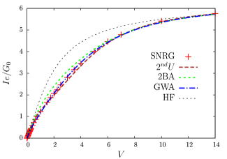
Figure 6: IV characteristics for $U=-2E_{d}=4$ obtained from the spectral functions presented in Fig. 5 for a quantum-point contact with $\Gamma_{L}=\Gamma_{R}=0.5$. The current is normalized to $G_{0}/e=h/e$ and measured in units of $\Gamma=1$.

A Coulomb interaction $U/\Gamma=4$ leads to a reduction of the current compared to its HF value as depicted in Fig. 6. This is characteristic for the onset of the Coulomb blockade. All approaches predict this reduction but slight differences can be noticed. The $2^{nd}U$ approximation overestimates the Coulomb blockade resulting in a current which is systematically smaller than the SNRG result. Even though the $2^{nd}U$ spectral function differs strongly from all other approaches for large $V$, this failure to describe the correct single-particle dynamics is concealed in the current as all approaches yield identical results. It again shows the insensitivity of the current to the detailed distribution of spectral weight in $\rho^{r}(\omega)$. The 2BA slightly overestimates the current for intermediate voltages, which is again explained by the too large low-energy scale $T_{K}^{charge}$ and the accompanying underestimation of correlation effects.

The GWA current merges with the SNRG result for $V\apprge 2$, which — together with the satisfactory spectral function for these voltages — indicates a good description of the nonequilibrium properties for intermediate to large $V$.

III.3.3 Asymmetric junction

The spectral function for a quantum dot with a level position $E_{d}=-1$, Coulomb interaction $U=4$ and asymmetric coupling $\Gamma_{L}=4\Gamma_{R}=0.8$ is shown in Fig. 7. The asymmetry between positive and negative voltages is directly visible in the spectral functions.

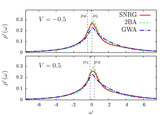
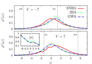
Figure 7: Spectral functions for the asymmetric junction, $U=4$, $E_{d}=-1$, with asymmetric coupling $\Gamma_{L}=4\Gamma_{R}=0.8$ for small (upper) and large (lower) bias, $V=\pm 0.5$ and $V=\pm 7$, respectively. The vertical dashed lines indicate the location of the left and right chemical potentials. The inset shows the total occupation $\langle\hat{n}\rangle$ of the impurity as a function of the bias voltage obtained with the diagrammatic approaches. SNRG-parameters are the same as for Fig. 5.

Apart from voltage-induced broadening which was already discussed in previous sections, an additional shift of spectral weight in $\rho^{r}(\omega)$ is observed with increasing $V$. While the SNRG moves spectral weight to higher energies for positive bias and towards $\omega=0$ for negative $V$, the diagrammatic approaches produce the opposite trends.

Due to the stronger coupling to the left lead, $\Gamma_{L}=4\Gamma_{R}$, the left-moving scattering states dominate the excitations and the spectral function of the impurity orbital, as can be seen from Eq. (9) and (10). The effective noninteracting single-particle excitation energy of an $\alpha$-mover is given by $\Delta\epsilon_{\alpha}=E_{d}-\mu_{\alpha}$, which implies almost symmetric parameters for the left-movers at the negative voltage $V=-7$ since then $\Delta\epsilon_{L}=-2.4$. Therefore, the asymmetry of the spectral function is expected to be reduced and $\rho^{r}(\omega)$ to be closer to that of a symmetric junction, which is indeed observed in the SNRG.

The diagrammatic approaches underestimate correlations in the ionic many-body states, and the occupancy of the impurity is overestimated for negative voltages. It increases almost linearly with negative voltage as can be seen from the inset of Fig. 7(b). Therefore, the Hartree shift (28) also increases, and spectral weight is moved towards higher energies opposite to what would be expected from the physical argument presented above. As a consequence the spectral functions are strongly attracted to $\mu_{L}$.

The effective single-particle excitation energy of a left-moving scattering state for a positive voltage $V=7$ is greater than zero, $\Delta\epsilon_{L}=0.4$. This produces an intermediate valence situation for the left-movers, where correlations renormalize the effective excitation energies to even larger frequenciesKrishna-murthy et al. (1980b) and a shift of spectral weight to higher energies results. An additional drag of spectral weight towards the chemical potential of the weaker coupled right lead, $\mu_{R}=0.8V=5.6$, is expected. The SNRG produces such a shift as can be seen in Fig. 7(b). The diagrammatic approaches, however, underestimate the level-renormalization in the presence of strong valence fluctuations, a tendency already observable in equilibrium (not shown). Additionally, the reduced occupancy (inset) diminishes the Hartree energy which again leads to a shift towards the stronger coupled chemical potential $\mu_{L}=-1.4$.

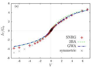
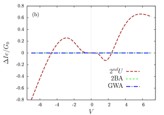
Figure 8: (a) IV characteristics of the asymmetric junction, $E_{d}=-1$, $U=4$ and $\Gamma_{L}=4\Gamma_{R}=0.8$, calculated with the spectral functions depicted in Fig. 7. The result for the symmetric junction already shown in Fig. 6 is included for comparison. (b) The leakage current $\Delta I(V)$ for the Keldysh approaches obtained from Eq. (II.4). The currents are normalized to $G_{0}/e=0.64h/e$ and measured in units of $\Gamma=1$.

Figure 8 shows the IV characteristics of this junction. The asymmetry of $I(V)$ is clearly visible when compared to the result from the symmetric junction (also included in the plot). For $V>0$, the rescaled current is very close to its values from the symmetric junction and the discrepancies between the 2BA, GWA and SNRG follow the already discussed characteristics: The 2BA underestimates correlations and yields a slightly too large current. The GWA has the correct distribution of spectral weight in the bias window and produces a rather good estimate for the current, despite its deficiencies in the description of the single-particle spectra. The failure to produce the correct shifts of spectral weights in $\rho^{r}(\omega)$ causes the current in the diagrammatic approaches to be smaller than the SNRG for negative voltages.

The $2^{nd}U$ approximation, however, reveals its non-conserving nature in the violation of current conservation for this asymmetric junction. This is illustrated in Fig. 8(b) displaying the leakage current $\Delta I$ of Eq. (II.4). In contrast to the conserving 2BA and GWA methods and the SNRG, $\Delta I$ does not vanish for the $2^{nd}U$ approximation! Thus, left and right current of Eq. (42) do not have the same magnitude, i.e. $I_{L}\neq-I_{R}$, and the current calculated from Eq. (43) does not make sense, since different linear combinations $aI_{L}-(1-a)I_{R}$ ($0\leq a\leq 1$) yield different results. Therefore, we did not include the calculated IV curves in Fig. 8(a).

Increasing the asymmetry further, i.e. $\Gamma_{L}\gg\Gamma_{R}$, recovers the equilibrium spectral functions of a quantum dot coupled to a single lead in all approaches (not shown). In the SNRG, the backscattering term $\hat{O}_{\sigma}^{back}$, Eq. (13), is suppressed, and the model approaches an equilibrium single-channel problem. In the diagrammatic approaches, the nonequilibrium conditions enter only through the effective Fermi function $f_{\mbox{eff}}$, Eq. (27), which approaches its equilibrium value for $\Gamma_{R}\to 0$. In this regime, all differences in the spectral functions of the presented approaches are given by the known discrepancies already present in equilibrium.

IV Summary

In the recently developed SNRG approach to open quantum systems the scattering states of a noninteracting quantum impurity model are used to construct the nonequilibrium Green’s functions for the steady state at finite bias voltage. We have established the reliability of the SNRG by benchmarking it against the diagrammatic Kadanoff-Baym-Keldysh approach, which becomes exact in the limit $U\to 0$. It has been shown that the spectra and the current-voltage characteristics agree excellently for small Coulomb interactions for symmetric and asymmetric junctions at arbitrary bias voltage.

For intermediate values of $U$ we have compared the SNRG to three different approximations obtained from the Keldysh approach, namely the second-order perturbation theory ($2^{nd}U$), the fully self-consistent second-order (2BA) and the GW approximation (GWA). As correlation effects play an increasingly important role discrepancies occur between the different methods. These were explained by the insufficient treatment of the Coulomb interaction within the diagrammatic approaches.

The Fermi liquid at zero bias voltages is characterized by a single low-energy scale which is captured accurately by the SNRG, but is not properly reproduced by the diagrammatic approaches. No single low-energy scale can be extracted from the $2^{nd}U$ approximation and the GWA at intermediate and large $U$. While the scale associated with charge fluctuations decreases with increasing $U$, the magnetic scale exhibits a qualitatively different $U$-dependency, since it develops a minimum for intermediate $U$ and increases again towards larger $U$! The GWA shows a tendency to over-screen magnetic moments for increasing values of $U$ and fails to reproduce the atomic limit. These deficiencies translate themselves to finite bias and explain the discrepancies at small to intermediate voltages.

At large bias voltages the self-consistent diagrammatic approaches (2BA and GWA) reproduce the SNRG spectral functions for a symmetric junction, while the second-order perturbation theory yields an unphysical plateau around the Fermi level.

All diagrammatic approximations and the SNRG capture the onset of the Coulomb blockade in the IV characteristics of the symmetric junction. The small discrepancies are explained by the deficiencies in the treatment of the interaction. However, the failure of the $2^{nd}U$ approximation to correctly describe the single-particle dynamics at large bias is masked in the current, since there only the total spectral weight in the bias window enters.

In contrast to the other methods, the $2^{nd}U$ approximation reveals its non-conserving nature by producing a finite leakage current for an asymmetric junction, which is unphysical. This raises the question about the reliability of the results obtained within that method or extensions of it,Yeyati et al. (1993); Takagi and Saso (1999); Fujii and Ueda (2003, 2005); Aligia (2006) even for a symmetric junction. They are only well-justified for cases where $|\Sigma^{r}(\omega)|\ll\Gamma$ for all frequencies.

The voltage dependent redistribution of spectral weight for an asymmetric junction is not well-reproduced by the diagrammatic approaches. This has been attributed to too large Hartree shifts due to the wrong occupation number of the impurity and the inaccurate renormalization of the single-particle level in intermediate-valence situations. It leads to the underestimation of the current for large negative voltages.

The SNRG provides access to the description of nonequilibrium steady-state properties of nanoscale junctions for arbitrary Coulomb interaction and voltages. It opens promising perspectives for future investigations, such as the influence of charge fluctuations when approaching the strongly-correlated regime or the effects of an applied magnetic field.

V Acknowledgments

We are grateful to J. E. Han, A. Millis, A. Schiller, P. Schmitteckert, G. Schön, H. Schoeller, P. Werner, M. Wegewijs and G. Zarand for helpful discussions. We acknowledge financial support from the Deutsche Forschungsgemeinschaft under AN 275/6-1 and supercomputer support by the NIC, Forschungszentrum Jülich under project No. HHB000.

References

- Elzerman et al. (2004) J. M. Elzerman, R. Hanson, L. H. W. van Beveeren, B. Witkamp, L. M. K. Vandersypen, and L. P. Kouvenhoven, Nature 430, 431 (2004).
- Nitzan and Ratner (2003) A. Nitzan and M. A. Ratner, Science 300, 1384 (2003).
- Temirov et al. (2008) R. Temirov, A. Lassise, F. B. Anders, and F. S. Tautz, Nanotechnology 19, 065401 (2008).
- Goldhaber-Gordon et al. (1998a) D. Goldhaber-Gordon, H. Shtrikman, D. Mahalu, D. Abusch-Magder, U. Meirav, and M. Kastner, Nature 391, 156 (1998a).
- Goldhaber-Gordon et al. (1998b) D. Goldhaber-Gordon, J. Göres, M. A. Kastner, H. Shtrikman, D. Mahalu, and U. Meirav, Phys. Rev. Lett. 81, 5225 (1998b).
- van der Wiel et al. (2000) W. G. van der Wiel, S. D. Franceschi, T. Fujisawa, J. M. Elzerman, S. Tarucha, and L. P. Kouwenhoven, Science 289, 2105 (2000).
- Nagaoka et al. (2002) K. Nagaoka, T. Jamneala, M. Grobis, and M. F. Crommie, Phys. Rev. Lett. 88, 077205 (2002).
- Quay et al. (2007) C. H. L. Quay, J. Cumings, S. J. Gamble, R. de Picciotto, H. Kataura, and D. Goldhaber-Gordon, Phys. Rev. B 76, 245311 (2007).
- Grobis et al. (2008) M. Grobis, I. G. Rau, R. M. Potok, H. Shtrikman, and D. Goldhaber-Gordon, Phys. Rev. Lett. 100, 246601 (2008).
- Amasha et al. (2005) S. Amasha, I. J. Gelfand, M. A. Kastner, and A. Kogan, Phys. Rev. B 72, 045308 (2005).
- Liu et al. (2009) T.-M. Liu, B. Hemingway, A. Kogan, S. Herbert, and M. Melloch, Phys. Rev. Lett. 103, 026803 (2009).
- Hewson (1993a) A. C. Hewson, The Kondo Problem to Heavy Fermions (Cambridge University Press, Cambridge, 1993a).
- kon (2005) Special Topic Series: Kondo Effect - 40 Years after the Discovery, vol. 74 of J. Phys. Soc. Jpn. (2005).
- Anders (2008a) F. B. Anders, Phys. Rev. Lett. 101, 066804 (2008a).
- Wingreen and Meir (1994) N. S. Wingreen and Y. Meir, Phys. Rev. B 49, 11040 (1994).
- Anders (2008b) F. B. Anders, J. Phys.: Condens. Matter 20, 195216 (2008b).
- Thygesen and Rubio (2007) K. S. Thygesen and A. Rubio, J. Chem. Phys. 126, 091101 (2007).
- Darancet et al. (2007) P. Darancet, A. Ferretti, D. Mayou, and V. Olevano, Phys. Rev. B 75, 075102 (2007).
- Spataru et al. (2009) C. D. Spataru, M. S. Hybertsen, S. G. Louie, and A. J. Millis, Phys. Rev. B 79, 155110 (2009).
- Myohanen et al. (2009) P. Myohanen, A. Stan, G. Stefanucci, and R. van Leeuwen, arXiv:0906.2136 (2009).
- Keldysh (1965) L. V. Keldysh, Sov. Phys. JETP 20, 1018 (1965).
- Yeyati et al. (1993) A. L. Yeyati, A. Martín-Rodero, and F. Flores, Phys. Rev. Lett. 71, 2991 (1993).
- Takagi and Saso (1999) O. Takagi and T. Saso, J. Phys. Soc. Jpn. 68, 1997 (1999).
- Matsumoto (2000) D. Matsumoto, J. Phys. Soc. Jpn. 69, 1449 (2000).
- Fujii and Ueda (2003) T. Fujii and K. Ueda, Phys. Rev. B 68, 155310 (2003).
- Bulla et al. (2008a) R. Bulla, T. A. Costi, and T. Pruschke, Rev. Mod. Phys. 80, 395 (2008a).
- Andrei et al. (1983) N. Andrei, K. Furuya, and J. H. Lowenstein, Rev. Mod. Phys. 55, 331 (1983).
- Tsvelick and Wiegmann (1983) A. M. Tsvelick and P. B. Wiegmann, Adv. Phys. 32, 453 (1983).
- Affleck and Ludwig (1991) I. Affleck and A. W. W. Ludwig, Nucl. Phys. B 360, 641 (1991).
- Affleck and Ludwig (1993) I. Affleck and A. W. W. Ludwig, Phys. Rev. B 48, 7297 (1993).
- Wilson (1975) K. G. Wilson, Rev. Mod. Phys. 47, 773 (1975).
- Kaminski et al. (2000) A. Kaminski, Y. V. Nazarov, and L. I. Glazman, Phys. Rev. B 62, 8154 (2000).
- Rosch et al. (2001) A. Rosch, J. Kroha, and P. Wölfle, Phys. Rev. Lett. 87, 156802 (2001).
- Jakobs et al. (2007) S. G. Jakobs, V. Meden, and H. Schoeller, Phys. Rev. Lett. 99, 150603 (2007).
- Gezzi et al. (2007) R. Gezzi, T. Pruschke, and V. Meden, Phys. Rev. B 75, 045324 (2007).
- Doyon and Andrei (2006) B. Doyon and N. Andrei, Phys. Rev. B 73, 245326 (2006).
- Mehta and Andrei (2006) P. Mehta and N. Andrei, Phys. Rev. Lett. 96, 216802 (2006).
- Kehrein (2005) S. Kehrein, Phys. Rev. Lett. 95, 056602 (2005).
- Kehrein (2006) S. Kehrein, The Flow Equation Approach to Many-Particle Systems, vol. 217 of Springer Tracts in Modern Physics (Springer, Heidelberg, 2006).
- Schoeller and Koenig (2000) H. Schoeller and J. Koenig, Phys. Rev. Lett. 84, 3686 (2000).
- Schoeller (2009) H. Schoeller, Eur. Phys. J. Special Topics 168, 179 (2009).
- Pletyukhov et al. (2009) M. Pletyukhov, D. Schuricht, and H. Schoeller, arXiv:0910.0119 (2009).
- Hershfield (1993) S. Hershfield, Phys. Rev. Lett. 70, 2134 (1993).
- Schmitteckert (2004) P. Schmitteckert, Phys. Rev. B 70, 121302(R) (2004).
- Schollwöck (2005) U. Schollwöck, Rev. Mod. Phys. 77, 259 (2005).
- Kirino et al. (2008) S. Kirino, T. Fujii, J. Zhao, and K. Ueda, J. Phys. Soc. Jpn. 77, 084704 (2008).
- Heidrich-Meisner et al. (2009) F. Heidrich-Meisner, A. E. Feiguin, and E. Dagotto, Phys. Rev. B 79, 235336 (2009).
- Boulat et al. (2008) E. Boulat, H. Saleur, and P. Schmitteckert, Phys. Rev. Lett. 101, 140601 (2008).
- Han and Heary (2007) J. E. Han and R. J. Heary, Phys. Rev. Lett. 99, 236808 (2007).
- Dirks et al (2010) A. Dirks, P. Werner, M. Jarrell and Th. Pruschke, arXiv:1002.4081 (2010).
- Mühlbacher and Rabani (2008) L. Mühlbacher and E. Rabani, Phys. Rev. Lett. 100, 176403 (2008).
- Werner et al. (2009) P. Werner, T. Oka, and A. J. Millis, Phys. Rev. B 79, 035320 (2009).
- Werner et al. (2010) P. Werner, T. Oka, M. Ekstein, and A. J. Millis, Phys. Rev. B 81, 035108 (2010).
- Weiss et al. (2008) S. Weiss, J. Eckel, M. Thorwart, and R. Egger, Phys. Rev. B 77, 195316 (2008).
- Schweber (1962) S. S. Schweber, Relativistic quantum field theory (Harper & Row, New York, 1962).
- Han (2006) J. E. Han, Phys. Rev. B 73, 125319 (2006).
- Schiller and Hershfield (1995) A. Schiller and S. Hershfield, Phys. Rev. B 51, 12896 (1995).
- Schiller and Hershfield (1996) A. Schiller and S. Hershfield, Phys. Rev. Lett. 77, 1821 (1996).
- Schiller and Hershfield (2000) A. Schiller and S. Hershfield, Phys. Rev. B 62, R16271 (2000).
- Oguri (2007) A. Oguri, Phys. Rev. B 75, 035302 (2007).
- Anders and Schiller (2005) F. B. Anders and A. Schiller, Phys. Rev. Lett. 95, 196801 (2005).
- Anders and Schiller (2006) F. B. Anders and A. Schiller, Phys. Rev. B 74, 245113 (2006).
- Enss et al. (2005) T. Enss, V. Meden, S. Andergassen, X. Barnabe-Theriault, W. Metzner, and K. Schoenhammer, Phys. Rev. B 71, 155401 (2005).
- Lebanon et al. (2003) E. Lebanon, A. Schiller, and F. B. Anders, Phys. Rev. B 68, 041311(R) (2003).
- Hershfield et al. (1991a) S. Hershfield, J. H. Davies, and J. W. Wilkins, Phys. Rev. Lett. 67, 003720 (1991a).
- Meir and Wingreen (1992a) Y. Meir and N. S. Wingreen, Phys. Rev. Lett. 68, 2512 (1992a).
- Yoshida et al. (1990) M. Yoshida, M. A. Whitaker, and L. N. Oliveira, Phys. Rev. B 41, 9403 (1990).
- Peters et al. (2006) R. Peters, T. Pruschke, and F. B. Anders, Phys. Rev. B 74, 245114 (2006).
- Kadanoff and Baym (1962) L. P. Kadanoff and G. Baym, Quantum Statistical Mechanics (Benjamin, 1962).
- Danielewicz (1984) P. Danielewicz, Ann. Phys. 152, 239 (1984).
- Wagner (1991) M. Wagner, Phys. Rev. B 44, 6104 (1991).
- van Leeuwen et al. (2006) R. van Leeuwen, N. E. Dahlen, G. Stefanucci, C.-O. Almbladh, and U. von Barth, Lect. Notes Phys. 706, 33 (2006).
- Haug and Jauho (1996) H. Haug and A.-P. Jauho, Quantum Kinetics in Transport and Optics of Semiconductors (Springer, Berlin, 1996).
- Luttinger and Ward (1960) J. M. Luttinger and J. C. Ward, Phys. Rev. 118, 1417 (1960).
- Yamada (1975) K. Yamada, Prog. Theor. Phys. 54, 316 (1975).
- Horvatic and Zlatic (1980) B. Horvatic and V. Zlatic, Phys. Status Solidi (b) 99, 251 (1980).
- Chen and Bickers (1992) C.-X. Chen and N. E. Bickers, Solid State Commun. 82, 311 (1992).
- White (1992) J. A. White, Phys. Rev. B 45, 1100 (1992).
- Hershfield et al. (1992) S. Hershfield, J. H. Davies, and J. W. Wilkins, Phys. Rev. B 46, 7046 (1992).
- Thygesen and Rubio (2008) K. S. Thygesen and A. Rubio, Phys. Rev. B 77, 115333 (2008).
- Aryasetiawan and Gunnarsson (1998) F. Aryasetiawan and O. Gunnarsson, Rep. Prog. Phys. 61, 237 (1998), and references therein.
- Aulbur et al. (1999) W. G. Aulbur, L. Jönsson, and J. W. Wilkins, Solid State Physics 54, 1 (1999), and references therein.
- Baym (1962) G. Baym, Phys. Rev. 127, 1391 (1962).
- Wang et al. (2008) X. Wang, C. D. Spataru, M. S. Hybertsen, and A. J. Millis, Phys. Rev. B 77, 045119 (2008).
- Mermin and Wagner (1966) N. D. Mermin and H. Wagner, Phys. Rev. Lett. 17, 1133 (1966).
- Bulla et al. (2001) R. Bulla, T. A. Costi, and D. Vollhardt, Phys. Rev. B 64, 045103 (2001).
- Nozières (1975) P. Nozières, J. Low Temp. Phys. 17, 31 (1975).
- Krishna-murthy et al. (1980a) H. R. Krishna-murthy, J. W. Wilkins, and K. G. Wilson, Phys. Rev. B 21, 1003 (1980a).
- Krishna-murthy et al. (1980b) H. R. Krishna-murthy, J. W. Wilkins, and K. G. Wilson, Phys. Rev. B 21, 1044 (1980b).
- Langreth (1966) D. C. Langreth, Phys. Rev. 150, 516 (1966).
- Anders et al. (1991) F. B. Anders, N. Grewe, and A. Lorek, Z. Phys. B 83, 75 (1991).
- Meyer et al. (1999) D. Meyer, T. Wegner, M. Potthoff, and W. Nolting, Physica B 270, 225 (1999).
- Tsvelick and Wiegmann (1982) A. M. Tsvelick and P. B. Wiegmann, Phys. Lett. A 89, 368 (1982).
- Costi et al. (1994) T. A. Costi, A. C. Hewson, and V. Zlatic, J. Phys.: Condens. Matter 6, 2519 (1994).
- Okiji and Kawakami (1982) A. Okiji and N. Kawakami, Solid State Commun. 43, 365 (1982).
- Horvatic and Zlatic (1985) B. Horvatic and V. Zlatic, J. Phys. 46, 1459 (1985).
- Luttinger (1961) J. M. Luttinger, Phys. Rev. 121, 942 (1961).
- Ferrer et al. (1987) J. Ferrer, A. Martín-Rodero, and F. Flores, Phys. Rev. B 36, 6149 (1987).
- Kajueter and Kotliar (1996) H. Kajueter and G. Kotliar, Phys. Rev. Lett. 77, 131 (1996).
- Fujii and Ueda (2005) T. Fujii and K. Ueda, J. Phys. Soc. Jpn. 74 74, 127 (2005).
- Aligia (2006) A. A. Aligia, Phys. Rev. B 74, 155125 (2006).