Granular gas of viscoelastic particles in a homogeneous cooling state.

Abstract

Kinetic properties of a granular gas of viscoelastic particles in a homogeneous cooling state are studied analytically and numerically. We employ the most recent expression for the velocity-dependent restitution coefficient for colliding viscoelastic particles, which allows to describe systems with large inelasticity. In contrast to previous studies, the third coefficient $a_{3}$ of the Sonine polynomials expansion of the velocity distribution function is taken into account. We observe a complicated evolution of this coefficient. Moreover, we find that $a_{3}$ is always of the same order of magnitude as the leading second Sonine coefficient $a_{2}$; this contradicts the existing hypothesis that the subsequent Sonine coefficients $a_{2}$, $a_{3}\ldots$, are of an ascending order of a small parameter, characterizing particles inelasticity. We analyze evolution of the high-energy tail of the velocity distribution function. In particular, we study the time dependence of the tail amplitude and of the threshold velocity, which demarcates the main part of the velocity distribution and the high-energy part. We also study evolution of the self-diffusion coefficient $D$ and explore the impact of the third Sonine coefficient on the self-diffusion. Our analytical predictions for the third Sonine coefficient, threshold velocity and the self-diffusion coefficient are in a good agreement with the numerical finding.

1 Introduction

An ensemble of macroscopic particles, which move ballistically between dissipative collisions, is usually termed as a granular gas, e.g. [1, 2, 3, 4, 5] and the loss of energy at impacts is quantified by a restitution coefficient $\varepsilon$,

$$\varepsilon=\left|\frac{\left(\vec{v}_{12}^{\,\prime}\cdot\vec{e}\right)}{\left(\vec{v}_{12}\cdot\vec{e}\right)}\right|\,.$$ (1)

Here $\vec{v}_{12}$ and $\vec{v}_{12}^{\,\prime}$ are relative velocities of two particles before and after an impact and $\vec{e}$ is the unit vector, connecting their centers at the collision instant. In what follows we assume that the particles are smooth spheres of diameter $\sigma$, that is, we do not consider the tangential motion of particles. Then the restitution coefficient yields the after-collision velocities of particles in terms of the pre-collision ones,

$$\vec{v}_{1}^{\prime}=\vec{v}_{1}-\frac{1}{2}(1+\varepsilon)\left(\vec{v}_{12}\cdot\vec{e}\,\right)\vec{e}\,,\qquad\quad\vec{v}_{2}^{\prime}=\vec{v}_{2}+\frac{1}{2}(1+\varepsilon)\left(\vec{v}_{12}\cdot\vec{e}\,\right)\vec{e}\,.$$ (2)

The simplest model for the restitution coefficient, $\varepsilon={\rm const}$, facilitates significantly the theoretical analysis and often leads to qualitatively valid results, e.g. [1, 2]. This assumption, however, contradicts the experimental observations, e.g. [6, 7, 8] and basic mechanical laws, e.g. [9, 10]. A first-principle analysis of a dissipative collision may be performed, leading to a conclusion that $\varepsilon$ must depend on the relative velocity of the colliding particles [8, 11, 12]. If the impact velocity is not very high (to avoid plastic deformation of particles material) and not too small (to avoid adhesive interactions at a collision [13]), the viscoelastic contact model may be applied [11]. This yields the velocity-dependent restitution coefficient [14, 10]:

$$\varepsilon=1-C_{1}\delta\left(2u(t)\right)^{1/10}\left|\left(\vec{c}_{12}\vec{e}\,\right)\right|^{1/5}+C_{2}\delta^{2}\left(2u(t)\right)^{1/5}\left|\left(\vec{c}_{12}\vec{e}\,\right)\right|^{2/5}\pm\ldots$$ (3)

Here $C_{1}\simeq 1.15$, $C_{2}\simeq 0.798$ and $u(t)=T(t)/T(0)$ is the dimensionless temperature, expressed in terms of current granular temperature,

$$\frac{3}{2}nT(t)=\int d\vec{v}\frac{m\vec{v}^{\,2}}{2}f(\vec{v},t)=\frac{mv_{T}(t)}{2}\,,$$ (4)

with $f(\vec{v},t)$ being the velocity distribution function of grains, $n$ is a gas number density, $m$ is the particle mass and $v_{T}(t)$ is the thermal velocity; $\vec{c}_{12}=\vec{v}_{12}/v_{T}$ is, correspondingly, the dimensionless impact velocity.

The restitution coefficient $\varepsilon$ (3) depends on the small dissipation parameter $\delta$

$$\delta=A\kappa^{\frac{2}{5}}\left(\frac{T(0)}{m}\right)^{\frac{1}{10}}\,,$$ (5)

proportional to the dissipative constant $A$,

$$A=\frac{1}{3}\frac{\left(3\eta_{2}-\eta_{1}\right)^{2}}{\left(3\eta_{2}+2\eta_{1}\right)}\frac{(1-\nu^{2})(1-2\nu)}{Y\nu^{2}}\,,$$ (6)

which depends on the Young modulus of the particle’s material $Y$, its Poisson ratio $\nu$ and the viscous constants $\eta_{1}$ and $\eta_{2}$, see e.g. [1]. The parameter $\kappa$ reads:

$$\kappa=\left(\frac{3}{2}\right)^{\frac{3}{2}}\frac{Y\sqrt{\sigma}}{m\left(1-\nu^{2}\right)}\,.$$ (7)

Due to inelastic nature of inter-particle collisions, the velocity distribution function of grains deviates from the Maxwellian, so that the dimensionless distribution function [15]

$$f(\vec{v},t)=\frac{n}{v_{T}^{3}}\tilde{f}(\vec{c},t)\,,$$ (8)

may be represented in terms of the Sonine polynomials expansion, e.g. [16, 17, 1, 22]:

$$\tilde{f}(\vec{c},t)=\phi(c)\left(1+\sum_{p=1}^{\infty}a_{p}(t)S_{p}(c^{2})\right),$$ (9)

where $\phi(c)=\pi^{-3/2}\exp(-c^{2})$ is the dimensionless Maxwellian distribution and the first few Sonine polynomials read [1],

$$S_{0}(x)=1\,,\quad S_{1}(x)=\frac{3}{2}-x\,,$$ (12)

$$S_{2}(x)=\frac{15}{8}-\frac{5}{2}x+\frac{1}{2}x^{2}\,,$$

$$S_{3}(x)=\frac{35}{16}-\frac{35}{8}x+\frac{7}{4}x^{2}-\frac{1}{6}x^{3}\,.$$

Provided that the expansion (9) converges, the Sonine coefficients $a_{p}$ completely determine the form of $\tilde{f}(\vec{c},t)$. According to the definition of temperature $a_{1}(t)=0$ [1], that is, the first non-trivial coefficient in the expansion (9) is $a_{2}(t)$. For the case of a constant $\varepsilon$ the coefficient $a_{2}$ has been found analytically [16, 17] and the coefficient $a_{3}$ analytically [18] and numerically [18, 19, 20, 21]. The expansion (9) quantifies the deviation of the distribution function from the Maxwellian for the main part of the velocity distribution, that is, for $c\sim 1$; the high-velocity tail of $\tilde{f}(\vec{c}\,)$ for $c\gg 1$ is exponentially over-populated [15, 17, 1, 22] and requires a separate analysis.

The impact-velocity dependence of the restitution coefficient, as it follows from the realistic visco-elastic collision model, has a drastic impact on the granular gas properties. Namely, the form of the velocity distribution function and its time dependence significantly change [23], similarly changes the time dependence of the kinetic coefficients [24, 25]. Moreover, the global behavior of the system qualitatively alters: Instead of evolving to a highly non-uniform final state of a rarified gas and dense clusters, as predicted for $\varepsilon={\rm const.}$ [26, 27], the clustering [27] and the vortex formation [28] occurs in a gas of viscoelastic particles only as a transient phenomena [29].

Based on the restitution coefficient given by Eq. (3) the theory of granular gases of viscoelastic particles has been developed, e.g. [1], where as in the case of a constant $\varepsilon$, only the first non-trivial Sonine coefficient $a_{2}(t)$ has been taken into account. Although the evolution of the high-velocity tail of $\tilde{f}(\vec{c}\,)$ has been analyzed [23], neither the location of the tail, nor its amplitude was quantified.

Recently, however, it has been shown for the case of a constant restitution coefficient, that the next Sonine coefficient $a_{3}$ is of the same order of magnitude as the main coefficient $a_{2}$ [18]; moreover, it was also shown that the amplitude of the high-velocity tail of $\tilde{f}(\vec{c}\,)$ and its contribution to the kinetic coefficients may be described quantitatively [30, 31].

Finally, a new expression for the velocity-dependent restitution coefficient $\varepsilon$ has been derived [32], which takes into account the effect of ”delayed recovery” in a collision. The delayed recovery implies, that at the very end of an impact, when the colliding particles have already lost their contact, their material remains deformed [32]. This affects the total dissipation at a collision, so that the revised $\varepsilon$ reads [32]:

$$\varepsilon=1+\sum_{i=1}^{\infty}h_{i}\delta^{i/2}\left(2u(t)\right)^{i/20}\left|\left(\vec{c}_{12}\vec{e}\right)\right|^{i/10}\,.$$ (13)

Here $h_{1}=0$, $h_{2}=-C_{1}$, $h_{3}=0$, $h_{4}=C_{2}$ and the other numerical coefficients up to $i=20$ are given in [32]. Fig. 1 (inset) illustrates the dependence of the restitution coefficient (13) on the dissipative parameter $\delta$ for $u=1$ for collisions with the characteristic thermal velocity, that is for $\left|\left(\vec{c}_{12}\cdot\vec{e}\right)\right|=1$.

In the present study we use the revised expression (13) for $\varepsilon$ and investigate the evolution of the velocity distribution function in a gas of viscoelastic particles in a homogeneous cooling state. With the new restitution coefficient we are able to describe collisions with significantly larger dissipation, than it was possible before with the previously available expression for $\varepsilon$. For the larger inelasticity one expects the increasing importance of the next-order terms in the Sonine polynomials expansion and of the high-energy tail of the velocity distribution. In what follows we study analytically and numerically time evolution of $\tilde{f}(\vec{c},t)$, using the Sonine expansion up to the third-order term and analyze the amplitude and slope of the high-energy tail of $\tilde{f}(\vec{c},t)$. In addition, we consider self-diffusion – the only non-trivial transport process in the homogeneous cooling state and compute the respective coefficient.

The rest of the paper is organized as follows. In the next Sec. II we address the Sonine polynomial expansion and calculate the time-dependent Sonine coefficients, along with the granular temperature. In Sec. III the high-energy tail is analyzed, while Sec. IV is devoted to the self-diffusion coefficient. Finally, in Sec. V we summarize our findings.

2 Sonine polynomial expansion: evolution of the expansion coefficients

Evolution of the velocity distribution function of a granular gas of spherical particles of diameter $\sigma$ in a homogeneous cooling state obeys the Boltzmann-Enskog equation, e.g. [1, 2]:

$$\frac{\partial f(\vec{v},t)}{\partial t}=g_{2}(\sigma)I(f,f)\,,$$ (14)

where $I(f,f)$ is the collision integral. Generally, $I$ depends on the two-particle distribution function $f_{2}(\vec{v}_{1},\vec{v}_{2},\vec{r}_{12},t)$. Within the hypothesis of molecular chaos, $f_{2}(\vec{v}_{1},\vec{v}_{2},\vec{r}_{12},t)=g_{2}(\sigma)f(\vec{v}_{1},t)f(\vec{v}_{2},t)$ (see e.g. [1]), the closed-form equation (14) for $f(\vec{v},t)$ is obtained; $g_{2}(\sigma)$ denotes here a pair correlation function at a contact, which accounts for the increasing collision frequency due to the effect of excluded volume [1].

Eq. (14) yields the equation for the dimensionless distribution function $\tilde{f}(\vec{c},t)$ [1],

$$\frac{\mu_{2}}{3}\left(3+c\frac{\partial}{\partial c}\right)\tilde{f}(\vec{c},t)+B^{-1}\frac{\partial}{\partial t}\tilde{f}(\vec{c},t)=\tilde{I}(\tilde{f},\tilde{f})\,,$$ (15)

where $B=v_{T}g_{2}(\sigma)\sigma^{2}n$ and

$$\mu_{p}=-\int d\vec{c}c^{p}\tilde{I}(\tilde{f},\tilde{f}),$$ (16)

is the $p$-th moment of the dimensionless collision integral:

$$\tilde{I}(\tilde{f},\tilde{f})=\int d\vec{c}_{2}\int d\vec{e}\,\Theta(-\vec{c}_{12}\cdot\vec{e}\,)\left|-\vec{c}_{12}\cdot\vec{e}\,\right|\left(\frac{1}{\varepsilon^{2}}\tilde{f}(\vec{c}_{1}^{\ \prime\prime},t)\tilde{f}(\vec{c}_{2}^{\ \prime\prime},t)-\tilde{f}(\vec{c}_{1},t)\tilde{f}(\vec{c}_{2},t)\right)\,.$$ (17)

$\Theta(x)$ in the above equation is the Heaviside step-function and the dimensionless velocities $\vec{c}_{1}^{\,\prime\prime}$ and $\vec{c}_{2}^{\,\prime\prime}$ are the pre-collision velocities in the so-called inverse collision, which results with $\vec{c}_{1}$ and $\vec{c}_{2}$ as the after-collision velocities, e.g. [1].

Eq. (15) is coupled to the equation for the granular temperature, e.g. [1]:

$$\frac{dT}{dt}=-\frac{2}{3}BT\mu_{2}=-\zeta T\,,$$ (18)

which defines the cooling coefficient $\zeta=(2/3)B\mu_{2}$.

Multiplying Eq. (15) with $c^{p}$, integrating over $\vec{c}$ and writing Eq. (18) in the dimensionless form, we obtain for $p=4,\,6$ [1] (similar equations has been used in [34]):

$$\cases{\frac{du}{d\tau}=-\frac{\sqrt{2}\mu_{2}}{6\sqrt{\pi}}u^{\frac{3}{2}}\cr\frac{da_{2}}{d\tau}=\frac{\sqrt{2}\sqrt{u}}{3\sqrt{\pi}}\mu_{2}\left(1+a_{2}\right)-\frac{\sqrt{2}}{15\sqrt{\pi}}\mu_{4}\sqrt{u}\cr\frac{da_{3}}{d\tau}=\frac{\sqrt{u}}{\sqrt{2\pi}}\mu_{2}(1-a_{2}+a_{3})-\frac{\sqrt{2}}{5\sqrt{\pi}}\mu_{4}\sqrt{u}+\frac{2\sqrt{2u}}{105\sqrt{\pi}}\mu_{6}}$$ (19)

Here $\tau=t/\tau_{c}(0)$ is the dimensionless time, measured in the mean collision units, $\tau_{c}^{-1}(0)=4\sqrt{\pi}g_{2}(\sigma)\sigma^{2}n\sqrt{T(0)/m}$ at initial time $t=0$. The equations for the Sonine coefficients $a_{2}$ and $a_{3}$ in (19) are the first two of the infinite system of equations for $p=4,\,6,\,8,\ldots$ [34, 1]. The moments $\mu_{2},\,\mu_{4},\,\mu_{6},\ldots$ in these equations depend on all the Sonine coefficients $a_{k}$, with $k=2,\ldots,\infty$, that is, only the infinite set of equation is closed. To make the system tractable one has to truncate it. Following Refs. [18, 33] we truncate the Sonine series at the third term, i.e. we approximate,

$$\tilde{f}(\vec{c},\tau)\simeq\phi(c)\left(1+a_{2}(\tau)S_{2}(c^{2})+a_{3}(\tau)S_{3}(c^{2})\right)\,.$$ (20)

Within this approximation $\mu_{2},\,\mu_{4},\,\mu_{6}$ in Eqs. (19) depend only on $a_{2}$, $a_{3}$ and $u$, which makes the system (19) closed.

The moments of the collisional integral $\mu_{p}$ were calculated analytically up to ${\cal O}(\delta^{10})$, using the formula manipulation program, explained in detail in [1]. The complete expressions are rather cumbersome, therefore, we present here for illustration only linear approximations with respect to $a_{2}$, $a_{3}$ and $\delta^{\prime}(\tau)=\delta\left(2u(\tau)\right)^{1/10}$:

$$\mu_{2}=\omega_{0}\left(1+\frac{6}{25}a_{2}+\frac{2}{125}a_{3}\right)\delta^{\prime}(\tau)$$

$$\mu_{4}=\sqrt{2\pi}\left(4a_{2}-a_{3}\right)+7\left(\frac{4}{5}+\frac{129}{125}a_{2}-\frac{179}{1250}a_{3}\right)\omega_{0}\delta^{\prime}(\tau)$$ (21)

$$\mu_{6}=3\sqrt{2\pi}\left(15a_{2}-\frac{45}{4}a_{3}\right)+3\omega_{0}\delta^{\prime}(\tau)\left(\frac{1079}{100}+\frac{40717}{1250}a_{2}-\frac{39353}{3125}a_{3}\right)\,,$$

where $\omega_{0}=2\sqrt{2\pi}2^{1/10}\Gamma\left(21/10\right)C_{1}\simeq 6.485$.

Since the system of equations (19) is strongly non-linear, only a numerical solution is possible. Still, one can find a perturbative solution in terms of small dissipative parameter $\delta$,

$$a_{2}=a_{20}+a_{21}\delta+...,\qquad a_{3}=a_{30}+a_{31}\delta+...,\qquad u=u_{0}+u_{1}\delta+...$$ (22)

The zeroth-order solution (with $a_{2}(0)=a_{3}(0)=0$) reads,

$$a_{20}=0\,,\qquad\qquad a_{30}=0\,,\qquad\qquad u_{0}=\left(1+\tau/\tau_{0}\right)^{-5/3}\,,$$ (23)

where $\tau_{0}^{-1}=2^{6/5}\Gamma\left(21/10\right)C_{1}\delta/5\simeq 0.55\delta$. For the first-order solution only its asymptotics for $\tau\to\infty$ may be obtained analytically:

$$a_{2}=-A_{2}\,\delta\left(\tau/\tau_{0}\right)^{-1/6}\quad\quad A_{2}=2^{1/5}\frac{157}{500}\Gamma\left(21/10\right)C_{1}\simeq 0.44$$ (24)

$$a_{3}=-A_{3}\,\delta\left(\tau/\tau_{0}\right)^{-1/6}\quad\quad A_{3}=2^{1/5}\frac{28}{500}\Gamma\left(21/10\right)C_{1}\simeq 0.08$$ (25)

$$u=\left(\tau/\tau_{0}\right)^{-5/3}+q\delta\left(\tau/\tau_{0}\right)^{-11/6},$$ (26)

$$q=2^{\frac{1}{5}}C_{1}\left(\frac{2383}{15625}\Gamma\left(21/10\right)+\frac{\Gamma\left(16/5\right)}{\Gamma\left(21/10\right)}\right)\simeq 3.28\,.$$

Interestingly, the third Sonine coefficient $a_{3}$ is of the same order of magnitude with respect to the small parameter $\delta$, as the second Sonine coefficient $a_{2}$, albeit five times smaller. This conclusion is in a sharp contrast with the hypothesis suggested in Ref. [34], that the Sonine coefficients $a_{k}$ are of an ascending order of some small parameter $\lambda$, that is, $a_{k}\sim\lambda^{k}$.

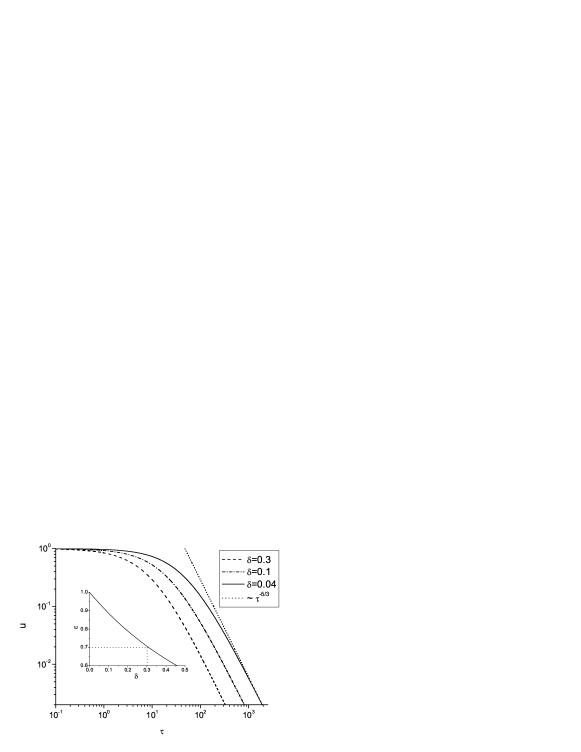
Figure 1: Evolution of the dimensionless granular temperature $u(\tau)=T(\tau)/T(0)$, as it follows from the numerical solution of Eqs. (19), for different values of the dissipative parameter $\delta$. Time is measured in the collision units $\tau_{0}$ (see the text). For $\tau\gg 1$ all curves demonstrate the same slope, $u(\tau)\sim\tau^{-5/3}$ (shown by the dotted line), in accordance with the theoretical prediction, Eq. (26). The inset illustrates the dependence (13) of the restitution coefficient $\varepsilon$ on the dissipative parameter $\delta$ for $u=1$ for collisions with the characteristic thermal velocity, that is for $\left|\vec{c}_{12}\cdot\vec{e}\,\right|=1$. The particular value of $\varepsilon=0.7$, discussed below, corresponds to $\delta\simeq 0.3$.

The numerical solution of Eqs. (19) confirms the obtained asymptotic dependence, Eqs. (24)-(26). This is seen in Fig. 1, where the time dependence of the reduced temperature $u(\tau)$ is plotted and in Figs. 2 and 3 (insets). Fig. 1 demonstrates that the larger the dissipative parameter $\delta$, the earlier the asymptotic behavior of $u(\tau)$ is achieved.

The numerical solution for the Sonine coefficients $a_{2}(\tau)$ and $a_{3}(\tau)$, shown in Fig. 2 and 3, corresponds to the initial Maxwellian distribution, $a_{2}(0)=a_{3}(0)=0$. As it follows from the figures, the absolute values of the both coefficients initially increase, reach their maxima $\left|a_{2\max}\right|$ and $\left|a_{3\max}\right|$ and, eventually, decay to zero. In other words, the velocity distribution function for viscoelastic particles evolves towards the Maxwellian. It is interesting to note, that the maxima $\left|a_{2\max}\right|$ and $\left|a_{3\max}\right|$ first increase with the increasing dissipative parameter $\delta$, then saturate at $\delta\simeq 0.15$ and do not anymore grow. The location of the maxima, however, shifts with increasing $\delta$ to later time, Figs. 2 and 3. This illustrates the general tendency – the larger the dissipation parameter, the slower the gas evolution. Again we see that the third Sonine coefficient $a_{3}$ is of the same order of magnitude as $a_{2}$ (although a few times smaller) for all evolution stages.

To understand the observed behavior of the Sonine coefficients, consider the dependence of these coefficients on $\varepsilon$ for a constant restitution coefficient (Fig. 4) and the respective dependence of the restitution coefficient $\varepsilon$ on the dissipative parameter $\delta$ (Fig. 1, inset). For $0<\delta\,<0.15$ [which corresponds to $0.85<\varepsilon<1$, Fig. 1 (inset)] one observes a fast relaxation, on a collision time scale, of the Sonine coefficients $a_{2}$, $a_{3}$ to their maximal values $\left|a_{2\max}\right|$, $\left|a_{3\max}\right|$, roughly corresponding to the respective values for the constant $\varepsilon$. In a course of time the granular temperature $u(\tau)$ decreases and the effective restitution coefficient alters in accordance with decreasing dissipative parameter $\delta^{\prime}(\tau)=\delta\,\left(2u(\tau)\right)^{1/10}$, that is, the effective $\varepsilon$ increases with time. For this interval of $\varepsilon$ ($0.85<\varepsilon<1$) the increasing restitution coefficient implies the decrease of the absolute values of the Sonine coefficients, Fig. 4, which is indeed observed in the evolution of $a_{2}(\tau)$ and $a_{3}(\tau)$. The larger the $\delta$ (i.e. the smaller the effective restitution coefficient), the larger the maxima $\left|a_{2\max}\right|$ and $\left|a_{3\max}\right|$, in accordance with the dependencies $a_{2}(\varepsilon)$ and $a_{3}(\varepsilon)$ depicted in Fig. 4.

Similarly, for $0.15<\delta\,<0.30$ [which corresponds to $0.7<\varepsilon<0.85$, Fig. 1 (inset)] the initial fast relaxation to the related values of $\left|a_{2\max}\right|$ and $\left|a_{3\max}\right|$ first takes place. Then the decreases of $\delta^{\prime}(\tau)$ and the respective increase of the effective $\varepsilon$ causes the increase of the absolute value of $a_{2}(\tau)$, until it reaches the maximum, corresponding to $\delta^{\prime}(\tau)=0.15$ (or $\varepsilon=0.85$), Fig. 4. The further decrease of $\delta^{\prime}(\tau)$ leads to the according decay of $a_{2}(\tau)$, in agreement with the dependence of $a_{2}(\tau)$ shown in Fig. 2. This qualitatively explains the evolution of $a_{2}(\tau)$ and the saturation of its maximum $\left|a_{2\max}\right|$ for $\delta>0.15$. The qualitative behavior of the third Sonine coefficient may be explained analogously.

Figure 2: Evolution of second Sonine coefficient $a_{2}(\tau)$. At the first stage of the evolution $|a_{2}(\tau)|$ increases, then reaches the maximum value $|a_{2\max}|$, and eventually decays to zero. With the increasing dissipation parameter $\delta$ the maximum $|a_{2\max}|$ shifts to later time. The inset shows the asymptotic dependence of $\left|a_{2}(\tau)\right|$ (full line) together with the analytical result (24) (dotted line) for $\delta=0.01$ in the log-log scale.

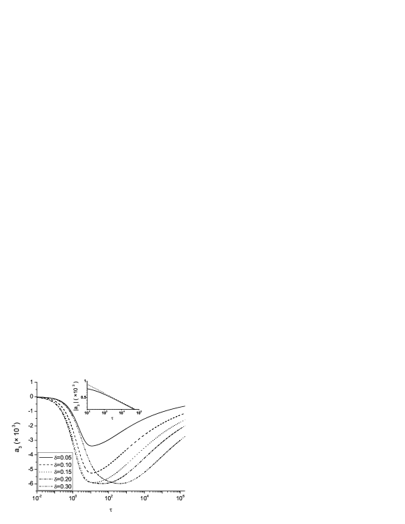
Figure 3: Evolution of the third Sonine coefficient $a_{3}(\tau)$. The inset shows the asymptotic dependence of $\left|a_{3}(\tau)\right|$ (full line) together with the analytical result (25) (dotted line) for $\delta=0.01$ in the log-log scale.

Figure 4: Dependence of the second and third (inset) Sonine coefficients on the restitution coefficient $\varepsilon$ for the case of a constant $\varepsilon$ [1, 17, 18]. Note that $\varepsilon\simeq 0.7$ corresponds to the vanishing $a_{2}$.

It is interesting to note that the observed dependence of $a_{2}(\tau)$ with the new restitution coefficient (13) differs qualitatively for $\delta>0.145$ from that obtained previously for the old restitution coefficient (3). While in the latter case a positive bump at initial time, $\tau\sim 1$ was detected for $\delta>0.145$ [23], in the former case the positive bump appears at much larger $\delta>0.3$, Fig. 5. This is again in agreement with the behavior, expected from the dependence of $a_{2}(\varepsilon)$ for a constant $\varepsilon$: The coefficient $a_{2}$ becomes positive for $\varepsilon<0.7$, which corresponds to $\delta>0.3$, Fig. 1 (inset). Note, however, that with increasing $\delta$ more and more terms in the expansion (13) are to be kept. While for $\delta=0.27$ it suffice to keep terms up to $\delta^{9}$, for $\delta=0.33$ the Sonine coefficients $a_{2}$ computed with the accuracy ${\cal O}(\delta^{9})$, ${\cal O}(\delta^{19/2})$ and ${\cal O}(\delta^{10})$ noticeably differ, Fig. 5. Therefore we conclude that the revised restitution coefficient for a viscoelastic impact (13) may be accurately used up to $\delta=0.3$. The loss of the accuracy in the computation of the Sonine coefficients for larger values of $\delta$ may be a manifestation of the breakdown of the Sonine polynomials expansion, as it has been found previously for a constant restitution coefficient [18]. Similarly as in the case of constant $\varepsilon$ [18], we expect that in the domain of convergence of the Sonine expansion, $\delta<0.3$, the magnitude of the next-order Sonine coefficients $a_{4}$, $a_{5},\,\ldots$ is very small, so that an acceptable accuracy may be achieved with the use of the two coefficients, $a_{2}$ and $a_{3}$ only.

Figure 5: The time dependence of the second Sonine coefficient $a_{2}(\tau)$, computed with a different number of terms in the expansion (13) for the restitution coefficient. The full lines correspond to the accuracy up to ${\cal O}(\delta^{10})$, the dashed lines – up to ${\cal O}(\delta^{19/2})$ and the dotted lines – up to ${\cal O}(\delta^{9})$. Note that for $\delta=0.33$ the accuracy up to ${\cal O}(\delta^{10})$ is insufficient to obtain a reliable convergence.

3 High-velocity tail of the velocity distribution function

The expansion (9) refers to the main part of the velocity distribution, $c\sim 1$, that is, to the velocities, close to the thermal one, $v_{T}$. The high-velocity tail $c\gg 1$ is however exponentially overpopulated [15]. It develops in a course of time, during a first few tens of collisions [30, 31]. For viscoelastic particles the velocity distribution reads for $c\gg 1$ [23]:

$$\tilde{f}(c,\tau)\sim\exp\left(-\varphi(\tau)c\right)\,,$$ (27)

where the function $\varphi(\tau)$ satisfies the equation [23],

$$\dot{\varphi}+\frac{1}{3}\mu_{2}B\varphi=\pi B\,,$$ (28)

with $B$ and $\mu_{2}$ defined previously. Using $\mu_{2}(\tau)$, obtained by the formula manipulation program [1] (see the discussion above), we solve numerically Eq. (28) to obtain $\varphi(\tau)$. In the linear approximation, $\mu_{2}\approx 6.49\,\delta\,\left(2u(\tau)\right)^{1/10}$, the function $\varphi(\tau)$ has the form:

$$\varphi(\tau)=(b/\delta)(1+\tau/\tau_{0})^{\frac{1}{6}}$$ (29)

with $b\approx 1.129$ [1].

Following [30] we neglect the transition region between the main part of the velocity distribution function, $c\sim 1$, and its high-energy part, $c\gg 1$ and write the distribution function as

$$\tilde{f}(c,\tau) =A(\tau)c^{2}\exp(-c^{2})\left(1+a_{2}(\tau)S_{2}(c^{2})+a_{3}(\tau)S_{3}(c^{2})\right)\Theta(c^{*}-c)+$$ (30)

$$+B(\tau)c^{2}\exp\left(-\varphi(\tau)c\right)\Theta(c-c^{*})$$

The coefficients $A(\tau)$, $B(\tau)$ and the threshold velocity $c^{*}$, which separates the main and the tail part of $\tilde{f}(c,\tau)$ can be obtained, using the normalization condition:

$$\int\tilde{f}(c)dc=1$$ (31)

and the continuity condition for the function itself and its first derivative [30]:

$$\tilde{f}(c^{*}-0,\tau)=\tilde{f}(c^{*}+0,\tau)$$ (32)

$$\frac{\partial\tilde{f}(c^{*}-0,\tau)}{\partial c}=\frac{\partial\tilde{f}(c^{*}+0,\tau)}{\partial c}$$ (33)

Substituting Eq. (30) into (31), (32) and (33) we arrive at,

$$\cases{(2c^{*}-\varphi)\left(1+a_{2}S_{2}(c^{*2})+a_{3}S_{3}(c^{*2})\right)=a_{2}\left(2c^{*3}-5c^{*}\right)+a_{3}\left(7c^{*3}-c^{*5}-\frac{35}{4}c^{*}\right)\cr B=A\exp(-c^{*2}+\varphi c^{*})\left(1+a_{2}S_{2}(c^{*2})+a_{3}S_{3}(c^{*2})\right)\cr\left(12\sqrt{\pi}{\rm erf}(c^{*})\exp(c^{*2})-12a_{2}c^{*5}+30a_{2}c^{3*}+35a_{3}c^{*3}-28a_{3}c^{*5}+4a_{3}c^{*7}-24c^{*}\right)\cr\times\frac{A}{48}\exp(-c^{*2})+\frac{B}{\varphi^{3}}\left(2+\varphi c^{*}(2+\varphi c^{*})\right)\exp(-\varphi c^{*})=1}$$ (34)

where $\varphi(\tau)$ is the solution of Eq. (28).

Figure 6: A typical velocity distribution function in a granular gas of viscoelastic particles at $\tau=50$ for $\delta=0.30$ (Eq. (30), solid line), which is represented as a sum of velocity distribution function, obtained in the Sonine polynomial approximation (Eq. (20), dashed line), and the exponential function (Eq. (27), dash-dotted line). For comparison the Maxwellian distribution is also shown (dotted line). The threshold velocity, $c^{*}=4.31$, may be compared with the respective quantity $c^{*}=3.77$ for a gas of particles with a constant restitution coefficient $\varepsilon\simeq 0.71$.

To find the amplitudes $A(\tau)$ and $B(\tau)$ together with the threshold velocity $c^{*}$ the system (34) was solved numerically.

The asymptotic dependence of $c^{*}$ on $\tau$ may be easily found if we take into account that $a_{2}$ and $a_{3}$ are of the same order of magnitude for $\tau\gg 1$, while $\varphi(\tau)\gg 1$ and $c^{*}\gg 1$. Keeping in the first equation in (34) only the largest terms, yields $(2c^{*}-\varphi)a_{3}c^{*\,6}\simeq-a_{3}c^{*\,5}$, which implies that

$$c^{*}(\tau)\simeq\varphi(\tau)/2=(b/2\delta)(1+\tau/\tau_{0})^{1/6}$$ (35)

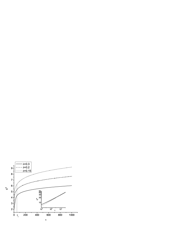
Figure 7: Evolution of the threshold velocity $c^{*}$ in a gas of viscoelastic particles for $\delta=0.3,\,0.2,\,0.15$ (from top to bottom). The corresponding quantities for the case of a constant restitution coefficient are: $c^{*}(\varepsilon\simeq 0.71)=3.77$, $c^{*}(\varepsilon\simeq 0.79)=3.65$ and $c^{*}(\varepsilon\simeq 0.84)=3.60$ [30]. In a course of time the threshold velocity shifts to larger values, that is, the high-energy tail becomes less pronounced. The inset shows the asymptotic dependence of $c^{*}$ (full line) together with the analytical result (35) (dotted line) for $\delta=0.2$ in the log-log scale.

The typical velocity distribution function, computed for $\tau=50$ and $\delta=0.3$ is shown in Fig. 6. The threshold velocity, $c^{*}$ separating the main and the tail part of the velocity distribution reads in this case, $c^{*}\approx 4.31$. The threshold velocity increases with decreasing inelasticity $\delta$ and shifts to larger values at later time, Fig. 7, which means that the high-energy tail becomes less pronounced. Again, we see that in contrast to a gas of particles with a constant restitution coefficient, where the tail of $\tilde{f}(c)$ persists after its relaxation, in a gas of viscoelastic particles the velocity distribution function tends to a Maxwellian.

4 Self-diffusion

Self-diffusion is the only transport process which takes place in a granular gas in a homogeneous cooling state: In spite of the lack of macroscopic currents, a current of tagged particles, identical to the particles of the surrounding gas, but somehow marked, may exist. Moreover, the diffusion coefficient $D$ is directly related to the mobility coefficient of the tagged particles $\kappa$ via the Einstein relation, $\kappa\simeq D/T$, which approximately holds true for granular gases, e.g. [35, 36]. The mean-square displacement of the tagged particles reads [1]

$$\left<\left[\Delta r(\tau)\right]^{2}\right>=\int^{t}D(t^{\prime})dt^{\prime}\,,$$ (36)

where the time-dependent diffusion coefficient (diffusivity) is the solution of the following equation [1]:

$$-\zeta T\frac{\partial D}{\partial T}+D\tau_{v,ad}^{-1}=\frac{T}{m}\,.$$ (37)

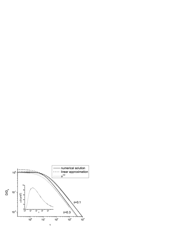
Figure 8: Self–diffusion coefficient as a function of time, measured in the collision units $\tau_{0}$ (see the text). The dissipative parameters, from the top to bottom are $\delta=0.3$ and $\delta=0.1$. $D_{0}$ is the Enskog self-diffusion coefficient in a gas of elastic particles at the initial temperature $T_{0}=T(0)$. The full lines correspond to the complete solution of Eq. (37), while the dashed lines depict the linear approximation to $D$, (42). Note that after a short period of time of about ten collisions, the complete and linear solution become practically indistinguishable. With the dotted lines we show $u^{1/2}(\tau)=\left(T(\tau)/T_{0}\right)^{1/2}$, which is equal to the ratio of two diffusion coefficients for elastic particles at temperatures $T(\tau)$ and $T_{0}$. The plotted ratio $D(\tau)/D_{0}$ clearly tends to $u^{1/2}(\tau)$, which manifests that the self-diffusion in a gas of viscoelastic particles tends to that in a gas of elastic particles. The inset shows the relative deviation $\Delta D=(D-\tilde{D})/D$ of the diffusion coefficient $D$ computed with the use of both Sonine coefficients, $a_{2}$ and $a_{3}$ from the respective value, $\tilde{D}$, obtained with the use of $a_{2}$ only ($\delta=0.3$). Naturally, the location of maximum of $\Delta D$ coincides with that of $\left|a_{3}(t)\right|$, Fig. 3.

Here $\zeta=(2/3)B\mu_{2}$ is, as previously, the cooling coefficient and $\tau_{v,ad}$ is the velocity correlation time, which characterizes the time after which the memory about the initial particle velocity is lost; it reads in terms of the distribution function [1]:

$$\tau_{v,ad}^{-1}=\frac{1}{6}v_{T}(t)g_{2}(\sigma)\sigma^{2}n\times$$ (38)

$$~{}~{}~{}~{}~{}~{}~{}~{}~{}\times\int d\vec{c}_{1}\vec{c}_{2}\int d\vec{e}\,\Theta(-\vec{c}_{12}\cdot\vec{e}\,)\left|\vec{c}_{12}\cdot\vec{e}\,\right|\tilde{f}(\vec{c}_{1},t)\tilde{f}(\vec{c}_{2},t)(1-\varepsilon)(\vec{c}_{12}\cdot\vec{e}\,)^{2}\,.$$

With the approximation (20) for $\tilde{f}(\vec{c},t)$ $\tau_{v,ad}$ was calculated up to $\delta^{10}$, using the formula manipulation program, described in [1]. Here we present for illustration only its linear with respect to $a_{2}$, $a_{3}$ and $\delta^{\prime}$ part:

$$\frac{\tau_{v,ad}}{\tau_{E}(0)}=\left(1+\frac{3}{16}a_{2}+\frac{1}{64}a_{3}\right)-\sqrt{2\pi}\omega_{0}\left(\frac{1}{8}+\frac{3}{100}a_{2}+\frac{1}{500}a_{3}\right)\delta^{\prime}(\tau)$$ (39)

Here $\tau_{E}(0)$ is the Enskog velocity correlation time of elastic particles at initial time $\tau=0$:

$$\tau_{E}^{-1}(0)=\frac{8}{3}\sqrt{\frac{\pi T(0)}{m}}n\sigma^{2}g_{2}\,.$$ (40)

Using the obtained expressions for $\mu_{2}$ and $\tau_{v,ad}$ up to ${\cal O}(\delta^{10})$, we solve Eq. (37) numerically and compute the diffusion coefficient $D(\tau)$. In Fig. 8 the ratio of $D(\tau)/D_{0}$ is plotted, where

$$D_{0}=\tau_{E}(0)T(0)/m\,,$$ (41)

is the Enskog self-diffusion coefficient for a gas of elastic particles at initial temperature $T(0)$. As it is clearly seen from the figure, the diffusion coefficient decreases with time in a way, that the ratio $D(\tau)/D_{0}$ approaches $u^{1/2}(\tau)=\left(T(\tau)/T(0)\right)^{1/2}$ – the ratio of the two diffusion coefficients for elastic particles at the current temperature $T(\tau)$ and the initial temperature $T(0)$. Hence in a course of time the self-diffusion in a gas of viscoelastic particles tends to that in a gas of elastic particles.

In the linear approximation with respect to the small dissipative parameter $\delta$ one can obtain an analytical expression for $D(\tau)$. Keeping only first-order terms in the expressions for $\mu_{2}$, $a_{2}$, $a_{3}$ and $\tau_{v,ad}$ and substituting them into Eq. (37) yields the diffusion coefficient:

$$D=D_{0}u^{1/2}(\tau)\left(1+\frac{4239}{16000}\,\omega_{0}\,\sqrt{\frac{2}{\pi}}\,\delta^{\prime}\right)\,,$$ (42)

where, as previously, $\delta^{\prime}=\delta\left(2u(\tau)\right)^{1/10}$ and $\omega_{0}\approx 6.485$. Note that due to the account of the third Sonine coefficient in $\mu_{2}$ and $\tau_{v,ad}$ the linear approximation (42) for $D(\tau)$ differs from the previously obtained result [1].

The linear approximation (42) is compared in Fig. 8 with the complete numerical solution. As it follows from the figure, after about ten collision per particle the two solution become practically indistinguishable. As it may be seen from the inset of Fig. 8, the impact of the third Sonine coefficient on the behavior of self-diffusion coefficient is rather small even for the large value of dissipation parameter $\delta=0.3$.

5 Conclusion

We study evolution of a granular gas of viscoelastic particles in a homogeneous cooling state. We use a new expression for the restitution coefficient $\varepsilon$, which accounts for the delayed recovery of the particle material at a collision and allows to model collisions with much larger dissipation, as compared to previously available result for $\varepsilon$. We analyze the velocity distribution function and the self-diffusion coefficient. To describe the deviation of the velocity distribution function from the Maxwellian we use the Sonine polynomial expansion. In contrast to the commonly used approximation, which neglects all terms in the Sonine expansion beyond the second one, we consider explicitly the third Sonine coefficient. We detect a complicated evolution of this coefficient and observe that it is of the same order of magnitude, with respect to the (small) dissipative parameter $\delta$, as the second coefficient. This contradicts the existing hypothesis [34], that the subsequent Sonine coefficients $a_{2}$, $a_{3}\ldots$, $a_{k}$ are of an ascending order of some small parameter, characterizing particles inelasticity. Similarly as for the case of a constant restitution coefficient, we obtain an indication of divergence of the Sonine expansion for large dissipation, $\delta>0.3$. For the asymptotic long-time behavior we derive analytical expressions for both Sonine coefficients, which agree well with the numerical data.

Using the obtained third Sonine coefficient we compute the self-diffusion coefficient $D$ and derive an analytical expression for $D$ in the linear, with respect to $\delta$, approximation. We show that the complete solution approaches the approximate analytical solution after a transient time of about ten collisions per particle. We observe, that in spite of the importance of $a_{3}$ for an accurate description of the velocity distribution function, its impact on $D$ is rather small.

We also study the evolution of the high-energy tail of the velocity distribution. Using the equation for the time-dependent slope of the tail and the obtained Sonine coefficients we find the amplitude of the tail and the threshold velocity, which demarcates the main part of the velocity distribution and the high-energy tail. We find the analytical expression for the asymptotic behavior of the threshold velocity, which agrees well with numerics, and observe, that in a course of time it shifts to larger values; this implies that the high-velocity tail becomes less pronounced.

Such behavior of the threshold velocity, of the Sonine coefficients and of the coefficient of self-diffusion, naturally, manifests that the properties of the system tend to those of a gas of elastic particles; our theory quantifies evolution towards this limit.

References

- [1] Brilliantov N V and Pöschel T 2004 Kinetic theory of Granular Gases (Oxford University Press)
- [2] Goldhirsch I 2003 Annual Review of Fluid Mechanics 35 267
- [3] Hinrichsen H, Wolf D E 2004 The Physics of Granular Media Berlin: Wiley
- [4] Pöschel T and Luding S 2001 Granular Gases 564 of Lecture Notes in Physics Berlin: Springer
- [5] Pöschel T and Brilliantov N V 2003 Granular Gas Dynamics 624 of Lecture Notes in Physics Berlin: Springer
- [6] Goldsmit W 1960 The Theory and Physical Behavior of Colliding Solids (London: Arnold)
- [7] Bridges F G, Hatzes A and Lin D N C 1984 Nature 309 333
- [8] Kuwabara G, Kono K 1987 J. Appl. Phys. Part 1 26 1230
- [9] Tanaka T, Ishida T and Tsuji Y 1991 it Trans. Jap. Soc. Mech. Eng. 57 456
- [10] Ramirez R, Pöschel T, Brilliantov N V and Schwager T 1999 Phys. Rev. E 60 4465
- [11] Brilliantov N V, Spahn F, Hertzsch J-M, Poeschel T 1996 Phys. Rev. E. 53 5382
- [12] Morgado W A M and Oppenheim I 1997 Phys. Rev. E 55 1940
- [13] Brilliantov N V, Albers N, Spahn F and Poeschel T 2007 Phys. Rev. E 76 051302
- [14] Schwager T and Pöschel T 1998 Phys. Rev. E 57 650
- [15] Esipov S E and Pöschel T 1997 J. Stat. Phys. 86 1385
- [16] Goldshtein A and Shapiro M 1995 J. Fluid. Mech. 282 75
- [17] van Noije T P C and Ernst M H 1998 Granular Matter 1 57
- [18] Brilliantov N V and Pöschel T 2006 Europhys. Lett. 74 424
- [19] Brey J J, Cubero D and Ruiz-Montero M J 1996 Phys. Rev. E 54 3664
- [20] Montanero J M and Santos A 1999 Granular Matter 2 53
- [21] Nakanishi H 2003 Phys. Rev. E 67 010301R
- [22] Noskowicz S H, Bar-Lev O, Serero D, Goldhirsch I 2007 Europhys. Lett. 79 60001
- [23] Brilliantov N V and Pöschel T 2000 Phys. Rev. E 61 5573
- [24] Brilliantov N V and Pöschel T 2003 Phys. Rev. E 67 061304
- [25] Pöschel T and Brilliantov N V 2003 in [5] p.131
- [26] McNamara S 1993 Physics of Fluids A 5 3056
- [27] Goldhirsch I and Zanetti G 1993 Phys. Rev. Lett. 70 1619
- [28] Brito R and Ernst M H 1998 Europhys. Lett. 43 497
- [29] Brilliantov N V, Saluena C, Schwager T and Poeschel T 2004 Phys. Rev. Lett. 93 134301
- [30] Pöschel T, Brilliantov N V and Formella A 2006 Phys. Rev. E 74 041302
- [31] Pöschel T, Brilliantov N V and Formella A 2007 Int. J. Mod. Phys. C 18 701
- [32] Schwager T and Pöschel T 2008 Phys. Rev. E 78 051304
- [33] Bodrova A S and Brilliantov N V 2009 Moscow University Physics Bulletin 64 131
- [34] Huthmann M, Orza J A and Brito R 2000 Granular Matter 2 189
- [35] Barrat A , Loreto V and Puglisi A 2004 Physica A 334 513
- [36] Garzo V 2004 Physica A 343 105