A model of ballistic aggregation and fragmentation

Abstract

A simple model of ballistic aggregation and fragmentation is proposed. The model is characterized by two energy thresholds, $E_{\rm agg}$ and $E_{\rm frag}$, which demarcate different types of impacts: If the kinetic energy of the relative motion of a colliding pair is smaller than $E_{\rm agg}$ or larger than $E_{\rm frag}$, particles respectively merge or break; otherwise they rebound. We assume that particles are formed from monomers which cannot split any further and that in a collision-induced fragmentation the larger particle splits into two fragments. We start from the Boltzmann equation for the mass-velocity distribution function and derive Smoluchowski-like equations for concentrations of particles of different mass. We analyze these equations analytically, solve them numerically and perform Monte Carlo simulations. When aggregation and fragmentation energy thresholds do not depend on the masses of the colliding particles, the model becomes analytically tractable. In this case we show the emergence of the two types of behavior: the regime of unlimited cluster growth arises when fragmentation is (relatively) weak and the relaxation towards a steady state occurs when fragmentation prevails. In a model with mass-dependent $E_{\rm agg}$ and $E_{\rm frag}$ the evolution with a cross-over from one of the regimes to another has been detected.

1 Introduction

Collision-induced aggregation and fragmentation are ubiquitous processes underlying numerous natural phenomena. For a gentle collision with a small relative velocity, colliding particles can merge; a violent collision with a large relative velocity can cause fragmentation. For intermediate relative velocities, particles usually rebound. These collisions may still be irreversible — the kinetic energy could be lost in inelastic collisions. Important examples of such systems are dust agglomerates in the Earth atmosphere or in interstellar dust clouds and proto-planetary discs [1, 2, 3, 4]. Another example is dynamic ephemeral bodies in planetary rings, see e.g. [5, 6, 7]. A comprehensive description of the aggregation and fragmentation kinetics in such systems is very complicated. Therefore it is desirable to develop idealized models that involves three types of collisions in the simplest possible way.

The understanding of the ballistic-controlled reactions is still quite incomplete [8]. Ballistic aggregation has attracted most attention (see [3, 4, 9, 10, 11, 12, 13, 14] and references therein) and a few studies were also devoted to ballistic fragmentation (see [15, 16, 17, 18]). The situation with aggregation and fragmentation operating simultaneously has been analyzed only in a very special case when all particles have the same relative velocity and the after-collision fragment mass distribution obeys a power-law [7]. Moreover, studies of pure ballistic fragmentation are usually based on the assumption that all particles may split independently on their mass and relative velocity between the colliding grains [16, 17]. In reality, the type of an impact strongly depends on the relative velocity [4]; furthermore, the agglomerates are comprised of primary particles (“grains”) that cannot split into smaller fragments [5, 6]. The fragmentation model with the splitting probability depending on energy has been studied in [19]; this model, however, does not consider ballistic impacts of many particles, but rather an abstract process of a successive fragmentation of one body with a random distribution of the bulk energy between fragments.

In this paper we propose a model of ballistic aggregation and fragmentation which accounts for three types of collisions depending on masses and relative velocity of a colliding pair. In section 2 we introduce the model, write the Boltzmann equation for the joint mass-velocity distribution function, and deduce from the Boltzmann equation the rate equations for concentrations of various mass species. Section 3 is devoted to the theoretical analysis of rate equations. Numerical verification of theoretical results and simulation results in situations intractable theoretically is given in section 4. The last section 5 concludes the paper.

2 The model

Consider a system comprised of primary particles (monomers) of mass $m_{1}$ and radius $r_{1}$, which aggregate to form clusters of $2,\,3,\ldots,k,\ldots$ monomers with masses $m_{k}=km_{1}$. In some applications (e.g. in modeling of dynamic ephemeral bodies [5, 6]) it is appropriate to consider clusters as objects with fractal dimension $D$; for compact clusters $D=3$. The characteristic radius of an agglomerate containing $k$ monomers scales with mass as $r_{k}\sim r_{1}k^{1/D}$. We assume that when the kinetic energy of two colliding clusters in the center-of-mass reference frame (the “relative kinetic energy” in short) is less than $E_{\rm agg}$, they merge. In this case a particle of mass $(i+j)m_{1}$ is formed. If the relative kinetic energy is larger than $E_{\rm agg}$, but smaller than $E_{\rm frag}$, the colliding particles rebound without any change of their properties. Finally, if the relative kinetic energy exceeds $E_{\rm frag}$, one of the particles (we assume that the larger one) splits into two fragments. We denote $p_{i,k-i}$ the probability that a particle of mass $k$ splits into particles of masses $i$ and $k-i$. Obviously, $\sum_{i}p_{i,k-i}=1$ and $p_{i,k-i}=0$ if $k\leq i$.

We restrict ourselves to dilute and spatially uniform systems. Let $f_{i}\equiv f(\vec{v}_{i},t)$ be the mass-velocity distribution function which gives the concentration of particles of mass $m_{i}$ with the velocity $\vec{v}_{i}$ at time $t$. The mass-velocity distribution function evolves according to the Boltzmann equation

$$\frac{\partial}{\partial t}f_{k}\left(\vec{v}_{k},t\right)=I^{\rm agg}_{k}+I^{\rm reb}_{k}+I^{\rm frag}_{k}\,,$$ (1)

where $I^{\rm agg}_{k}$, $I^{\rm reb}_{k}$ and $I^{\rm frag}_{k}$ are respectively the collision integrals describing collisions leading to aggregation, rebound, and fragmentation. The first integral reads

$$I^{\rm agg}_{k}(\vec{v}_{k}) = \frac{1}{2}\sum_{i+j=k}\sigma_{ij}^{2}\int d\vec{v}_{i}\int d\vec{v}_{j}\int d\vec{e}\,\Theta\left(-\vec{v}_{ij}\cdot\vec{e}\,\right)\left|\vec{v}_{ij}\cdot\vec{e}\,\right|\times$$

$$\times f_{i}\left(\vec{v}_{i}\right)f_{j}\left(\vec{v}_{j}\right)\Theta\left(E_{\rm agg}-E_{ij}\right)\delta(m_{k}\vec{v}_{k}-m_{i}\vec{v}_{i}-m_{j}\vec{v}_{j})$$

$$- \sum_{j}\sigma_{kj}^{2}\int d\vec{v}_{j}\int d\vec{e}\,\Theta\left(-\vec{v}_{kj}\cdot\vec{e}\,\right)\left|\vec{v}_{kj}\cdot\vec{e}\,\right|\times$$

$$\times f_{k}\left(\vec{v}_{k}\right)f_{j}\left(\vec{v}_{j}\right)\Theta\left(E_{\rm agg}-E_{kj}\right)\,.$$

Here $\sigma_{ij}=r_{1}\left(i^{1/D}+j^{1/D}\right)$ is the sum of radii of the two clusters, while $m_{k}=m_{i}+m_{j}$ and $m_{k}\vec{v}_{k}=\vec{v}_{i}m_{i}+m_{j}\vec{v}_{j}$, due to the conservation of mass and momentum. We also introduce the relative velocity, $\vec{v}_{ij}=\vec{v}_{i}-\vec{v}_{j}$, the reduced mass, $\mu_{ij}=m_{i}m_{j}/(m_{i}+m_{j})$, and the relative kinetic energy, $E_{ij}=\frac{1}{2}\mu_{ij}v_{ij}^{2}$. The unit vector $\vec{e}$ specifies the direction of the inter-center vector at the collision instant. The factors in the integrand in Eq. (2) have their usual meaning (see e.g. [20]): $\sigma_{ij}^{2}\left|\vec{v}_{ij}\cdot\vec{e}\,\right|$ defines the volume of the collision cylinder, $\Theta\left(-\vec{v}_{ij}\cdot\vec{e}\,\right)$ selects only approaching particles and $\Theta\left(E_{\rm agg}-E_{ij}\right)$ guarantees that the relative kinetic energy does not exceed $E_{\rm agg}$ to cause the aggregation. The first sum in the right-hand side of Eq. (2) refers to collisions where a cluster of mass $k$ is formed from smaller clusters of masses $i$ and $j$, while the second sum describes the collisions of $k$-clusters with all other aggregates.

For collisions leading to fragmentation we have

$$I^{\rm frag}_{k}(\vec{v}_{k}) = \sum_{j}\sum_{i\leq j}p_{k,j-k}\left(1-\frac{1}{2}\delta_{i,j}\right)\sigma_{ij}^{2}\int d\vec{v}_{j}\int\!d\vec{v}_{i}\int d\vec{e}\,\Theta\left(-\vec{v}_{ij}\cdot\vec{e}\,\right)\times$$

$$\times \left|\vec{v}_{ij}\cdot\vec{e}\,\right|f_{j}\left(\vec{v}_{j}\right)f_{i}\left(\vec{v}_{i}\right)\Theta\left(E_{ij}-E_{\rm frag}\right)\Delta(\vec{v}_{i},\,\vec{v}_{j},\,\vec{v}_{k})$$

$$- \sum_{i\leq k}\left(1-\frac{1}{2}\delta_{i,k}\right)\sigma_{ki}^{2}\int d\vec{v}_{i}\int d\vec{e}\,\Theta\left(-\vec{v}_{ki}\cdot\vec{e}\,\right)\left|\vec{v}_{ki}\cdot\vec{e}\,\right|\times$$

$$\times f_{k}\left(\vec{v}_{k}\right)f_{i}\left(\vec{v}_{i}\right)\Theta\left(E_{ki}-E_{\rm frag}\right)\,,$$

where $m_{j}=m_{k}+m_{j-k}$ and we use the abbreviation, $\Delta(\vec{v}_{i},\,\vec{v}_{j},\,\vec{v}_{k})=\delta(m_{j}\vec{v}_{j}+m_{i}\vec{v}_{i}-m_{k}\vec{v}_{k}-m_{k-j}\vec{v}_{k-j}^{\,\prime}+m_{i}\vec{v}_{i}^{\,\prime})$ for the factor which guarantees the momentum conservation at the collision. The after-collisional velocities $\vec{v}_{k-j}^{\,\prime}$ and $\vec{v}_{i}^{\,\prime}$ are determined by a particular fragmentation model. The first sum in Eq. (2) describes the collision of particles of mass $i$ and $j$ ($j\geq k$, $j\geq i$) with the relative kinetic energy above the fragmentation threshold $E_{\rm frag}$. The larger particle, i.e. the particle of mass $j$, splits with the probability $p_{k,j-k}$ into two particles of mass $k$ and $j-k$ thereby giving rise to a particle of mass $k$. The second sum describes the opposite process, when particles of mass $k$ break in collisions with smaller particles. In the present study we do not need an explicit expression for the velocities $\vec{v}_{k-j}^{\,\prime}$ and $\vec{v}_{i}^{\,\prime}$ of the fragments. We do not also need an expression for the collision integral $I^{\rm reb}_{k}$; it has the usual form (see e.g. [20]) with a slight modification to account for the requirement that the relative kinetic energy $E_{ij}$ belongs to the interval $(E_{\rm agg}\,<E_{ij}<\,E_{\rm frag})$.

Thus we have a mixture of particles of different masses and each species generally has its own temperature. For this (granular) mixture we write

$$n_{i}=\int d\vec{v}_{i}f_{i}(\vec{v}_{i})\,,\qquad\qquad~{}~{}N=\sum_{i}n_{i}$$ (4)

where $n_{i}$ is the number density (concentration) of particles of mass $i$ and $N$ is the total number density. Using the mean kinetic energy of different species one can also define the partial granular temperatures $T_{i}$ for clusters of mass $i$ and effective temperature $T$ of the mixture [21]. We assume that the distribution function $f_{i}(\vec{v}_{i},t)$ may be written as [4, 14, 21]

$$f_{i}(\vec{v}_{i},t)=\frac{n_{i}(t)}{v_{0,\,i}^{3}(t)}\phi_{i}(\vec{c}_{i})\,,\qquad\vec{c}_{i}\equiv\frac{\vec{v}_{i}}{v_{0,\,i}}\,,$$ (5)

where $v_{0,\,i}^{2}(t)=2T_{i}(t)/m_{i}$ is the thermal velocity and $\phi(c_{i})$ the reduced distribution function. For the force-free granular mixtures the velocity distribution functions of the components are not far from the Maxwellian distribution [21], which reads in terms of the reduced velocity $\vec{c}=\vec{v}/v_{T}$,

$$\phi_{M}(\vec{c})=\pi^{-3/2}\exp(-c^{2})\,.$$ (6)

The equipartition between different components may, however, break down, in the sense that the partial temperatures $T_{i}$ are not equal and differ from the effective temperature $T$ [21]. Here we ignore the deviation from the Maxwellian distribution and possible violation of the equipartition and use the approximation, $\phi_{i}(c_{i})\approx\phi_{M}(c_{i})$ and $T_{i}\approx T$ for all $i$. We also assume that the temperature of the system does not depend on time. This is formally inconsistent within the Boltzmann equation (1), yet in many applications the temperature is approximately constant on a astronomical time scale, e.g. this happens in planetary rings where the viscous heating due to the shearing mode of the particle orbital motion keeps the granular temperature constant [22, 4]. The consistent approach would be to modify the Boltzmann equation to take into account gradients of the local hydrodynamic velocity, which will result in additional terms in the velocity distributions $f_{i}$, proportional to these gradients. If we assume that such gradients are very small but still sufficient to support constant temperature due to viscous heating, we can neglect the small corrections to the distribution functions and approximate them with a gradient-free form (5).

Integrating Eq. (1) over $\vec{v}_{k}$ we obtain the equations for the zero-order moments of the velocity distribution functions $f_{k}$, that is, for the concentrations $n_{k}$. Taking into account that collisions resulting in rebounds do not change the concentrations of different species and using (2)–(2) together with (4)–(6) we arrive at rate equations

$$\frac{d}{dt}n_{k} = \frac{1}{2}\sum_{i+j=k}C_{i,j}n_{i}n_{j}-n_{k}\sum_{i=1}^{\infty}C_{k,i}n_{i}+\sum_{j=k+1}^{\infty}\!\sum_{i=1}^{j}A_{i,j}n_{i}n_{j}\left(1-\!\frac{1}{2}\delta_{i,j}\right)p_{k,j-k}$$ (7)

$$- n_{k}(1-\delta_{1k})\sum_{i=1}^{k}A_{k,i}n_{i}\left(1-\frac{1}{2}\delta_{i,k}\right)\,,$$

with rates given by

$$C_{i,j}=2\sigma_{ij}^{2}\left(\frac{2T\pi}{\mu_{ij}}\right)^{1/2}\left(1-\left(1+\frac{E_{\rm agg}}{T}\right)e^{-E_{\rm agg}/T}\right)$$

$$A_{i,j}=2\sigma_{ij}^{2}\left(\frac{2T\pi}{\mu_{ij}}\right)^{1/2}e^{-E_{\rm frag}/T}\,.$$ (8)

It is useful to verify that the above kinetic equation (7) fulfills the condition of mass conservation, $\sum_{k}km_{1}n_{k}=M={\rm const.}$, where $M$ is the total mass density.

The probability of splitting $p_{ik}$ depends on geometric and mechanical properties of the aggregates and generally it is quite complicated. For concreteness we focus on splitting into (almost) equal fragments. Namely, we assume that a particle of mass $2km_{1}$ splits into two equal halves, while a particle of mass $(2k+1)m_{1}$ splits into particles of mass $km_{1}$ and $(k+1)m_{1}$. For this choice of the splitting probability, the kinetic equation reads

$$\frac{d}{dt}n_{k} = \frac{1}{2}\sum_{i+j=k}C_{i,j}n_{i}n_{j}-n_{k}\sum_{i=1}^{\infty}C_{k,i}n_{i}-n_{k}\sum_{i=1}^{k}A_{k,i}n_{i}\left(1-\delta_{k,i}/2\right)$$ (9)

$$+ 2\sum_{i=1}^{2k}A_{2k,i}n_{2k}n_{i}\left(1-\delta_{2k,i}/2\right)+\sum_{i=1}^{2k+1}A_{2k+1,i}n_{2k+1}n_{i}\left(1-\delta_{2k+1,i}/2\right)$$

$$+ \sum_{i=1}^{2k-1}A_{2k-1,i}n_{2k-1}n_{i}\left(1-\delta_{2k-1,i}/2\right)\,.$$

In the next sections we study this model theoretically and numerically.

3 Theoretical analysis

To understand the qualitative behavior it is instructive to start with the simplest model which allows an analytical treatment.

3.1 Constant rates

Consider first the model with constant rates $A_{i,j}$ and $C_{i,j}$. Without loss of generality we can choose these rates to be

$$C_{i,j}=2\,,\qquad\qquad A_{i,j}=2\lambda\,,$$ (10)

The parameter $\lambda$ quantifies the relative intensity of fragmentation with respect to aggregation. Fragmentation prevails when $\lambda>1$ while aggregation wins in the opposite case of $\lambda<1$. If $\lambda=1$ two processes are in a balance.

Even in this simple case we still ought to analyze a cumbersome system of infinitely many equations. To gain insight it is useful to consider the evolution of the total density $N=\sum n_{k}$. (In many problems involving aggregation and fragmentation this quantity satisfies a simple equation that does not contain other densities.) Summing up all equations (9) we obtain

$$\dot{N}=-(1-\lambda)N^{2}-\lambda n_{1}^{2}$$ (11)

which has indeed a neat form, although it additionally involves the density of monomers. This density evolves according to

$$\dot{n}_{1}=-2n_{1}N+2\lambda\left[n_{2}(2n_{1}+n_{2})+n_{3}(n_{1}+n_{2})+\frac{1}{2}n_{3}^{2}\,\right]\,.$$ (12)

Although we do not have a closed system we can already reach some qualitative conclusions. Equation (11) indicates that two regimes are possible. If $\lambda<1$, i.e. when aggregation prevails, the system continues to evolve leading to formation of larger and larger clusters; when $\lambda>1$, one expects that the system reaches a steady state. We now analyze these situations in more detail.

3.1.1 Unlimited cluster growth, $\lambda<1$

In this case larger and larger clusters will arise. Since the total mass is conserved, one expects that the concentration of small clusters will rapidly decrease. Therefore, $n_{1}\ll N$ when $t\gg 1$ and therefore one can omit the second term on the right-hand side of (11). Similarly one can keep only the first term on the right-hand side of (12). This leads to the simplified equations

$$\dot{N}\simeq-(1-\lambda)N^{2},\qquad\qquad\dot{n}_{1}\simeq-2n_{1}N$$ (13)

which are solved to yield the large time behavior:

$$N\simeq\frac{1}{(1-\lambda)t}$$ (14)

$$n_{1}\sim t^{-2/(1-\lambda)}$$ (15)

Further, one anticipates that the density distribution approaches the scaling form

$$n_{k}\simeq t^{-2z}\Phi(x),\quad x=\frac{k}{t^{z}}$$ (16)

in the scaling limit $t\to\infty$, $k\to\infty$, with the scaled mass $x=k/t^{z}$ kept finite. (Here $z$ is the dynamic exponent characterizing the average mass: $\langle k\rangle\sim t^{z}$.) The scaling form agrees with mass conservation: $\sum kn_{k}\simeq\int dx\,x\Phi(x)$ is manifestly time-independent.

The exponent $z$ can be found from the known asymptotic behavior of $N(t)$. Indeed, writing

$$N=\sum_{k\geq 1}n_{k}\simeq t^{-z}\int_{0}^{\infty}dx\,\Phi(x)\sim t^{-z}$$

and matching this with already known asymptotic behavior (14) we conclude that $z=1$. If we further assume that $\Phi(x)\sim x^{\mu}$ for $x\ll 1$ and combine this asymptotic with $z=1$ and the scaling ansatz (16) we obtain $n_{1}\sim t^{-2}\,t^{-\mu}$. Matching with (15) we get $\mu=2\lambda/(1-\lambda)$. Therefore

$$n_{k}\sim\frac{1}{t^{2}}\,\left(\frac{k}{t}\right)^{2\lambda/(1-\lambda)}$$ (17)

when $k\ll t$. Obviously, the above equation implies the asymptotic time dependence $n_{k}\sim t^{-2/(1-\lambda)}$ and the mass dependence $n_{k}\sim k^{2\lambda/(1-\lambda)}$ for $x=k/t\ll 1$.

3.1.2 Relaxation to a steady state, $\lambda>1$

For $\lambda>1$ the system evolves to a steady state with constant concentration of clusters. In this case $\dot{n}_{k}=\dot{N}=0$ and Eq. (11) yields,

$$n_{1}=N\sqrt{1-\lambda^{-1}}$$ (18)

The densities $n_{k}$ rapidly decay with $k$. Therefore $n_{2k}\ll n_{k}$ for $k\gg 1$ and the governing equations (9) for the stationary concentrations simplify to

$$\sum_{i=1}^{k-1}n_{i}n_{k-i}-2(1+\lambda)n_{k}N=0$$ (19)

where we have approximated a finite sum up to $k\gg 1$ by an infinite sum and ignore the terms containing $n_{2k},n_{2k\pm 1}$. The above equation is supposed to be valid for large $k$; it is certainly invalid for $k=1$ when the right-hand side does not vanish. The qualitative form of the large $k$ asymptotic behavior is determined by the mathematical structure of (19). To extract this asymptotic let us consider the simplest version when Eq. (19) is valid for all $k\geq 2$. Specifically, let us probe the model

$$\sum_{i=1}^{k-1}n_{i}n_{k-i}-2(1+\lambda)n_{k}N=-(1+2\lambda)N\delta_{k,1}\,,$$ (20)

where the amplitude $(1+2\lambda)$ was chosen to set $N=1$. (For model (20), this choice merely sets the overall amplitude.)

The infinite system (20) forms a recurrence and therefore it is solvable. Introducing the generating function

$$\mathcal{N}(z)=\sum_{k\geq 1}n_{k}\,z^{k}$$ (21)

we recast (20) into a quadratic equation

$$\mathcal{N}^{2}-2(1+\lambda)\mathcal{N}+(1+2\lambda)z=0$$ (22)

which is solved to yield

$$\mathcal{N}=(1+\lambda)-\sqrt{(1+\lambda)^{2}-(1+2\lambda)z}$$ (23)

Expanding ${\cal N}(z)$ we arrive at

$$n_{k}=\frac{1+\lambda}{\sqrt{4\pi}}\left[1-\frac{1}{(1+\lambda)^{2}}\right]^{k}\,\frac{\Gamma(k-\frac{1}{2})}{\Gamma(k+1)}$$ (24)

From this solution one gets $n_{1}=(\lambda+1/2)/(\lambda+1)$, which of course directly follows from Eq. (20) as well. For large $k$, equation (24) simplifies to

$$n_{k}\simeq\frac{1+\lambda}{\sqrt{4\pi}}\,k^{-3/2}\left[1-\frac{1}{(1+\lambda)^{2}}\right]^{k}$$ (25)

We considered other tractable versions when Eq. (19) is exact above a certain threshold, $k\geq\kappa+1$, while for $k=1,\ldots,\kappa$ we use the same modification as in Eq. (20) for $k=1$. In this case instead of (22) one gets $\mathcal{N}^{2}-2(1+\lambda)\mathcal{N}+P(z)=0$ with $P(z)=A_{1}z+\ldots+A_{\kappa}z^{\kappa}$. The root of $P(z)=(1+\lambda)^{2}$ closest to the origin is positive [one can show that it exceeds unity, $z_{*}>1$] and non-degenerate. Expanding the generating function $\mathcal{N}=1+\lambda-\sqrt{(1+\lambda)^{2}-P(z)}$ leads to the asymptotic $n_{k}\sim k^{-3/2}z_{*}^{-k}$. The above argument favors the asymptotic behavior

$$n_{k}\simeq Ak^{-3/2}e^{-\gamma k}$$ (26)

This asymptotic form is universal and only the parameters $A,\,\gamma$ depend on the specificity of the model, that is on the parameter $\lambda$.

It is impossible to determine $A,\,\gamma$ since models like (20) are uncontrolled approximations. Let us still use such models and choose the simplest one which obeys the exact relation of Eq. (18). The model (20) is inappropriate as it fails to satisfy (18): $(\lambda+1/2)/(\lambda+1)>\sqrt{1-\lambda^{-1}}$. Modifying Eq. (19) at $k=1,2$ yields (we still set $N=1$)

$$\sum_{i+j=k}n_{i}n_{j}-2(1+\lambda)n_{k}=-q\delta_{k,1}-(2\lambda+1-q)\delta_{k,2}$$ (27)

with

$$q=2(1+\lambda)\sqrt{1-\lambda^{-1}}$$

ensuring the validity of (18). The same approach as before gives (26) with $A$ and $\gamma$. In particular,

$$\gamma=\ln\left[(1+\lambda)\,\frac{\sqrt{1-\lambda^{-1}+\Lambda}-\sqrt{1-\lambda^{-1}}}{\Lambda}\right]$$ (28)

where we have used the short-hand notation $\Lambda=1+2\lambda-2(1+\lambda)\sqrt{1-\lambda^{-1}}$. For $\lambda=2$ (which we have studied numerically) one gets

$$\gamma=0.495156\ldots$$ (29)

This is an uncontrolled approximation, of course. Interestingly, the result is rather close to the numerically obtained value $\gamma\approx 0.465$.

3.2 Mass-independent energy thresholds

We now turn to the analysis of the situation when aggregation and fragmentation energy thresholds $E_{\rm agg}$ and $E_{\rm frag}$ are constant. In this case the total density of clusters evolves according to

$$\dot{N}=-\frac{1}{2}(1-\lambda)\sum_{i=1}^{\infty}\sum_{j=1}^{\infty}C_{i,j}n_{i}n_{j}-\frac{1}{2}\lambda C_{1,1}n_{1}^{2}\,,$$ (30)

where $\lambda^{-1}=e^{E_{\rm frag}/T}\left(1-(1+E_{\rm agg}/T\right)e^{-E_{\rm agg}/T})$. This again implies the existence of the two opposite evolution regimes: For $\lambda>1$ the relaxation to a steady state is expected, while for $\lambda<1$ – the regime of the unlimited cluster growth.

The rates $C_{ij}=C(i,j)$ and $A_{ij}=A(i,j)$ differ by a constant factor $\lambda$; moreover, they are homogeneous functions of their arguments:

$$A(ai,aj)=a^{\nu}A(i,j)\,,\qquad\qquad C(ai,aj)=a^{\nu}C(i,j)$$ (31)

with the exponent

$$\nu=\frac{2}{D}-\frac{1}{2}\,,$$ (32)

which follows from the relation for a particles mass $m_{i}=im_{1}$, the cross-section of the collision cylinder, $\sigma_{ij}^{2}\sim\left(i^{1/D}+i^{1/D}\right)^{2}$, and Eqs. (2). Plugging the scaling Ansatz (16) into Eq. (9), taking into account that for $k\gg 1$ the summation may be approximated by integration, and exploiting the homogeneity of the rate kernels, Eq. (31), we obtain (see e.g. [23, 25, 24] for analysis of similar integro-differential equations for the re-scaled mass distribution)

$$\frac{z}{t^{2z+1}}\left(2\Phi(x)+x\Phi^{\,\prime}(x)\right)=\frac{1}{t^{(3-\nu)z}}\,\int_{0}^{\infty}dy\Phi(y)\left[(C_{x,y}+A_{x,y})\Phi(x)\right.$$ (33)

$$~{}~{}~{}~{}~{}~{}~{}~{}~{}~{}~{}~{}~{}~{}~{}~{}~{}~{}~{}~{}~{}~{}~{}~{}~{}~{}~{}~{}~{}~{}~{}~{}~{}~{}~{}~{}~{}~{}\left.-\frac{1}{2}C_{y,x-y}\Phi(x-y)-4A_{2x,y}\Phi(2x)\right]\,.$$

From Eq. (33) we find the scaling exponent

$$z=\frac{1}{1-\nu}=\left(\frac{3}{2}-\frac{2}{D}\right)^{-1}\,.$$ (34)

Although the scaling theory does not allow to determine the scaling function $\Phi(x)$, one can find the total concentration of clusters from Eq. (34):

$$N(t)\sim t^{-z}\sim t^{-2D/(3D-4)}\,.$$ (35)

Correspondingly, the average clusters mass grows as $\left<k\right>=M/N\sim t^{z}$.

3.3 Dependence of the energy thresholds on masses of colliding particles

In the preceding analysis we have assumed that $E_{\rm agg}$ and $E_{\rm frag}$ do not depend on the mass of colliding particles so that $\lambda_{ij}=A_{ij}/C_{ij}=\lambda$ is constant. In reality, however, such dependence does exist, implying that $\lambda_{ij}$ is a function of $i$ and $j$. Still, if $\lambda_{ij}>1$ or $\lambda_{ij}<1$ for all $i$ and $j$, the qualitative behavior of a system is similar to that for the case of constant $E_{\rm agg}$ and $E_{\rm frag}$: For $\lambda_{ij}>1$ a relaxation to a steady state is expected, while for $\lambda_{ij}<1$ an unlimited cluster growth is observed. The most interesting behavior is expected when $\lambda_{ij}-1$ changes its sign with increasing clusters masses $i$ and $j$. In this case one anticipates a cross-over from one type of evolution to another.

To choose a realistic dependence of $E_{\rm agg}$ and $E_{\rm frag}$ on the masses of colliding particles, one needs more details of the collision process. We shall use the threshold energy for ballistic aggregation that takes into account surface adhesion [26]. In this case

$$E_{\rm agg}(i,j)=E_{\rm agg}^{0}\left(\frac{ij}{i+j}\right)^{\frac{4}{3}}\,,$$ (36)

where $E_{\rm agg}^{0}$ is expressed in terms of the monomer radius, particle surface tension, the Young modulus and the Poisson ratio of the particle material (see [26] for the explicit expression for $E_{\rm agg}^{0}$).

For the energy of fragmentation we assume that it is equal to the energy required to create an additional surface, which may be roughly estimated as twice the area of the equatorial cross-section of the larger particle (recall that the model assumes, that the larger particle in a collision pair breaks down). Hence we adopt the following mass dependence for $E_{\rm frag}$:

$$E_{\rm frag}(ij)=E_{\rm frag}^{0}\left(\theta_{ij}i+\theta_{ji}j\right)^{2}\,,$$ (37)

where $\theta_{ij}=1$ if $i>j$, $\theta_{ij}=0$ if $i<j$ and $\theta_{ii}=1/2$; $E_{\rm frag}^{0}=2\pi\gamma_{s}r_{1}^{2}$, with $\gamma_{s}$ being the surface tension.

4 Numerical simulations

In our numerical studies we apply two different approaches – the solutions of the system of differential equations and the direct modeling of random aggregation and fragmentation processes (with the corresponding rates $C_{i,j}$ and $A_{i,j}$) by means of Monte Carlo (MC) method. In the former case we use $1000$ equations and in the later one $100,000$ monomers (we always used the mono-disperse initial conditions). The approach based on the solution of differential equation has an obvious deficiency as one must approximate an infinite system of equations with a finite one. The MC approach is more time consuming, yet it has an advantage of directly imitating the physical processes in which particles are involved. To model the fragmentation and aggregation kinetics by MC we use the standard Gillespie algorithm [27, 28] (see [29] for the application of this algorithm to the aggregation and fragmentation processes).

The results presented on Figs. 1–11 confirm our theoretical predictions qualitatively and quantitatively. For constant rates two opposite types of evolution have indeed been observed: the relaxation to a steady state for dominating fragmentation ($\lambda>1$) and the unlimited cluster growth when aggregation prevails ($\lambda<1$). Both numerical approaches (the solution of the differential equations and MC) yield very close results.

In Fig. 1 the evolution of the concentration of clusters of different mass is shown for the $\lambda<1$ regime when the cluster growth continues ad infinitum. Note that all concentrations $n_{k}(t)$, except for $n_{1}(t)$ which always decays, initially increase and then decay to zero.

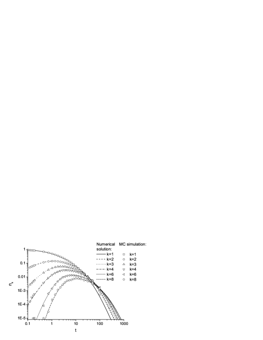
Figure 1: Evolution of cluster concentrations $n_{k}$ in the case of constant rates with $\lambda=0.5$. The lines correspond to the numerical solution of 1000 differential equations, symbols are the results of MC simulation with 100 000 monomers for the monodisperse initial conditions. Note, that while $n_{1}(t)$ always decays, $n_{k}(t)$ initially increase and than decay to zero.

Figure 2 shows that the decay of cluster density $N(t)$ well agrees with the theoretical prediction (14).

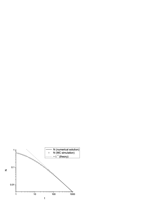
Figure 2: Evolution of the total number of clusters $N$ for the same system as in Fig. 1. The solid line corresponds to the numerical solution of the differential equations, symbols – to the MC simulation and the dotted line shows the theoretical prediction, Eq.  (14), $N(t)\sim t^{-1}$ for $t\gg 1$.

Figures 3, 4 show respectively the asymptotic evolution of cluster concentrations and the distribution of the cluster mass for $x=k/t\ll 1$. The theoretical predictions, Eqs. (15) and (17), are in a good agreement with the simulations.

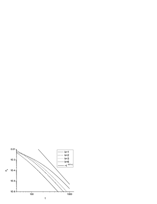
Figure 3: The long-time limit behavior of cluster concentrations $n_{k}$ for the same system as in Fig. 1. In accordance with the theoretical predictions, Eqs. (15) and (17), the cluster concentrations $n_{k}(t)$ decay for $t\gg 1$ with the same slope $t^{-2/(1-\lambda)}\sim t^{-4}$, shown by the solid line.

Relaxation to a steady state in the case when fragmentation dominates ($\lambda>1)$ is illustrated in Fig. 5, while Fig. 6 demonstrates the corresponding stationary cluster mass distribution.

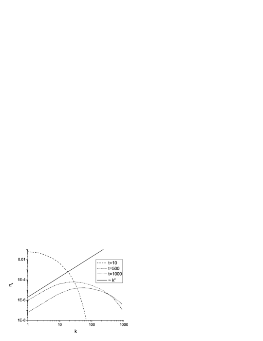
Figure 4: The cluster mass distribution at different time instants for the same system as in Fig. 1. The initial cluster distribution at $t=10$ (long-dashed line) drastically differs from that in the scaling regime, $t\gg 1$. The dotted-dashed and dashed lines show respectively the cluster mass distribution for $t=500$ and $t=1000$. The solid line shows the theoretical prediction, Eq. (17), $n_{k}\sim k^{\mu}$, with $\mu=2\lambda/(1-\lambda)=2$.

Note that the numerical simulations confirm the theoretical form of the steady state cluster mass distribution.

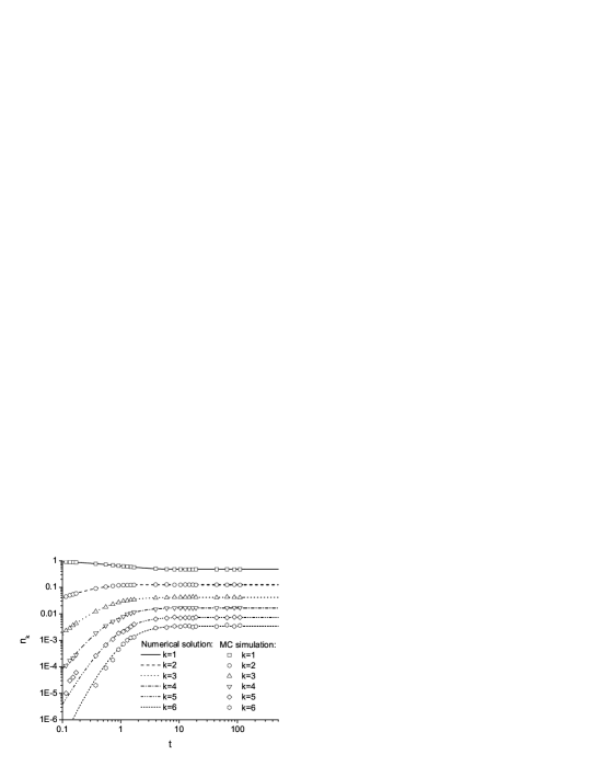
Figure 5: Evolution of cluster concentrations $n_{k}(t)$ for the case of constant kinetic coefficients with $\lambda=2$. After a certain period of time the system relaxes to a steady state. Lines correspond to the numerical solution of 1000 differential equations, symbols – to the results of MC simulation (100 000 monomers) for the monodisperse initial conditions.

Qualitatively similar behavior is observed for the case of the ballistic kinetic coefficients, Eqs. (2), with the constant aggregation and fragmentation energies.

Figure 6: The steady state distribution of cluster mass for the same system as in Fig. 5. The solid line corresponds to the numerical solution, the dotted line – to the theoretical prediction, Eq. (26), $n_{k}=Ak^{-3/2}e^{-\gamma k}$. The constant $\gamma=0.465$, obtained by fitting, is very close to the theoretical value of $\gamma=0.495$, Eq. (29).

Again, for $\lambda<1$, as for constant kinetic coefficients, clusters unlimitedly grow, Fig. 7, while for $\lambda>1$ the system relaxes to a steady state, Fig. 8. The cluster mass distribution in the steady state may be anew very well fitted with the nearly-exponential form, Eq. (26), see Fig. 9.

In Fig. 10 the prediction (35) of the scaling theory is compared with the numerical data. Again we see that the agreement between the theory and simulations is rather satisfactory.

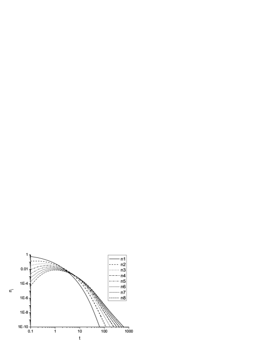
Figure 7: Evolution of cluster concentrations $n_{k}(t)$ for the case of ballistic kinetic coefficients with constant aggregation and fragmentation energies $E_{\rm agg}/T=0.9$, $E_{\rm frag}/T=3$ and $\lambda<1$. The cluster dimension is $D=3$.

Finally Fig. 11 illustrates evolution of the system with the ballistic coefficients that depend on the cluster mass in accordance with Eqs. (36) and (37). It is interesting to note that the system tends initially to a quasi-steady state, as previously for the case of $\lambda>1$, but then a cross-over to a different evolution regime, corresponding to $\lambda<1$ takes place. In the latter regime all cluster concentrations decay with a similar slope, close to $t^{-1}$, still to be explained theoretically.

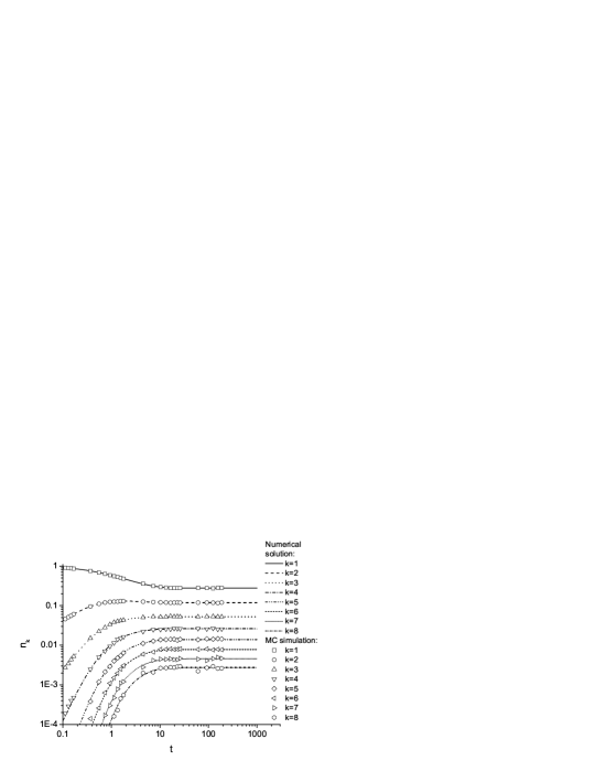
Figure 8: Evolution of cluster concentrations $n_{k}(t)$ in the case of ballistic kinetic coefficients with constant aggregation and fragmentation energies $E_{\rm agg}/T=0.3$, $E_{\rm frag}/T=3$ and $\lambda>1$. The cluster dimension is $D=3$. Similar to the case of constant kinetic coefficients, the system relaxes to a steady state. Lines correspond to the numerical solution of 1000 equations, symbols – to the results of MC simulation (100 000 monomers) for the monodisperse initial conditions.

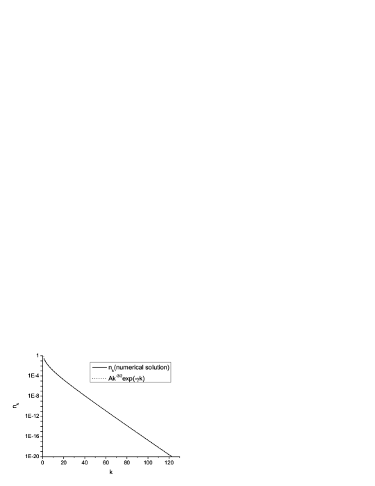
Figure 9: steady state cluster mass distribution of $n_{k}$ for the same system as in Fig. 8. Similar to the case of constant kinetic coefficients with $\lambda>1$, the distribution $n_{k}$ has a nearly-exponential form, Eq. (26), $n_{k}=Ak^{-3/2}e^{-\gamma k}$. The constant $\gamma=0.315$ is obtained by fitting.

Figure 10: Evolution of total number of clusters $N(t)$ for the case of ballistic kinetic coefficients with constant aggregation and fragmentation energies $E_{\rm agg}/T=0.9$, $E_{\rm frag}/T=3$ and $\lambda<1$ for different cluster dimensions $D$. Solid lines correspond to the numerical solution of 1000 differential equations, dotted lines show the prediction of the scaling theory, Eq. (35).

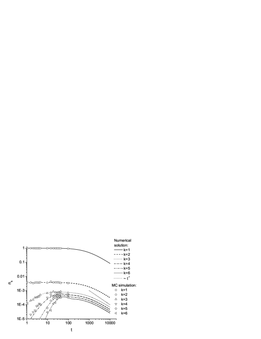
Figure 11: Evolution of the cluster concentrations $n_{k}(t)$ for the case of ballistic coefficients $C_{ij}$, $A_{ij}$ with the mass-dependent aggregation and fragmentation energies $E_{\rm agg}(i,j)$ and $E_{\rm frag}(i,j)$, given by Eqs. (36) and (37) with $E_{\rm agg}^{0}/T=0.1$, $E_{\rm frag}^{0}/T=0.6$. Lines correspond to the numerical solution of 1000 differential equations, symbols – to the results of MC simulation (100 000 monomers) for the monodisperse initial conditions. The cluster dimension is $D=3$. Note that the system tends initially to a steady state, clearly seen for the first few clusters masses. Later its evolution alters to the regime corresponding to the unlimited cluster growth. In this regime the cluster concentrations decay with a slope close to $\sim t^{-1}$, showed in the figure by the dotted line).

5 Conclusion

We analyzed the dynamics of a system where particles move ballistically and undergo collisions which can lead to decrease or increase of the number of particles. The precise outcome depends on the kinetic energy $E_{\rm kin}$ in the center-of-mass reference frame. We proposed a simple model with two threshold energies, $E_{\rm agg}$ and $E_{\rm frag}$, which define a type of an impact: For $E_{\rm kin}<E_{\rm agg}$ the colliding particles merge, for $E_{\rm agg}\,<\,E_{\rm kin}\,<\,E_{\rm frag}$ they rebound, and for $E_{\rm frag}\,<\,E_{\rm kin}$ one the particles (the larger one) splits upon the collision. We assume that the aggregates are composed of $1,2,\ldots,k,\ldots$ monomers and split into two equal (for an even number of monomers in the cluster) or almost equal (for an odd number of monomers) pieces. The monomers are assumed to be stable, that is, they do not further split. For this model we wrote the Boltzmann kinetic equation for the mass-velocity distribution function of the aggregates and derived rate equations for the time evolution of the cluster concentrations. The ballistic rates were obtained in terms of the aggregation and fragmentation energy thresholds $E_{\rm agg}$ and $E_{\rm frag}$, masses of the colliding particles and the temperature of the system (which was assumed to be constant). The Maxwellian velocity distribution for all species in the system was also assumed.

We analyzed theoretically and studied numerically the rate equations. In the numerical studies we used two different methods – the solution of the system of differential equations and Monte Carlo modeling. Both numerical methods yielded very close results. We started with the simplest case of constant rates and observed two opposite evolution regimes — the regime of unlimited cluster growth and of the relaxation to a steady state; we described both these cases analytically. For the regime of the unlimited cluster growth we obtained the asymptotic time dependence for the cluster concentrations and for their mass distribution. For the relaxation regime, which corresponds to the prevailing fragmentation, we derived the asymptotic behavior of the stationary mass distribution. In the evolving regime, the cluster concentrations decay as a power law in time; the stationary mass distribution has a nearly exponential form. Theoretical predictions are in a good agreement with numerical results.

We also studied the case of mass-dependent rates arising in the situation when aggregation and fragmentation energy thresholds are constant. We observed that the behavior of the system is qualitatively similar to that of the system with the constant rates. Surprisingly, we detected that the steady state cluster mass distribution has also a near-exponential form. We developed a scaling theory for the asymptotic large-time behavior of the cluster concentrations and checked it numerically for different fractal dimensions of the aggregates. The numerical data agree well with the results of our theory.

Finally, we explored numerically the case of the ballistic kinetic coefficients with the aggregation and fragmentation energies depending on the mass of colliding particles. For the aggregation energy threshold we use the available in literature result for a collision of particles with surface adhesion. For the fragmentation energy threshold we adopted a model where $E_{\rm frag}$ is proportional to the surface energy of the maximal cross-section of the larger particle in the colliding pair. For this model the dependence on mass of $E_{\rm frag}$ is much stronger than that of $E_{\rm agg}$. As the result, the evolution of the system, where the fragmentation initially prevails and drives it to a steady state, alters at later time when the unlimited cluster growth eventually wins and then it continues ad infinitum.

References

- [1] Chokshi A, Tielens A G G and Hollenbach D 1993 Astrophys. J. 407 806
- [2] Dominik C and Tielens A G G 1997 Astrophys. J . 480 647
- [3] Ossenkopf V 1993 Astron. Astrophys. 280 617
- [4] Spahn F, Albers N, Sremcevic M and Thornton C 2004 Europhys. Lett. 67 545
- [5] Greenberg R, Davis D R, Weidenschilling S J, and Chapman C R 1983 Bull Amer. Asiron. Soc. 15 812
- [6] Weidenschilling S J, Chapman C R, Davis D R and Greenberg R 1984 in In Planetary Rings (R. Greenberg and A. Brahic, Eds.), pp. 367-416
- [7] Longaretti P-Y 1989 Icarus 81 51
- [8] Ben-Naim E, Krapivsky P, Leyvraz F and Redner S 1994 J. Phys. Chem. 98 7284
- [9] Carnevale G F, Pomeau Y and Young W R 1998 Phys. Rev. Lett. 64 2913
- [10] Trizac E and Hansen J-P 1995 Phys. Rev. Lett. 74 4114
- [11] Frachebourg L 1999 Phys. Rev. Lett. 82 1502
- [12] Frachebourg L, Martin Ph A and Piasecki J 2000 Physica 279 69
- [13] Trizac E and Krapivsky P L 2003 Phys. Rev. Lett. 91 218302
- [14] Brilliantov N V and Spahn F 2006 Mathematics and Computers in Simulation 72 93
- [15] Cheng Z and Redner S 1990 J. Phys. A 23 1233
- [16] Krapivsky P and Ben-Naim E 2003 Phys. Rev. E 68 021102
- [17] Pagonabarraga I and Trizac E 2003 in Granular Gas Dynamics Eds. Poeschel T and Brilliantov N (Springer Berlin)
- [18] Hidalgo R C and Pagonabarraga I 2008 Phys. Rev. E 77 061305
- [19] Marsili M and Zhang Yi-C 1996 Phys. Rev. Lett. 77 3577
- [20] Brilliantov N V and Pöschel T 2004 Kinetic theory of Granular Gases (Oxford University Press)
- [21] Garzo V and Dufty J W 1999 Phys. Rev. E 59 5895
- [22] Planetary Rings (Ed. Greenberg R and Brahic A) 1984 (Tucson Az Arizona University Press)
- [23] van Dongen P G J and Ernst M H 1985 Phys. Rev. Lett. 54 1396
- [24] Leyvraz F 2003 Physics Reports 383 95
- [25] Cheng Z and Redner S 1988 Phys. Rev. Lett. 60 2450
- [26] Brilliantov N V, Albers N, Spahn F and Poeschel T 2007 Phys. Rev. E 76 051302
- [27] Gillespie D T 1976 J. Comput. Phys. 22 403
- [28] Feistel R 1977 Wiss. Z. Univ. Rostock 26 663
- [29] Poeschel T, Brilliantov N and Frommel C 2003 Biophysical Journal 85 3460