Scaling and the continuum limit of gluo$N_{c}$ plasmas

Abstract

We investigated the finite temperature ($T$) phase transition for SU($N_{c}$) gauge theory with $N_{c}=4$, 6, 8 and 10 at lattice spacing, $a$, of $1/(6T)$ or less. We checked that these theories have first order transitions at such small $a$. In many cases we were able to find the critical couplings with precision as good as a few parts in $10^{4}$. We also investigated the use of two-loop renormalization group equations in extrapolating the lattice results to the continuum, thus fixing the temperature scale in units of the phase transition temperature, $T_{c}$. We found that when $a\leq 1/(8T_{c})$ the two-loop extrapolation was accurate to about 1–2%. However, we found that trading $T_{c}$ for the QCD scale, $\Lambda_{\overline{\scriptscriptstyle MS}}$, increases uncertainties significantly, to the level of about 5–10%.

I Introduction

Since the realization thooft that a non-trivial and tractable limit is obtained for SU($N_{c}$) gauge theories when the gauge coupling, $g$, is taken to zero and the number of colours, $N_{c}$, is taken to infinity, keeping the combination $g^{2}N_{c}$ fixed, there has been much work on this limit catchall . Most such work sums large classes of Feynman diagrams and therefore is closely related to perturbation theory. The hope is that the limiting theory and a small number of corrections in a series in $1/N_{c}$ would allow us to understand the physically interesting theory with $N_{c}=3$. Lattice calculations are of help in testing this conjecture by making the connection from the other direction— by simulations and complete non-perturbative computations at finite $N_{c}$. They test whether a short series in $1/N_{c}$ for $N_{c}\geq 3$ extrapolates correctly to the tractable limit of $N_{c}\to\infty$. However, in order to test the continuum computations, one must also take the continuum limit of the lattice theories. This is the main thrust of this paper.

The theory with $N_{c}=3$ has been studied extensively before nc3 , and its continuum extrapolation using the renormalized weak coupling expansion has been studied and found to work scaling . We shall have occasion to use these results at various points in this paper. The finite temperature transition has been studied before in 3+1 dimensions on lattices with $a=1/(4T)$ for $N_{c}=4$ nc4 . These early studies found that the crossover from strong to weak coupling, which is a lattice artifact, interfered with the finite temperature transition. Variant actions were invented to solve this problem datta . A modern solution which depends on today’s vastly improved computational power is to just go to larger $N_{t}$ with the simplest action. For larger $N_{c}$ there have been some studies recently with $N_{t}=5$, 6 and 8 nclarger . These earlier works have presented evidence for a first-order thermal phase transition. For $N_{c}=4$, $\Lambda_{\overline{\scriptscriptstyle MS}}$ has been extracted from data on the string tension in the Schrödinger functional scheme ncsf .

In this paper we investigate the continuum limit of the finite temperature deconfinement transition in SU($N_{c}$) pure gauge theory for $N_{c}>3$. The main thrust of our study is to control the approach to the continuum limit by performing simulations of the 3+1 dimensional theories at a succession of lattice spacings, $a$, and then using the weak coupling expansion for the extrapolation to zero lattice spacing. It turns out that with today’s computational power it is quite possible to reach lattice spacings small enough for two-loop renormalization group equations (RGEs) to be useful for the continuum extrapolation. Indeed, at the lattice spacings that we use, even the one-loop flow is a good rough indicator of the continuum limit.

In order to perform these precision tests of the continuum limit we performed lattice simulations of SU(4), SU(6), SU(8) and SU(10) theories. In all cases we simulated theories with lattice cutoffs of $a=1/(6T)$ and $1/(8T)$, and in some cases for even smaller lattice spacings, going down to lattice spacing of $1/(12T)$ in one case. We performed finite size scaling studies, thus extrapolating to the thermodynamic limit of infinite spatial volumes, to check that the thermal phase transitions is actually of first order at lattice spacings $a\leq 1/(6T)$. Coupled with the continuum extrapolations that we discuss next, this verifies earlier arguments about the order of the finite temperature phase transition in continuum theories with $N_{c}\geq 3$ svetitsky .

Through the finite size scaling analysis we located the phase transition point with a statistical precision of a few parts in $10^{4}$. We found that the location of the phase transition point scales as expected in the limit of $N_{c}\to\infty$. With this precision we could test the two-loop RG flow to a statistical accuracy of a few parts in $10^{3}$. It turned out that at lattice spacing of $a\leq 1/(8T_{c})$, the two-loop RGE is trustworthy in extrapolation towards the continuum, within $3\sigma$ of the statistical accuracy. In all this the quantity $T_{c}$ is used to set the scale of measurements.

Any test of a weak coupling expansion involves the choice of an RG scheme, i.e., a choice of a measurement used to define the running coupling in the gauge theory. If the perturbation theory is accurate, and all orders in the expansion are available, then the choice of the scheme is immaterial for any measurement. However, in all practical cases only a small number of terms in the weak coupling expansion are available. We found that for the determination of the temperature scale in terms of $T_{c}$ the scheme dependence is statistically significant, but small in magnitude, being around 1–2%. This indicates that the lattice spacings used in our study are small enough for the use of the weak-coupling expansion. It seems likely that three-loop computations can improve matters.

This could be the first indication that non-perturbative lattice computations for $N_{c}>3$ are at a point where they are more reliable than the perturbative series needed for the continuum extrapolation. Needless to say, one could just push the non-perturbative lattice simulations to smaller and smaller $a$ until the running coupling (at the scale of $a$) decreases significantly and the available perturbative expansions begins to be more accurate. However, it is more cost-effective to develop the perturbation theory to higher order.

In performing a weak coupling expansion the scale of choice is one which defines how fast the coupling changes asymptotically when measured at two different length scales. This intrinsic scale of QCD is called $\Lambda_{\overline{\scriptscriptstyle MS}}$. We found that the determination of $\Lambda_{\overline{\scriptscriptstyle MS}}$ in terms of the non-perturbatively determined scale $T_{c}$ is quite uncertain. While the statistical errors are under control, the scheme dependence is quite large. Our observations seem to indicate that one needs smaller lattice spacings to stabilize the transformation from $T_{c}$ to $\Lambda_{\overline{\scriptscriptstyle MS}}$.

This paper is structured as follows: in the next section we discuss the technicalities of the lattice simulations. Following this we present our results for the finite temperature transition and its extrapolation to the thermodynamic limit. Next, we discuss the continuum limit, the setting of the temperature scale and the extraction of $\Lambda_{\overline{\scriptscriptstyle MS}}$. The final section contains a summary of our results. Some parts of our results have been reported earlier in conference proceedings confs .

II Simulations, measurements and other technicalities

$N_{t}$	$N_{c}=4$	$N_{c}=6$	$N_{c}=8$	$N_{c}=10$
4	12, 16, 18, 20, 24	12, 16, 20
6	16, 18, 20, 22, 24	14, 16, 18, 20, 24	$16^{*}$	$16^{*}$
8	22, 24, 28, 30	20, $24^{*}$	$16^{*}$	$16^{*}$
10	24	$24^{*}$
12	24

Table 1: For each $N_{c}$ and $N_{t}$ the values of $N_{s}$ used in the simulations are given. Runs which are exploratory are marked by asterisks. The remaining runs are meant to yield precision data; for these the details of the statistics are given in Table 6. Zero temperature runs were performed for $N_{s}=N_{t}=16$ for all $N_{c}$ and $N_{s}=N_{t}=24$ for $N_{c}=4$ and 6.

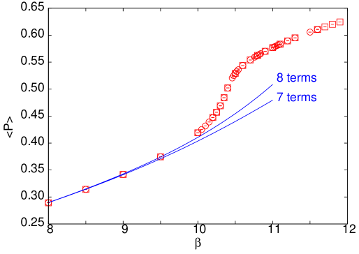
Figure 1: The average plaquette as a function of the bare coupling for $N_{c}=4$ on a $16^{4}$ lattice. Above $\beta=10$ the strong coupling series no longer predicts $\langle P\rangle$ accurately, and the theory crosses over to the weakly coupled phase.

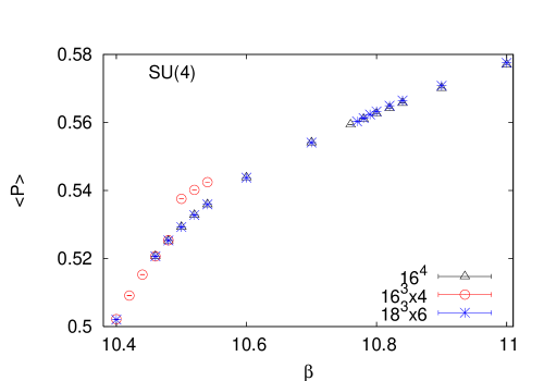
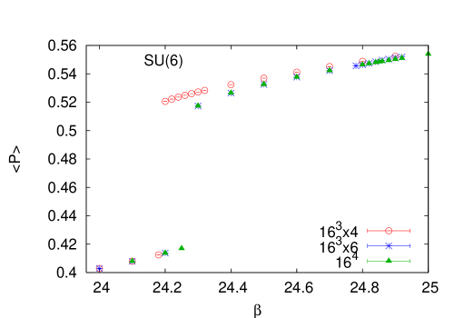
Figure 2: The average plaquette as a function of the bare coupling for $N_{c}=4$ and 6 on various lattice sizes. For SU(4) on a lattice with $N_{t}=4$ there is a jump in $\langle P\rangle$ at $\beta_{c}=10.48$ where the first order thermal phase transition occurs with a jump in $\langle|L|\rangle$. However, at larger $N_{t}$ there is no jump in $\langle P\rangle$. For SU(6) there is a jump in $\langle P\rangle$ at all $N_{t}$. For $N_{t}=4$ the jump occurs at the thermal phase transition, but at all other $N_{t}$ the bulk and thermal transitions are decoupled.

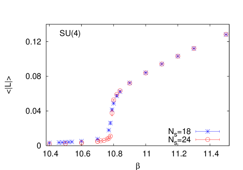
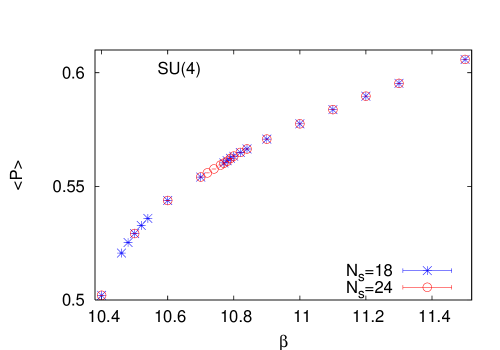
Figure 3: $\langle|L|\rangle$ and $\langle P\rangle$ at functions of $\beta$ on $6\times 18^{3}$ and $6\times 24^{3}$ lattices for SU(4). A rapid change at $\beta_{c}=10.78$ is seen in $\langle|L|\rangle$, whereas $\langle P\rangle$ is continuous. For $N_{t}>4$ the bulk and thermal transitions are decoupled for all $N_{c}$, as shown by this kind of observation.

In this study we use the Wilson action—

$$S=\beta\sum_{i,\mu<\nu}\left[1-{\rm Re}\,P_{\mu\nu}(i)\right],$$ (1)

where $P_{\mu\nu}(i)$ is the trace of the product of SU($N_{c}$) valued link matrices, $U$, around a plaquette, starting from the site $i$ and touching the site $i+\mu+\nu$. The trace is normalized by a factor of $N_{c}$, so that by this definition the trace of an unit matrix is unity. The lattices have size $N_{t}\times N_{s}^{3}$ in units of the lattice spacing, $a$. The physical extent of the lattice is $aN_{t}=1/T$ and $\ell=aN_{s}=\zeta/T$ where $\zeta=N_{s}/N_{t}$ is called the aspect ratio. Increasing $\zeta$ at fixed $T$ corresponds to increasing the volume, $V=\ell^{3}$. The bare gauge coupling is $g^{2}=2N_{c}/\beta$.

The partition function,

$$Z(V,T)=\int{\cal D}U{\rm e}^{-S[U]},$$ (2)

is sampled using a Monte Carlo procedure in which over-relaxation steps are mixed with heat-bath updates. A large fraction of the CPU time is taken up in the computation of the product of matrices connecting to a given matrix (called staples). This computation scales as $N_{c}^{3}$, since the time is dominated by the multiplication of $N_{c}\times N_{c}$ matrices. Therefore, for each computation of a staple, it would make sense to update each of the $N_{c}(N_{c}-1)/2$ SU(2) subgroups of SU($N_{c}$) a fixed number of times algo . When we update all SU(2) subgroups once in every step of a composite sweep which contains three steps of over-relaxation per step of heat-bath, then about 50% of the CPU time is spent in the computation of staples, about 33% in the over-relaxation update, and about 12% in the heat-bath. The rest of the time is spent in the measurement of plaquettes and Polyakov loops. These fractions are almost independent of $N_{c}$, whereas the actual CPU time per link update scales very close to $N_{c}^{3}$. It was argued earlier wolff that in an optimum hybrid over-relaxation algorithm the number of over-relaxation steps should be increased linearly with $N_{s}$. If this were to be done, then relatively less time would be spent in computing staples, resulting in more optimal use of CPU time.

We performed simulations of four theories. An overview of the runs is given in Table 1 and its caption. Almost all zero temperature runs collected statistics of several tens of thousands of composite sweeps, and most runs have statistics of over half a million composite sweeps. The statistics of a set of measurements should actually be judged by the auto-correlation time, $\tau_{int}$, since the error in a measurement, $E$, is related to the variance of the measurements, $\sigma^{2}$, through the formula $E^{2}=\tau_{int}\sigma^{2}/N$ where $N$ is the number of measurements. Auto-correlation functions of the plaquette at $T=0$ show that $\tau_{int}$ varies between approximately 1 and 10 sweeps. Since we study first order phase transitions, $\tau_{int}$ in the transition region for the order parameter, $L$, is closely related to the number of tunnelings between different phases fse . The statistics collected close to the transition region are summarized in Table 6.

SU($N_{c}$) theories with the action in eq. (1) exhibit a bulk transition when $N_{c}$ is large enough. This transition can be monitored in zero temperature simulations using the expectation value of the plaquette, $\langle P\rangle$, where

$$P=\frac{2}{d(d-1)N_{s}^{3}N_{t}}\sum_{i,\mu<\nu}{\rm Re}\,P_{\mu,\nu}(i),$$ (3)

and $d=4$ for our purposes. On the small-$\beta$ side of the transition, one expects the strong coupling series for $\langle P\rangle$ to work; this is an expansion of $\langle P\rangle$ in powers of $\beta^{2}$ drouffe . At larger $\beta$ one expects renormalization group running of $\langle P\rangle$ lepage . For $N_{c}=4$ the change from strong to weak coupling behaviour is fairly smooth, with a cross over in the vicinity of $\beta=10.2$ (see Figure 1). The strong coupling side has little to do with continuum physics. We study thermal physics on the weak-coupling side of this crossover, where, as we show in Section IV, the continuum limit can be taken.

The largest finite volume effect at $T=0$ is expected to occur when the lattice sizes are such that a spurious deconfinement transition takes place saumen . At any given bare coupling $\beta$, there is a critical $N_{*}(\beta)$ such that for $N^{4}$ lattices with $N>N_{*}(\beta)$ one expects small finite size effects. These small effects are expected to scale as $\exp(-\ell m_{0})$ where $m_{0}$ is the mass of the lowest glueball. For SU(3) pure gauge theory, this mass is very high compared to the deconfinement temperature $T_{c}$. If this happens also for $N_{c}>3$, then one expects that finite size effects should be smaller than of order $\exp[-N/N_{*}(\beta)]$. That finite volume effects are indeed small at $T=0$ is borne out by the data in Table 7.

The finite temperature transition was monitored using the order parameter Polyakov loop, $\langle|L|\rangle$, where

$$L=\frac{1}{N_{s}^{3}}\sum_{i}{\rm Tr}\,\prod_{t=1}^{N_{t}}U_{i,\hat{t}},$$ (4)

where the sum over sites, $i$, is restricted to all spatial sites. The order parameter jumps from a zero value at small temperature to a finite value at the thermal transition, signaling deconfinement. The thermal transition is of first order in all the simulations presented here. We found that for SU(4) and SU(6) gauge theories the finite temperature transition and the bulk transition interfere for $N_{t}=4$ (see Figure 2). This is a known phenomenon nc4 ; datta . Since the bulk transition must occur at a fixed lattice spacing, it is natural to expect that by changing $N_{t}$ the bulk and the thermal transitions can be decoupled. It was found nclarger that at larger $N_{t}$ these transitions do separate out (see Figure 3). Therefore, our strategy in this paper is to study larger $N_{t}$, where the thermal transition is in the weak coupling regime, and use these studies to take the continuum limit.

III The deconfinement transition

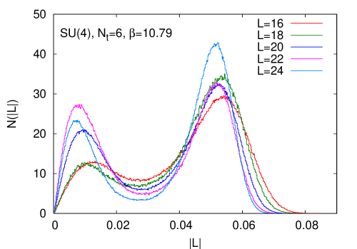
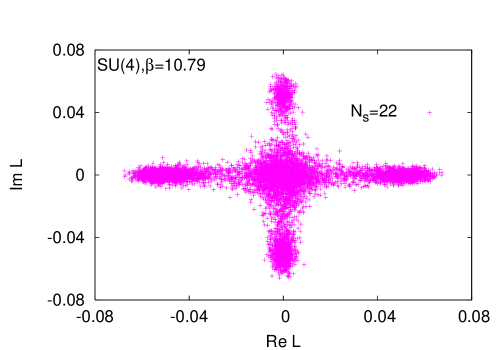
Figure 4: A first order transition, i.e., the coexistence of phases, with different values of $\langle|L|\rangle$, is signaled by a multi-peaked histogram of $|L|$ and the fact that the scatter plot of $L$ in the complex plane shows 5 well developed dense regions— $L=0$ and four complex values of $L$. Here we show these features at a coupling where all five coexisting phases for the SU(4) theory have large weight.

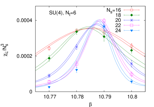
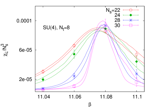
Figure 5: Re-weighting analyses of $\chi_{\scriptscriptstyle L}$ for SU(4) gauge theory shows that on the larger lattices the maximum scales with the lattice volume, $N_{s}^{3}$, indicating a first order phase transition. The analysis is shown for both $N_{t}=6$ and 8.

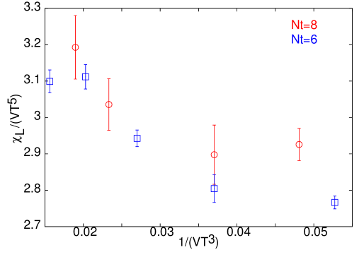
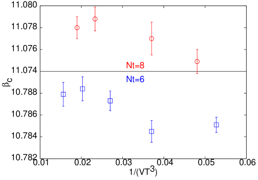
Figure 6: Finite size scaling for SU(4) gauge theory for $N_{t}=6$ (boxes) and 8 (circles). The first panel shows the maximum of $\chi_{\scriptscriptstyle L}/(VT^{5})$ as a function of $1/(VT^{3})$. The second panel shows $\beta_{c}$ as a function of $1/(VT^{3})$. On the largest spatial volumes, the maximum scales as $V$, as expected for a first order phase transition. On the same volumes $\beta_{c}$ reaches a limit which is its thermodynamic value.

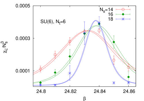
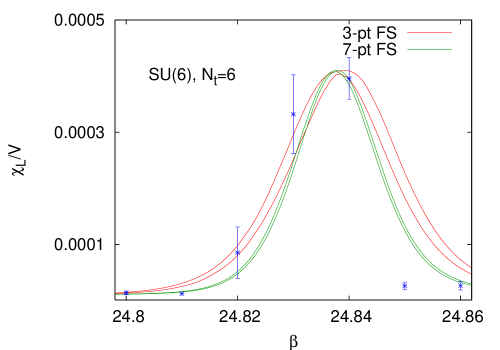
Figure 7: Re-weighting analyses of $\chi_{\scriptscriptstyle L}$ for SU(6) gauge theory shows that on the larger lattices the maximum scales with the lattice volume, $V$, indicating a first order phase transition. Also shown is a multi-histogram analysis on the largest lattice with seven and three input simulations, demonstrating the stability of the estimate of $\beta_{c}$.

The abrupt change of $\langle|L|\rangle$ shown in Figure 3 indicates that the finite temperature transition could be of first order. Clear evidence of the coexistence of phases labeled by the value of $\langle L\rangle$ is obtained from the distribution of $L$. In simulations of the SU(4) theory close to $\beta_{c}$ we found that the system is equally likely to be in the phase with $L=0$ and in four phases with the same $\langle|L|\rangle$ but different phase angles (Figure 4). Hence the histogram of $|L|$ shows two peaks, one close to zero and another elsewhere. A scatter plot of $L$ measured on each gauge field configuration also shows four distinct populations. All these observations are consistent with a first order phase transition. The extraction of the jump in $\langle L\rangle$ at $T_{c}$ needs the renormalized Polyakov loop kay and hence lies beyond the scope of this study.

For more accurate determination of $\beta_{c}$ we defined this coupling by the position of the maximum of the susceptibility of $|L|$—

$$\chi_{\scriptscriptstyle L}=N_{s}^{3}\left\{\left\langle|L|^{2}\right\rangle-\left\langle|L|^{2}\right\rangle\right\}.$$ (5)

For the exploratory runs marked in Table 1, $\beta_{c}$ is estimated from the position of the peak of the values of $\chi_{\scriptscriptstyle L}$ found in a scan over $\beta$, and its quoted error is the spacing in the scan of $\beta$. In all the remaining cases, the objective was precision, and maximum of $\chi_{\scriptscriptstyle L}$ was determined through multi-histogram re-weighting ferrenberg . The errors on $\chi_{\scriptscriptstyle L}$ were defined through a bootstrap procedure combined with the re-weighting. Such analysis requires very large statistics, which is available to us, as shown in Table 6.

A final verification of the order of the transition and the determination of the critical coupling, $\beta_{c}$, require finite size scaling fsep . At a first order transition the maximum value of $\chi_{\scriptscriptstyle L}$ as a function of $\beta$ should scale as $N_{s}^{3}$, i.e.,

$$\chi_{\scriptscriptstyle L}^{m}(N_{s}^{3})=\alpha N_{s}^{3}+\gamma+{\cal O}(N_{s}^{-3}),$$ (6)

when $N_{s}^{3}$ is large enough. Also, the position of the peak, which is our estimate of $\beta_{c}$ at finite volume, should scale as

$$\beta_{c}(N_{s}^{3})=\beta_{c}+\delta N_{s}^{-3}+{\cal O}(N_{s}^{-6}),$$ (7)

as one approaches the thermodynamic limit, $N_{s}\to\infty$. A different definition of $\beta_{c}(N_{s}^{3})$, such as the one where the $N_{c}+1$ different peaks in $L$ have equal weight, could give a different result at finite $N_{s}^{3}$ through a change in $\delta$. Finite volume scalings as in eqs. (6, 7) were observed in SU(3) gauge theory nc3 . The asymptotic region sets in when the lattice size is much larger than the longest correlation length in the system. In this asymptotic region one expects exponentially slow sampling through a standard Monte Carlo procedure, $\tau_{int}\propto\exp(\sigma V^{2/3})$ tauint . As a result, one might expect that as the transition becomes stronger it becomes harder to do a finite size scaling analysis because of an increase in $\sigma$, but the asymptotic finite volume corrections, $\gamma$ and $\delta$, also become relatively smaller.

The variation of $\chi_{\scriptscriptstyle L}$ with $\beta$ obtained through a bootstrap multi-histogram analysis is shown for the SU(4) theory with $N_{t}=6$ and 8 in Figure 5. The position of the peak of $\chi_{\scriptscriptstyle L}$, i.e., $\beta_{c}$, is very stable on the largest lattices used, as shown in Figure 6. It seems that on the two or three largest lattices one enters the region of asymptotic finite size scaling where the formulae in eqs. (6, 7) become applicable. The values of $\beta_{c}$ for $N_{t}=6$ and 8, shown in Table 2, are obtained by fitting eq. (7) with the constraint $\delta=0$ to data on the three largest volumes at each $N_{t}$. If $\delta$ is allowed to vary freely then the best fit changes by at most the quoted error and we find $\delta=-14\pm 14$ for $N_{t}=6$ and $\delta=-32\pm 38$ for $N_{t}=8$.

For the SU(4) theory with $N_{t}=10$ and 12 we have performed simulations on only one lattice volume, as shown in Table 1. While the multi-histogram reweighting analysis allows us to find $\beta_{c}$ at this volume with good precision, an extrapolation to the thermodynamic limit is not yet possible. If we were to assume that $\delta=0$, as in the two smaller $N_{t}$ sets we discussed above, then we can ignore the finite volume shift. However, for $N_{t}=10$ and 12 we use $\zeta$ smaller than the lattices which gave $\delta=0$ for $N_{t}=6$ and 8, so there may be some finite volume shift. To estimate this, albeit crudely, we fitted eq. (7) to our data on the three smallest volumes for $N_{t}=6$ and 8, and extrapolated $\delta$ to $N_{t}=10$ and 12 using a scaling formula for $\delta$ in nclarger . According to this analysis, the thermodynamic limit of $\beta_{c}$ is within twice the error quoted for $N_{t}=10$ and within the quoted errors for $N_{t}=12$.

SU(6) follows the same trend. For all $N_{t}$, one has all the qualitative features of a strong first order phase transition— multiple coexisting phases (6 ordered phases and one disordered in this case) and long auto-correlation times determined by the tunneling rate from one phase to another, growing rapidly with volume. The phase transition is even stronger than SU(4), and a finite size scaling analysis is more delicate.

In Figure 7 we show the multi-histogram reweighting analysis for SU(6). Note that the aspect ratios used in this analysis are smaller than those for SU(4). This is forced on us because the transition is stronger, and therefore $\tau_{int}$ grows faster with $V$. In fact, statistical problems already begin to show up at the largest $V$ for $N_{t}=6$; the run at $\beta=24.85$ has statistically too few tunnelings, since it lies right at the edge of the region of metastability for these lattices. For this system we examined the stability of the analysis through the comparison of the multi-histogram method with seven and three histograms. As shown in Figure 7, the peak is unambiguously determined, since the values of $\chi_{\scriptscriptstyle L}^{m}$ in the two analyses are compatible, as are the estimates of $\beta_{c}$. The reason for the absence of a large systematic error at the peak is that the scan in $\beta$ is fine enough, so that there are enough other histograms to compensate for the one which is improperly sampled.

$N_{c}$	$N_{t}=4$	$N_{t}=6$	$N_{t}=8$	$N_{t}=10$	$N_{t}=12$
3	5.6925 (2)	5.8940 (5)	6.0609 (9)
4		10.788 (1)	11.078 (1)	11.339 (4)	11.552 (17)
6		24.838 (1)	25.470 (3)	26.0 ($1^{*}$)
8		44.7 ($2^{*}$)	45.8 ($2^{*}$)
10		70.5 ($15^{*}$)	73 ($2^{*}$)

Table 2: The critical couplings, $\beta_{c}$, for the first order thermal phase transition for different $N_{c}$ and different temporal lattice sizes, $N_{t}$. Error estimates which are marked by an asterisk are not statistical, as discussed in the text. The results for $N_{c}=3$ were found in nc3 . For $N_{c}>3$ the transition for $N_{t}=4$ falls in the region of the strong to weak coupling cross over, making it hard to distinguish the bulk from the thermal phase transition.

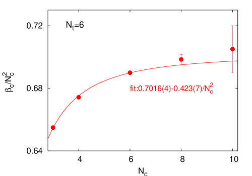
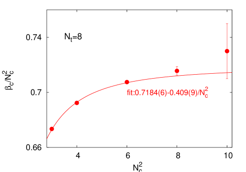
Figure 8: $\beta_{c}$ for different number of colors, on $N_{t}$ = 6 and 8 lattices.

Our simulations of SU(8) and SU(10) pure gauge theory at finite temperature were purely exploratory, being restricted to a single volume at each $N_{t}$. The value of $\beta_{c}$ that we estimate, along with the error bounds given by the scan in $\beta$ are quoted in Table 2.

In Figure 8 we plot these results as a function for $N_{c}$ at fixed lattice spacing $a=1/(N_{t}T_{c})$ for $N_{t}=6$ and 8. We see that a good description of our observations is obtained by a two-term extrapolation to the large-$N_{c}$ limit—

$$\frac{\beta_{c}}{N_{c}^{2}}=\beta_{*}+\frac{\beta^{\prime}_{*}}{N_{c}^{2}}.$$ (8)

The quantity $\beta_{*}$ is expected to increase without bound as $N_{c}\to\infty$. The first correction term, of order $1/N_{c}^{2}$, provides a sufficient description of the data even at $N_{c}=3$. This scaling check shows that for each cutoff, $a=1/(N_{t}T)$ one has a large $N_{c}$ theory which is non-trivial in the limit $g^{2}N_{c}$ fixed, i.e., $\beta/N_{c}^{2}$ fixed.

Note that in the best cases we have achieved accuracies of a few parts in $10^{4}$ in the measurement of $\beta_{c}$. Next we turn to the continuum extrapolation of these measurements and the determination of the temperature scale.

IV Renormalized coupling and the temperature scale

Pure gauge SU($N_{c}$) theory contains a single dimensionless parameter, the coupling, $\alpha_{\scriptscriptstyle S}=g^{2}/4\pi$. Quantum corrections change this into a scale. This can be specified explicitly, as the parameter $\Lambda$, or implicitly, as the value of the running (renormalized) coupling $\alpha_{\scriptscriptstyle S}(\mu)$ at a chosen momentum scale $\mu$. At scales where $\alpha_{\scriptscriptstyle S}$ is small, perturbation theory is expected to work. In that case, changes of the scale of measurements can be accomplished through the use of perturbation theory. In particular, extrapolation of results to the continuum can then be done with ease.

The two-loop RGE can be integrated to trade the running coupling $\alpha_{\scriptscriptstyle S}(\mu)$ for a mass scale,

$$a\Lambda=kR\left(\frac{1}{4\pi\beta_{0}\alpha_{\scriptscriptstyle S}}\right),\qquad{\rm where}\qquad R(x)=\exp(-x/2)x^{\beta_{1}/(2\beta_{0}^{2})},$$ (9)

where $k$ depends on the coupling $\alpha_{\scriptscriptstyle S}$ that enters into these equations. This coupling is measured by some operator dominated by the ultraviolet scale $1/a$. Each such definition of $\alpha_{\scriptscriptstyle S}$ defines an RG scheme. The function $R$ is obtained by integrating the two-loop beta function,

$$\overline{\beta}(g)=\mu\frac{dg}{d\mu}=-\beta_{0}g^{3}-\beta_{1}g^{5},$$ (10)

where $\beta_{0}$ and $\beta_{1}$ are well-known pdg . These coefficients are independent of the scheme. Since $T=1/(aN_{t})$, and we have a determination of $T_{c}$ for different $N_{t}$, by making appropriate lattice measurements of $\alpha_{\scriptscriptstyle S}$ we can measure the temperature scale, $T/T_{c}$. At the same time, one could use eq. (9) to determine the QCD scale $\Lambda_{\overline{\scriptscriptstyle MS}}$ in terms of $T_{c}$.

In order to complete this process, we need to define $\alpha_{\scriptscriptstyle S}$. Two schemes are easily implemented on the lattice. One is the $V$ scheme lepage , in which the potential extracted from Polyakov loop correlations is used to define the renormalized coupling. Equivalently, at two-loop order accuracy, the weak-coupling expansion of the plaquette klassen can be inverted to find $\alpha_{\scriptscriptstyle V}$—

$$-\ln\langle P\rangle=\pi C_{F}\alpha_{\scriptscriptstyle V}(q)\left[1-\frac{11N_{c}}{12\pi}\ln\left(\frac{6.7117}{aq}\right)^{2}\alpha_{\scriptscriptstyle V}(q)\right]$$ (11)

where $C_{F}=(N_{c}^{2}-1)/(2N_{c})$ and $q=k/a$, where $k$ is the same number which is used in eq. (9). In this scheme $k=3.4018$ lepage . Since $\langle P\rangle$ is easily measured and needed for thermodynamic quantities, we prefer to use eq. (11) as a definition of $\alpha_{\scriptscriptstyle V}$ rather than through a separate measurement of the potential. The other definition is the E-scheme, in which the coupling is defined from the plaquette through the formula

$$1-\langle P\rangle=\pi C_{F}\alpha_{\scriptscriptstyle E}(q),$$ (12)

where $q=1/a$, i.e., $k=1$. If the weak coupling expansion were exact, and known to all orders, then there would be no difference between the couplings determined in these two schemes at any cutoff, provided that $\alpha_{\scriptscriptstyle V}$ (or $\alpha_{\scriptscriptstyle E}$) were small enough. Since this is not the case, one must explore RG scheme dependence. A third scheme that we utilize is the $\overline{\rm MS}$ scheme defined through dimensional regularization of the continuum perturbation theory. The known expansion of $\alpha_{\scriptscriptstyle V}$ in terms of $\alpha_{\overline{\scriptscriptstyle MS}}$ peter is used to obtain the latter using the two-loop relation

$$\alpha_{\overline{\scriptscriptstyle MS}}(q^{\prime})=\alpha_{\scriptscriptstyle V}(q)\left[1+\frac{2N_{c}}{3\pi}\alpha_{\scriptscriptstyle V}\right],$$ (13)

where $q^{\prime}=\exp(-5/6)q$ brodsky . In other words, $k=1.4784$ for the $\overline{\rm MS}$ scheme.

The values of the plaquette at zero temperature are measured on the grid of $\beta$ shown in Tables 7 and 8. They are obtained at other points using Lagrange interpolation with polynomials of orders between 1 and 4, and through a cubic spline interpolation. By using such a variety of interpolation schemes we quantify the systematic error in the interpolation at any $\beta$ as the widest dispersion between these schemes. For SU(4) and SU(6) on lattices with $N_{t}\geq 6$, this systematic error is smaller than, or of the same order as, the statistical error in the measurement of the plaquette. For SU(8) and SU(10), the systematic error is larger than the statistical error. These lead to statistical and systematic errors in the determination of the running coupling of the order of a few parts in $10^{5}$. However, when we determine a scale, the largest error is that which comes from the determination of $\beta_{c}$.

A test of the weak coupling expansion for the scale, and the scheme dependence in this is provided by using the determination of $\beta_{c}$ for one $N_{t}$ to predict that at a different $N_{t}$. Since we have measurements for $N_{t}=6$, 8 and 10 for SU(4) and SU(6), we have chosen to examine the temperature predicted by the one-loop and two-loop RGEs for the $N_{t}=6$ and 10 lattices at the $\beta_{c}$ corresponding to the $N_{t}=8$ lattice. This is shown in Table 3. Note that the error of roughly one part in $10^{4}$ in the determination of $\beta_{c}$ translates into an error of about one part in $10^{3}$ in the determination of the temperature scale in the range of temperatures we explore here. Since the accuracy of this error estimate is important in our later reasoning, we performed it by two different methods: first by the usual methods of propagating errors, and then again through a bootstrap analysis. The two errors agreed within 10%, indicating that the estimates are robust. The errors quoted in Table 3 come from the bootstrap analysis.

$N_{c}$	$N_{t}$	Scheme	2-loop	1-loop
4	6	E	1.29709 (167) (7) (1)	1.32333 (184) (8) (1)
		V	1.30782 (174) (8) (1)	1.35339 (204) (9) (2)
		$\overline{\rm MS}$	1.30057 (169) (7) (1)	1.35068 (202) (9) (1)
	10	E	0.80885 (265) (5) (0)	0.79632 (280) (5) (0)
		V	0.80442 (270) (5) (0)	0.78381 (294) (5) (1)
		$\overline{\rm MS}$	0.80757 (267) (5) (1)	0.78517 (292) (5) (0)
6	6	E	1.30504 (165) (10) (3)	1.33190 (181) (11) (4)
		V	1.31675 (172) (10) (4)	1.36476 (200) (12) (4)
		$\overline{\rm MS}$	1.30916 (167) (10) (3)	1.36130 (198) (12) (4)
	10	E	0.81884 (2993) (4) (1)	0.80695 (3161) (4) (1)
		V	0.81435 (3052) (4) (1)	0.79452 (3324) (4) (1)
		$\overline{\rm MS}$	0.81740 (3011) (4) (1)	0.79583 (3307) (4) (1)

Table 3: The values of $T/T_{c}$ at the coupling $\beta_{c}(N_{t}=8)$, for SU($N_{c}$) gauge theory for different $N_{t}$, in different RG schemes, and at different loop orders. The entries give the central value, the statistical error propagated from the uncertainty in $\beta_{c}(N_{t})$, the statistical error from plaquette measurements, and systematic errors from interpolations of plaquette values. For $N_{t}=6$ the exact non-perturbative result is $T/T_{c}=1.33$, and for $N_{t}=10$ it is $T/T_{c}=0.80$.

Some systematics visible in Table 3 is worth explicit comment. The one-loop RG already is close to the exact result, but in all cases performs worse than the two-loop RG. This is expected. Also the RG flow between $\beta_{c}(N_{t}=10)$ and $\beta_{c}(N_{t}=8)$ is better than that between $\beta_{c}(N_{t}=6)$ and $\beta_{c}(N_{t}=8)$. Indeed, for SU(4), where the test is most stringent, the former agrees with the exact non-perturbative result to about $1.5\sigma$ in the V-scheme, and to about 3–4$\sigma$ in the other schemes. The implication is that $N_{t}=8$ is already in a regime where the weak coupling extrapolation to the continuum works, but $N_{t}=6$ may be just a little outside this regime. The scheme dependence is most significant when the two-loop RGE is least reliable, but is less than 1% in all cases.

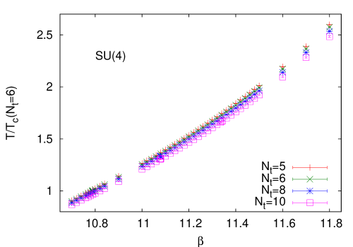
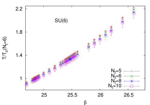
Figure 9: One-loop renormalization group flow for $N_{c}=4$ and 6 in the V-scheme. The data on $\beta_{c}$ for $N_{t}=5$ is taken from nclarger . If the RG were adequate, then the curves for different $N_{t}$ would lie on top of each other. The accuracy of the one-loop flow improves with increasing $N_{t}$.

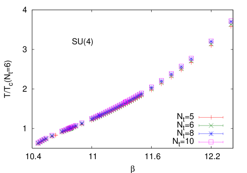
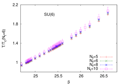
Figure 10: Two-loop renormalization group flow for $N_{c}=4$ and 6 in the V-scheme. The data on $\beta_{c}$ for $N_{t}=5$ is taken from nclarger . Good scaling behaviour is obtained when the curves for different $N_{t}$ lie on top of each other. Excellent scaling is obtained for $N_{t}=8$ and 10.

The one-loop temperature scale is shown in Figure 9 in the V-scheme for a large range of lattice spacings. While this works reasonably well, the improvement in going to two-loops, shown in Figure 10, is obvious. The cutoff effects are small on this scale already for $N_{t}=5$. The two-loop temperature scale in the V-scheme for $N_{t}=6$ and 8, are collected together in Table 9 for future reference. As discussed already, the scale for $N_{t}=8$ is more reliable, and should be used for extrapolations. The scale for $N_{t}=6$ serves to give a rough indication of the kind of systematic errors to be expected: as one can see the difference between these two scales is roughly of 2%.

We have argued here that the continuum extrapolation from $N_{t}=8$ or 10 can be performed using the weak coupling expansion. In weak coupling the reference scale that is used is $\Lambda_{\overline{\scriptscriptstyle MS}}$ and not $T_{c}$. Our analysis above gave us the scales $\Lambda_{E}$ and $\Lambda_{V}$. These can be converted into $\Lambda_{\overline{\scriptscriptstyle MS}}$ alles ; luscher ,

$$\frac{\Lambda_{\overline{\scriptscriptstyle MS}}}{\Lambda_{E}}=\exp\left[\frac{6\pi}{11}\left(1.622268-\frac{\pi}{4N_{c}^{2}}\right)\right],\qquad\qquad\frac{\Lambda_{\overline{\scriptscriptstyle MS}}}{\Lambda_{V}}=\exp\left[-\frac{31}{66}\right].$$ (14)

Using this and the determinations of $\beta_{c}$, we can convert the non-perturbative scale $T_{c}$ into a specification of $\Lambda_{\overline{\scriptscriptstyle MS}}$ in three different schemes.

$N_{c}$	E-scheme		V-scheme		$\overline{\rm MS}$-scheme
	$T_{c}/\Lambda_{\overline{\scriptscriptstyle MS}}$	$c_{2}$	$T_{c}/\Lambda_{\overline{\scriptscriptstyle MS}}$	$c_{2}$	$T_{c}/\Lambda_{\overline{\scriptscriptstyle MS}}$	$c_{2}$
3	1.16 (2)	2.7 (7)	1.11 (2)	1.9 (7)	1.17 (2)	2.5 (7)
4	1.198 (1)	2.49 (5)	1.129 (2)	1.61 (5)	1.203 (2)	2.23 (5)
6	1.193 (1)	1.98 (9)	1.120 (2)	1.05 (9)	1.193 (2)	1.67 (9)

Table 4: Fitted parameters for the non-perturbative beta function in the form of eq. (15). Here $T_{c}/\Lambda_{\overline{\scriptscriptstyle MS}}$ must be considered as a formal fit parameter. Data from all available lattice spacings $1/(12T_{c})\leq a\leq 1/(6T_{c})$ have been used. For $N_{c}=3$ data from $a=1/(4T_{c})$ has also been used.

$N_{c}$	E-scheme	V-scheme	$\overline{\rm MS}$-scheme
3	1.19 (3)	1.12 (3)	1.20 (2)
4	1.235(1)	1.153(1)	1.236(1)
6	1.222(1)	1.135(1)	1.217(1)
8	1.26(6)	1.17(5)	1.25(6)
10	1.48(41)	1.38(39)	1.48(41)
$\infty$	1.22	1.13	1.22

Table 5: $T_{c}/\Lambda_{\overline{\scriptscriptstyle MS}}$ in the continuum limit of SU($N_{c}$) gauge theory for $N_{c}$ = 3,4,6,8, in different schemes using two-loop RGE for $a\leq 1/(8T_{c})$. These values of $T_{c}/\Lambda_{\overline{\scriptscriptstyle MS}}$ are appropriate for use in a two-loop computation.

The test of two-loop RGE in Table 3 showed that this was fairly accurate already at the lattice spacing corresponding to $\beta_{c}$ for $N_{t}=8$ and 10. Therefore it is no surprise that to the same degree of accuracy the ratio $T_{c}/\Lambda_{\overline{\scriptscriptstyle MS}}$ is constant when evaluated at $N_{t}\geq 8$. However, the scheme dependence is much larger for $\Lambda_{\overline{\scriptscriptstyle MS}}$ than for the temperature scale. This happens because the renormalized coupling is not small enough for the eqns. (14) to hold. One could correct these formulae by explicitly including two-loop or higher order correction terms. However, then the ratio $T_{c}/\Lambda_{\overline{\scriptscriptstyle MS}}$ would depend on the scale $a$. This can be avoided only when $\alpha_{\scriptscriptstyle S}$ becomes substantially smaller. However, since $\alpha_{\scriptscriptstyle S}$ runs logarithmically with $a$, that would imply that one has to use lattice spacings which are about 10 times smaller. This is currently outside the reach of our computational abilities.

For SU(3) the range of accuracy of the RGE can be extended by including into it corrections of order $a^{2}$ ehk . This seems to be possible for $N_{c}>3$ too. When we compare $T_{c}/\Lambda_{\overline{\scriptscriptstyle MS}}$ extracted for all $N_{t}$, it seems possible to fit this to a simple $a^{2}$ variation. In principle this term can be used to add an ${\cal O}(a^{2})$ correction to the two-loop beta function by changing $R(x)$ in eq. (9) to $R(x)[1+\eta/N_{t}^{2}]$. We evaluate these corrections by a fit to the lattice spacing dependence of $T_{c}/\Lambda_{\overline{\scriptscriptstyle MS}}$ which renders this ratio flat in the whole range $1/(10T_{c})\leq a\leq 1/(5T_{c})$, i.e., we choose the fit form

$$\frac{T_{c}}{\Lambda_{\overline{\scriptscriptstyle MS}}}|_{N_{t}}=\frac{T_{c}}{\Lambda_{\overline{\scriptscriptstyle MS}}}+\frac{\eta}{N_{t}^{2}}.$$ (15)

Statistically significant results can only be obtained for $N_{c}\leq 6$. Our results for the fit are given in Table 4. One can compare these with the estimate $T_{c}/\Lambda_{\overline{\scriptscriptstyle MS}}=1.187\pm 0.009$ obtained by combining estimates of $T_{c}/\sqrt{\sigma}$ (where $\sigma$ is the string tension) and $\sqrt{\sigma}/\Lambda_{\overline{\scriptscriptstyle MS}}$ reported in nclarger ; allton . The estimation of $\sqrt{\sigma}/\Lambda_{\overline{\scriptscriptstyle MS}}$ removes ${\cal O}(a^{2})$ corrections, as we do here. We note that such a term sums many different types of corrections and amounts to a phenomenological fit of the beta function, i.e., gives what is called the non-perturbative beta-function. For this reason it cannot be regarded as a test of scaling.

The continuum values for $T_{c}/\Lambda_{\overline{\scriptscriptstyle MS}}$, obtained assuming that this ratio is constant for lattice cutoffs $a\leq 1/(8T_{c})$ are collected in Table 5. Note that there are large and statistically significant differences between these results and those in Table 4. Since the latter results constitute a check of two-loop RGE, and the best possible extraction of $\Lambda_{\overline{\scriptscriptstyle MS}}$, they are to be preferred for this purpose. For SU(3) we have performed a re-analysis of the data which was used in scaling without the ${\cal O}(a^{2})$ terms from ehk . This makes the analysis uniform for all $N_{c}$. Note that the dependence on $N_{c}$ is weak. We have added indicative values of this ratio extrapolated to the limit $N_{c}\to\infty$. Since a statistical analysis is not possible, we have not added error bars to this extrapolation. Note that the strong scheme dependence, which we discussed before, propagates to the $N_{c}\to\infty$ limit.

In summary, the two-loop renormalization group equations work well for $a\leq 1/(8T_{c})$, i.e., at the level of 1–2%. Since the largest part of this uncertainty stems from the RG scheme dependence, higher order corrections in the perturbation series for the plaquette could easily improve this description. However, trading the non-perturbative scale $T_{c}$ for the perturbatively determined scale $\Lambda_{\overline{\scriptscriptstyle MS}}$ is not yet possible to better than 5–10%. Improving this would require using lattice spacings which are beyond reach today.

V Conclusions

In this paper we studied the finite temperature phase transition in SU(4), SU(6), SU(8) and SU(10) pure gauge theories at several lattice spacings and extrapolated the results to the continuum. In all these theories at large lattice spacing, $a\simeq 1/(4T_{c})$, a lattice artifact called the bulk phase transition prevents a simple study of finite temperature physics. The order parameter of the bulk transition is the plaquette average, $\langle P\rangle$, whereas that of the finite temperature transition is the Polyakov loop expectation value, $\langle|L|\rangle$. The bulk transition is expected to occur at a (approximately) fixed lattice spacing. We studied these theories at smaller lattice spacings, $a\leq 1/(6T_{c})$, and found that in all cases the finite temperature phase transition can be studied without any interference from the bulk transition (see Figure 3, for example). More details are reported in Section II.

We found a first order finite temperature transition for all these theories. This was established not only by clear signals of multiple coexisting phases labeled by different values of $\langle|L|\rangle$, but, in several cases, also by finite size scaling tests. These studies and also multi-histogram reweighting at fixed volumes allowed us to locate the phase transition with precision which was in many cases as good as a few parts in $10^{4}$. Our results on the finite temperature phase transition are given in Section III, and the locations of the phase transition are collected together in Table 2.

We investigated the continuum extrapolation of our lattice results and found that when the lattice spacing is $a\leq 1/(8T_{c})$ then the two-loop RGE can be used to take the continuum limit. In order to do this one has to use a definition of the renormalized (running) coupling, called an RG scheme. We found that when the location of the phase transition at one lattice spacing is used to predict that at another, then the dependence on the RG scheme is small (see Table 3): the statistical precision is about one part in $10^{3}$, but the scheme dependence is about 2%. This allows us to construct a temperature scale with this degree of precision using the non-perturbatively obtained mass scale, $T_{c}$. Since the scheme dependence is the largest part of the uncertainty, higher order corrections will reduce this error. This is the first instance of a large $N_{c}$ lattice calculation which has reached precisions good enough to test the state of the art in the weak coupling expansion. Details of these tests can be found in Section IV. One useful result is the determination of the temperature scale in SU(4) and SU(6) gauge theories (Table 9).

We tried to use two-loop perturbation theory to trade the scale $T_{c}$ for the scale $\Lambda_{\overline{\scriptscriptstyle MS}}$ which is more commonly used in weak coupling expansions, and found that the scheme dependence becomes significantly more pronounced. The extraction of $\Lambda_{\overline{\scriptscriptstyle MS}}$ by this means gave statistical errors comparable to the temperature scale, but RG scheme dependence of about 10%. A large scheme dependence in trading a non-perturbative scale such as $T_{c}$ for the perturbative scale $\Lambda_{\overline{\scriptscriptstyle MS}}$ is bound to persist in all foreseeable lattice computations.

We found that two results can be easily extrapolated to the limit $N_{c}\to\infty$. The location of the critical point at fixed lattice spacing $a=1/(N_{t}T_{c})$ goes as $\beta_{*}+{\cal O}(1/N_{c}^{2})$ for $N_{c}\geq 3$ (see Figure 8). For $T_{c}/\Lambda_{\overline{\scriptscriptstyle MS}}$ the series could be shorter; we find no statistically significant dependence of $T_{c}/\Lambda_{\overline{\scriptscriptstyle MS}}$ on $N_{c}$ in any of the three RG schemes that we studied (see Table 5).

These computations were carried out on the CRAY-X1 of the ILGTI in TIFR, and on the workstation farm of the Department of Theoretical Physics, TIFR. We would like to thank Ajay Salve for technical support.

Appendix A Some details

Some details of the simulations and detailed tables of some of our results are collected in this appendix.

	$N_{c}=4$						$N_{c}=6$
	$N_{t}=6$			$N_{t}=8$			$N_{t}=6$			$N_{t}=8$
$N_{s}$	$\beta$	Statistics	$\tau_{\rm int}$	$\beta$	Statistics	$\tau_{\rm int}$	$\beta$	Statistics	$\tau_{\rm int}$	$\beta$	Statistics	$\tau_{\rm int}$
14							24.80	2.14	7354
							24.81	1.94	9391
							24.82	2.05	10538
							24.83	1.94	12349
							24.84	1.94	12113
							24.85	2.05	9428
							24.86	2.01	7747
16	10.77	1.56	2367				24.80	2.26	4388
	10.78	4.5	3188				24.81	3.88	12602
	10.79	1.56	3780				24.82	2.29	14827
	10.80	2.6	2566				24.83	2.74	15582
							24.84	2.34	16984
							24.85	4.24	15854
							24.86	0.89	7907
18	10.77	0.92	3263				24.80	3.75	2486
	10.78	0.88	6944				24.81	3.69	315
	10.79	0.88	5944				24.82	3.62	15585
	10.80	1.8	4564				24.83	3.68	18409
							24.84	4.23	18376
							24.85	3.62	3861
							24.86	2.70	4175
20	10.77	2.8	2850							25.42	1.46	5533
	10.78	2.9	6445							25.44	0.90	11482
	10.79	2.8	8192							25.46	0.64	15773
	10.80	4.4	5806							25.48	2.31	15951
										25.50	1.44	15117
22	10.77	2.1	3621	11.06	3.1	5472
	10.78	2.1	6737	11.08	2.9	7019
	10.79	2.1	10700
	10.80	3.4	5256
24	10.77	0.12	1452	11.06	1.08	5959
	10.78	2.9	9063	11.08	1.1	9821
	10.79	2.8	13614
	10.80	2.8	4475
28				11.06	1.5	6753
				11.08	1.4	11935
30				11.06	1.2	2308
				11.08	1.2	15251

Table 6: The statistics (in millions of composite sweeps) used in the re-weighting analysis for $\beta_{c}$ in SU($N_{c}$) gauge theory. Also quoted is the integrated auto-correlation time. Studies at $N_{t}=10$ and 12 have been carried out with statistics of $4\times 10^{5}$ composite sweeps, where $\tau_{int}$ varied between 500 and 1000 sweeps.

SU(4)				SU(6)
$\beta$	$\langle P\rangle$			$\beta$	$\langle P\rangle$
	$N_{s}=16$	$N_{s}=18$	$N_{s}=24$		$N_{s}=16$	$N_{s}=20$	$N_{s}=24$
10.40	0.502033(46)	0.501991(29)	0.502136(18)	24.60	0.537686(30)
10.46	0.520680(25)	0.520728(23)	0.520673(16)	24.70	0.542241(24)
10.48	0.525249(12)	0.525254(16)	0.525259(7)	24.80	0.546406(9)
10.50	0.529260(25)	0.529268(17)	0.529274(15)	24.82	0.547189(10)
10.52	0.532786(15)	0.532749(20)	0.532773(11)	24.84	0.547981(6)
10.54	0.535885(9)	0.535903(16)	0.535903(12)	24.86	0.548764(9)
10.60	0.543796(10)	0.543778(12)	0.543790(7)	24.88	0.549532(8)
10.70	0.554088(7)	0.554097(10)	0.554092(4)	24.90	0.550292(7)
10.76	0.559352(8)		0.559341(5)	24.92	0.551042(6)
10.78	0.561000(4)	0.561005(10)	0.561000(5)	25.00	0.553961(3)
10.79		0.561805(8)	0.561799(4)	25.10	0.557459(5)
10.80	0.562606(7)	0.562605(5)	0.562602(3)	25.20	0.560805(4)
10.82	0.564167(7)	0.564166(8)	0.564169(4)	25.30	0.564026(4)	0.564012(4)	0.564015(3)
10.84	0.565700(8)	0.565689(5)	0.565702(3)	25.40	0.567126(4)	0.567119(2)	0.567120(3)
10.90	0.570122(5)	0.570123(4)	0.570120(3)	25.42		0.567727(3)	0.567727(2)
11.00	0.576972(5)	0.576979(5)	0.576984(3)	25.44		0.568332(3)	0.568329(3)
11.02	0.578291(5)		0.578286(4)	25.46		0.568933(3)	0.568931(3)
11.04	0.579577(4)		0.579580(3)	25.48		0.569522(3)	0.569527(3)
11.06	0.580859(5)		0.580851(4)	25.50	0.570130(5)	0.570123(4)	0.570119(3)
11.08	0.582117(5)		0.582109(4)	25.52		0.570709(3)	0.570708(2)
11.10	0.583361(5)	0.583369(3)	0.583363(3)	25.54		0.571293(4)	0.571294(2)
11.20	0.589361(4)	0.589357(3)	0.589360(2)	25.56		0.571880(3)	0.571877(3)
11.30	0.595051(3)	0.595043(4)	0.595051(2)	25.60	0.573043(3)	0.573031(3)	0.573031(2)
11.50	0.605665(5)	0.605652(4)	0.605650(2)	25.70	0.575876(4)
11.60	0.610655(6)	0.610643(4)	0.610630(3)	25.80	0.578631(3)	0.578620(3)	0.578616(3)
				25.90	0.581321(4)
				26.00	0.583937(5)	0.583925(4)	0.583921(4)
				26.10	0.586506(6)	0.586487(3)	0.586485(3)

Table 7: Plaquette expectation values for SU(4) and SU(6). The numbers in brackets denote errors on the least significant digits. Note that the volume dependence is negliglible.

SU(8)		SU(10)
$\beta$	$\langle P\rangle$	$\beta$	$\langle P\rangle$
44.50	0.542133(9)	68.00	0.376818(6)
44.80	0.548772(6)	70.00	0.542542(8)
45.00	0.552860(7)	71.00	0.554874(8)
45.20	0.556747(5)	72.00	0.567207(8)
45.50	0.562252(4)	74.00	0.586693(5)
46.00	0.570739(4)	76.00	0.603381(7)

Table 8: Plaquette expectation values for SU(8) and SU(10), measured on $16^{4}$ lattices. The numbers in brackets are errors on the least significant digit.

SU(4)			SU(6)
$\beta$	$N_{t}=6$	$N_{t}=8$	$\beta$	$N_{t}=6$	$N_{t}=8$
10.70	0.9106(9)	0.6963(6)	24.60	0.8841(4)	0.6714(8)
10.72	0.9311(9)	0.7119(6)	24.70	0.9335(5)	0.7089(9)
10.74	0.9513(10)	0.7274(6)	24.80	0.9818(5)	0.7456(9)
10.76	0.9716(10)	0.7429(6)	24.82	0.9913(5)	0.7529(9)
10.77	0.9817(10)	0.7507(7)	24.84	1.0010(5)	0.7602(9)
10.78	0.9920(10)	0.7585(7)	24.85	1.0059(5)	0.7640(9)
10.79	1.0020(10)	0.7662(7)	24.86	1.0107(5)	0.7675(9)
10.80	1.0122(10)	0.7740(7)	24.88	1.0204(5)	0.7749(9)
10.82	1.0326(10)	0.7895(7)	24.90	1.0301(5)	0.7823(9)
10.84	1.0530(11)	0.8052(7)	24.92	1.0397(5)	0.7896(10)
10.90	1.1151(11)	0.8526(7)	25.00	1.0786(5)	0.8191(10)
11.00	1.2215(12)	0.9340(8)	25.10	1.1277(6)	0.8564(10)
11.02	1.2433(13)	0.9506(8)	25.20	1.1775(6)	0.8943(11)
11.04	1.2654(13)	0.9675(8)	25.30	1.2282(6)	0.9327(11)
11.06	1.2876(13)	0.9845(9)	25.34	1.2487(6)	0.9483(11)
11.08	1.3101(13)	1.0017(9)	25.38	1.2695(6)	0.9641(12)
11.10	1.3331(13)	1.0193(9)	25.40	1.2799(6)	0.9720(12)
11.12	1.3559(14)	1.0368(9)	25.42	1.2904(6)	0.9800(12)
11.14	1.3791(14)	1.0545(9)	25.44	1.3008(6)	0.9879(12)
11.16	1.4028(14)	1.0726(9)	25.46	1.3114(7)	0.9960(12)
11.18	1.4265(14)	1.0908(10)	25.48	1.3221(7)	1.0040(12)
11.20	1.4507(15)	1.1092(10)	25.50	1.3327(7)	1.0121(12)
11.22	1.4748(15)	1.1276(10)	25.52	1.3434(7)	1.0202(12)
11.24	1.4996(15)	1.1466(10)	25.54	1.3542(7)	1.0284(12)
11.26	1.5243(15)	1.1655(10)	25.56	1.3650(7)	1.0366(13)
11.28	1.5496(16)	1.1849(10)	25.60	1.3868(7)	1.0532(13)
11.30	1.5755(16)	1.2046(10)	25.80	1.4989(7)	1.1383(14)
11.32	1.6010(16)	1.2242(11)	25.90	1.5573(8)	1.1827(14)
11.34	1.6271(16)	1.2441(11)	26.00	1.6169(8)	1.2280(15)
11.36	1.6537(17)	1.2645(11)	26.20	1.7415(9)	1.3226(16)
11.38	1.6804(17)	1.2849(11)	26.40	1.8727(9)	1.4222(17)
11.40	1.7077(17)	1.3058(11)	26.60	2.0119(10)	1.5279(18)
11.42	1.7351(17)	1.3267(12)	27.00	2.3149(11)	1.7581(21)
11.44	1.7629(18)	1.3479(12)	27.50	2.7474(14)	2.0865(25)
11.46	1.7911(18)	1.3696(12)
11.48	1.8197(18)	1.3914(12)
11.50	1.8486(19)	1.4135(12)
11.60	1.9988(20)	1.5283(13)
11.70	2.1590(22)	1.6508(14)
11.80	2.3300(23)	1.7816(15)
11.90	2.5126(25)	1.9212(17)
12.00	2.7076(27)	2.0703(18)
12.20	3.1390(32)	2.4001(21)
12.40	3.6320(37)	2.7771(24)

Table 9: $T/T_{c}$ scales for SU(4) and SU(6) gauge theories in the V-scheme, for $N_{t}=6$ and 8. The errors are dominated by the uncertainty in the determination of $\beta_{c}$.

References

- (1) G. ’tHooft, Nucl. Phys., B 72 (1974) 461.
-
(2)
See, for example,
E. Brezin, C. Itzykson, G. Parisi and J.-B. Zuber,
Comm. Math. Phys., 59 (1978) 35;
E. Witten, Nucl. Phys., B 156 (1979) 269;
T. Eguchi and H. Kawai, Phys. Rev. Lett., 48 (1982) 1063;
S. Coleman, in Aspects of Symmetry, Cambridge University Press, 1985, Cambridge, UK;
E. Brezin and S. Wadia, The large N expansion in quantum field theory and statistical physics, World Scientific, 1993, Singapore;
M. J. Teper, Phys. Rev., D 59 (1998) 014512. -
(3)
Y. Iwasaki et al., Phys. Rev. Lett., 67 (1991) 3343;
G. Boyd et al., Nucl. Phys., B 469 (1996) 419. - (4) S. Gupta, Phys. Rev., D 64 (2001) 034507.
-
(5)
A. Gocksch and M. Okawa, Phys. Rev. Lett., 52 (1984) 1751;
G. G. Batrouni and B. Svetitsky, Phys. Rev. Lett., 52 (1984) 2205;
M. Wingate and S. Ohta, Phys. Rev., D 63 (2001) 094502;
R. V. Gavai, Nucl. Phys., B 633 (2002) 127. - (6) S. Datta and R. V. Gavai, Phys. Rev., D 62 (2000) 054512.
-
(7)
B. Lucini, M. Teper and U. Wenger, Phys. Lett., B 545 (2002) 197;
B. Lucini, M. Teper and U. Wenger, J. H. E. P., 0401 (2004) 061;
B. Lucini and M. Teper, J. H. E. P., 0502 (2005) 033. - (8) B. Lucini and G. Moraitis, Phys. Lett., B 668 (2008) 226.
-
(9)
B. Svetitsky and L. G. Yaffe, Nucl. Phys., B 210 (1982) 423;
B. Svetitsky, Phys. Rep., 132 (1986) 1. - (10) S. Datta and S. Gupta, arXiv:0906.3929.
- (11) Ph. de Forcrand and O. Jahn, e-print hep-lat/0503041.
- (12) U. Wolff, Phys. Lett., B 288 (1992) 166.
- (13) A. Billoire et al., Nucl. Phys., B 358 (1991) 231.
- (14) J. M. Drouffe and K. J. M. Moriarty, Phys. Lett., 108 B (1982) 333.
- (15) G. P. Lepage and P. B. Mackenzie, Phys. Rev., D 48 (1993) 2250.
- (16) S. Datta and S. Gupta, Phys. Lett., B 471 (2000) 382.
- (17) S. Gupta, K. Hu
- (18) A. M. Ferrenberg and R. H. Swendsen, Phys. Rev. Lett., 63 (1989) 1195.
-
(19)
C. Borgs and R. Kotecky, Phys. Rev. Lett., 68 (1992) 1734;
S. Gupta, A. Irbäck, M. Ohlsson, Nucl. Phys., B 409 (1993) 663;
A. Billoire, Nucl. Phys. Proc. Suppl., 42 (1995) 21. - (20) S. Gupta, Phys. Lett., B 325 (1994) 418.
- (21) B. A. Berg, Int. J. Mod. Phys., C 3 (1992) 1083.
- (22) C. Amsler et al., Phys. Lett., B 667 (2008) 1.
- (23) T. R. Klassen, Phys. Rev., D 51 (1995) 5130.
- (24) M. Peter, Nucl. Phys., B 501 (1997) 471.
- (25) S. J. Brodksy, G. P. Lepage and P. B. Mackenzie, Phys. Rev., D 28 (1983) 228.
- (26) B. Alles, A. Feo and H. Panagopoulos, Nucl. Phys., B 491 (1997) 498.
- (27) M. Luscher and P. Weisz, Nucl. Phys., B 452 (1995) 234.
-
(28)
C. Allton, hep-lat/9610016;
R. G. Edwards, U. Heller, T. Klassen, Nucl. Phys., B 517 (1998) 377. - (29) C. Allton, M. Teper and A. Trivini, J. H. E. P., 0807 (2008) 021.