Quantum Coherence of Discrete Kink Solitons in Ion Traps

Abstract

We propose to realize quantized discrete kinks with cold trapped ions. We show that long-lived solitonlike configurations are manifested as deformations of the zigzag structure in the linear Paul trap, and are topologically protected in a circular trap with an odd number of ions. We study the quantum-mechanical time evolution of a high-frequency, gap separated internal mode of a static kink and find long coherence times when the system is cooled to the Doppler limit. The spectral properties of the internal modes make them ideally suited for manipulation using current technology. This suggests that ion traps can be used to test quantum-mechanical effects with solitons and explore ideas for the utilization of the solitonic internal-modes as carriers of quantum information.

Solitons are localized configurations of nonlinear systems which are nonperturbative and topologically protected [1]. Quantum-mechanical properties of solitons, such as squeezing, have been predicted and measured in optical systems [2]. Quantum dynamics has been observed with a single Josephson junction soliton [3]. In waveguide arrays [4, 5] and Bose-Einstein condensates [6] solitons are mean field solutions, localized to a few sites of a periodic potential. In chains of coupled particles, solitons are discrete spatial configurations, as in the Frenkel-Kontorova (FK) model [7, 8].

Discrete solitons of the FK model and its generalizations are referred to as kinks. An important property of kinks is the existence of localized modes. One mode is the kink’s translational ‘zero-mode’, whose frequency generally rises above zero. Other localized modes are known as ‘internal modes’ [9, 10]. Physically they describe ‘shape-change’ excitations of the kink and typically they are separated by an energy gap from other long-wavelength phononic modes. It was suggested to use the internal mode as a carrier of quantum information [11].

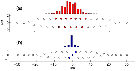
Figure 1: Metastable linear trap configurations with 33 ions. (a) An extended kink. The localized internal mode (red bars) involves $\sim{10}$ ions. (b) A highly discrete ’odd’ kink. A localized internal oscillation (blue bars) involves $\sim 3$ ions.

Quantum information processing in ion traps [12] has dramatically improved over the last decades [13, 14]. Recently there has been a considerable interest in using trapped ions for quantum simulation of various systems such as spin-chains [15, 16, 17] and Bose-Hubbard models [18], field models [19], cosmological effects [20] and black holes [21]. It was suggested to realize a 1D generalization of the FK model by adding an external periodic potential to an ion trap [22].

In this Letter we demonstrate that quantum coherence in static discrete kinks can be observed with ordinary Paul traps without external additions. We explore quasi-2D discrete kinks resembling those of the zigzag model [23]. In the linear trap we find local metastable deformations of the zigzag structure [24], as depicted in Fig. 1, which are long-lived already with a moderate number of ions, $N\gtrsim 20$. In a circular trap with an odd number of ions, similar configurations form the ground state. We study the robustness of a high-frequency internal mode of the kink against decoherence in the thermal environment of all the other modes. With all nonlinear interactions accounted for, we numerically integrate a non-Markovian master equation, which leads us to our main result: already at the standard Doppler cooling limit coherence persists in the internal mode for many oscillations. This could allow a first direct measurement of decoherence time of solitons.

Let us consider $N$ ions trapped either in a linear trap or in a circular ring trap. Throughout this Letter we use nondimensional units by employing the natural length scale $d=\left(e^{2}/m\nu^{2}\right)^{1/3}$ and time scale $1/\nu$, where $m$ is the ions’ mass and $\nu$ is the axial (radial) trapping frequency in the linear (circular) trap. In the linear case the trapping potential can be expressed as $V=\sum_{i}^{N}\frac{1}{2}\left(x_{i}^{2}+\beta y_{i}^{2}\right)$. At sufficiently high transverse trapping $\beta$, the ions crystalize in a one-dimensional chain along the $x$-axis. When $\beta$ is lowered, the ions undergo a second order phase transition [25] and the lowest energy state has a zigzag shape with interesting quantum mechanical properties [26]. However, depending on $\beta$, other metastable configurations exist. We have identified two additional types of configuration that are not destroyed by thermal fluctuations at up to $\sim 15$ times the Doppler temperature. Figure 1(a) shows an extended soliton-like deformation ($\beta=40$), with a cross-over of the upper ions of the zigzag above the lower ones. In Fig 1(b) one ion is forced out of the zigzag to form a dense defect at the center ($\beta=85$).

In the ring trap, ions are confined at uniform density around a circle and the radial confining potential is

$$V=\sum_{i}^{N}{\frac{1}{2}\left(\left\|\vec{R}_{i}\right\|-\gamma\frac{N}{2\pi}\right)^{2}},$$ (1)

where $\vec{R}_{i}\equiv\left(x_{i},y_{i}\right)$ and $\gamma$ measures the strength of the radial trapping, independently of the number of ions. $\gamma\propto\nu^{2/3}$ is varied by changing the radial trapping frequency. The lowest energy configuration with an odd number of ions can be one of a few types. At high $\gamma$, close to the phase-transition from a 1D chain ($\gamma\approx 1.6$), the kink is localized with two ions facing inside the zigzag shape. At lower values of $\gamma$ the two kink-core ions lie outside of the zigzag, as shown in Fig. 2, lower inset. When lowering $\gamma$ further, an extended kink is formed (Fig. 2, upper inset). The ring topology protects kinks in this trap from breaking.

In the absence of a kink the linearized frequency spectrum of the normal-modes consists of a phonon band terminated at a cutoff frequency that depends on the ion density. The presence of the kink causes a few highly localized modes to split away from the rest of the spectrum. In a large range of values for the trap parameter, there exists a localized mode lying above the band and separated by a gap (Figs. 2, 4(a)). This mode corresponds to out-of-phase oscillations of the ions in the kink’s core. It is this ”high-frequency mode” which we suggest for coherent manipulations.

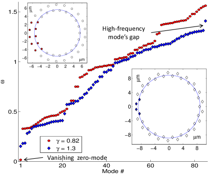
Figure 2: Dispersion-relations in the circular trap. At $\gamma=0.82$ (red circles and upper inset) the kink is extended, there is no gap at the top of the spectrum and the translational mode’s frequency approaches zero. At $\gamma=1.3$ (blue diamonds and lower inset) the kink is localized on 4 ions and the localized modes at the top and bottom of the spectrum are gap-separated. The mode corresponding to rotational symmetry of the entire trap has been omitted.

Expanding the Hamiltonian in a perturbative series about the classical kink configuration, $\vec{R}_{i}=\vec{R}^{0}_{i}+\delta\vec{R}_{i}$, we switch variables to the normal coordinates which diagonalize the harmonic part. Keeping nonlinear terms up to the fourth-order we proceed with canonical quantization of the normal coordinates to get

$$H=H_{free}+\frac{1}{3!}\sum_{ijk}L_{ijk}\hbar^{\frac{3}{2}}{\left(8\omega_{i}\omega_{j}\omega_{k}\right)}^{-\frac{1}{2}}\Theta_{i}\Theta_{j}\Theta_{k}$$

$$+\frac{1}{4!}\sum_{ijkl}M_{ijkl}\hbar^{2}\left(16\omega_{i}\omega_{j}\omega_{k}\omega_{l}\right)^{-\frac{1}{2}}\Theta_{i}\Theta_{j}\Theta_{k}\Theta_{l},$$ (2)

where $H_{free}$ is the Hamiltonian of free-phonons, $\Theta_{j}\equiv(a_{j}^{\dagger}+a_{j})$, $a_{j}^{{\dagger}}$ is the creation operator of the normal mode $j$ with frequency $\omega_{j}$ (a linear combination of all the $\delta\vec{R}_{i}$), and $\hbar\sim 2\times 10^{-5}$ is nondimensional.

We now briefly outline the key steps of a derivation of a master equation modelling the coherent quantum-mechanical time evolution of the mode of interest. We follow the notation in [27]. We divide the modes into the ’system’ – consisting of the high-frequency mode ($\omega_{1}$), and the ’bath’ – all other modes, and split the Hamiltonian $H=H_{S}+H_{B}+H_{SB}$ into 3 parts: for the system, bath and system-bath interaction, respectively. We next apply the Born approximation in the Liouville-von Neumann equation, assuming the factorization $\tilde{\rho}\left(0\right)\otimes\chi_{B}$ where $\tilde{O}$ denotes an operator in the interaction picture and $\chi_{B}$ is a thermal density matrix for the bath, yielding

$$\dot{\tilde{\rho}}\left(t\right)=$$ (3)

$$-\frac{1}{\hbar^{2}}tr_{B}\left\{\left[\tilde{H}_{SB}\left(t\right),\int_{0}^{t}dt^{\prime}\left[\tilde{H}_{SB}\left(t^{\prime}\right),\tilde{\rho}\left(t^{\prime}\right)\otimes\chi_{B}\right]\right]\right\}.$$

Expressing the interaction as a sum of terms , each consisting of a system operator $s_{\alpha}$ multpilying a bath operator $B_{\alpha}$, we have $\tilde{H}_{SB}(t)=\hbar\sum_{\alpha}\tilde{s}_{\alpha}(t)\tilde{B}_{\alpha}(t)$. Assuming the bath to remain in thermal equilibrium we take a free-evolution Hamiltonian for $H_{B}$. In $H_{S}$, however, we keep all terms. In $H_{SB}$, we include operators up to quadratic order from both the system and the bath. Thus, $s_{\alpha}\in\{\Theta_{1},\Theta_{1}^{2}\}$, and correspondingly,

$$\tilde{B}_{1}(t) =\frac{1}{2}\sum_{jk\neq 1}L_{1jk}\hbar^{\frac{1}{2}}\left(8\omega_{1}\omega_{j}\omega_{k}\right)^{-\frac{1}{2}}\tilde{\Theta}_{j}\tilde{\Theta}_{k}$$

$$\tilde{B}_{11}(t) = \frac{1}{2}\sum_{k\neq 1}L_{11k}\hbar^{\frac{1}{2}}\left(8\omega_{1}^{2}\omega_{k}\right)^{-\frac{1}{2}}\tilde{\Theta}_{k}$$

$$+ \frac{1}{4}\sum_{kl\neq 1}M_{11kl}\hbar\left(16\omega_{1}^{2}\omega_{k}\omega_{l}\right)^{-\frac{1}{2}}\tilde{\Theta}_{k}\tilde{\Theta}_{l}.$$

We define the renormalized bath correlation functions

$$\tilde{C}_{\alpha\beta}\left(t-t^{\prime}\right)=\left\langle\left(\tilde{B}_{\alpha}(t)-\langle\tilde{B}_{\alpha}\rangle\right)\left(\tilde{B}_{\beta}(t^{\prime})-\langle\tilde{B}_{\beta}\rangle\right)\right\rangle_{B}$$ (4)

which do not decay [Fig. 3(b)]. This is due to the discreteness and cutoff of the bath spectrum, in addition to the nonlinearity of the interaction. We therefore proceed with a non-Markovian treatment. This results in the integro-differential equation

$$\dot{\tilde{\rho}}=-\sum_{\alpha,\beta}\left[\tilde{s}_{\alpha}\tilde{S}_{\beta\alpha}-\tilde{S}_{\beta\alpha}\tilde{s}_{\alpha}+\tilde{S}^{{\dagger}}_{\beta\alpha}\tilde{s}_{\alpha}-\tilde{s}_{\alpha}\tilde{S}^{{\dagger}}_{\beta\alpha}\right]$$ (5)

where $\tilde{S}_{\alpha\beta}\left(t\right)\equiv\int_{0}^{t}\tilde{s}_{\alpha}\left(t^{\prime}\right)\tilde{\rho}\left(t^{\prime}\right)\tilde{C}_{\alpha\beta}\left(t-t^{\prime}\right)dt^{\prime}$.

We solve eq. (5) numerically, taking 33 $Ca^{+}$ ions in the configuration of figure 1(b). With $\nu_{x}/2\pi=0.88MHz$ and $\nu_{y}/2\pi=8.1MHz$, the mode frequencies are $\omega_{1}/2\pi=11.5MHz$ for the high-frequency mode, $\omega_{2}/2\pi=10.6MHz$ for the next mode, and $\omega_{\rm low}/2\pi=2.1MHz$. The inter-ion separation at the kink center is $1.7\mu{m}$. We set the temperature of the bath to the Doppler cooling limit $T_{\rm Doppler}=2\pi\times 10MHz$, and the low-frequency mode has 4.3 phonons [28]. In $\rho\left(0\right)$ we assign a representative superposition state $\left|0\right\rangle+\left|1\right\rangle$. This state can be created after sideband cooling of the internal mode and initialization using quantum information techniques [13, 14]. This must be done slowly compared to the inverse of the energy gap separation of this mode ($2\pi\times 0.9MHz$, or $\sim\omega_{1}/12$ in the above example). In Fig. 3(a) we show the fidelity [29] of the system’s evolution versus time. The fidelity is calculated [30] with reference to an isolated free phonon, for which there is an oscillation of the relative phase between the levels $\left|0\right\rangle$ and $\left|1\right\rangle$. The fidelity remains very high for the simulated $\sim 100$ periods of oscillation. This would allow the state initialization to be performed with a high fidelity.

As one test of our results, we compare the master equation approach to a direct unitary calculation involving only the three modes which are expected to dominate the nonlinear process near a resonance as in figure 4. The agreement depicted in figure 3(c) indicates that the master equation indeed captures the evolution very accurately, and allows one to simulate the coherent affect of the thermal bath modes on the internal-mode. Far from the resonances, the Born approximation is valid as long as $\epsilon\equiv\Delta E_{1}/E_{\rm bath}\ll 1$, where $\Delta E_{1}$ is the energy leaking from the system into the bath, and $E_{\rm bath}$ can be estimated – for the worst case – using the low-frequency mode. In the simulation of figure 3(a), $\epsilon$ is only a few percent, so the Born approximation is justified.

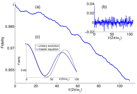
Figure 3: (a) Fidelity of coherent oscillations of the high-frequency mode in the linear trap ($\beta=85$). (b) $Re\langle\tilde{C}_{11}(\tau)\rangle$ of the same configuration. (c) Fidelity near a resonant configuration, using the master equation (blue), and a unitary evolution (dashed).

In order to analyze the dependence of the coherence on the trap parameter, we take the limit of a large circular trap with vanishing curvature, which is also the limit of a large linear trap with fixed ion density in the center. This is achieved using ‘periodic’ boundary conditions such that the longitudinal distance between any two ions is evaluated modulo half the chain length. The soliton configuration analyzed is of the same type as in Fig. 1(b). Figure 4(b) shows the fidelity as a function of $\gamma$ [which is independent of the number of ions, see Eq. 1]. The fidelity remains high provided that $\omega_{\rm low}$ is not too low [Fig. 4(a)], and that there is no strong resonance, $\omega_{1}\approx\omega_{j}+\omega_{\rm low}$, where the largest interaction coefficient is with $j=2$, a partly-localized phonon. The resonance on the left is seen to have a much weaker effect, owing to a smaller matrix-element. The loss of fidelity at the resonances is mainly due to energy relaxation from the high-frequency mode, while away from resonance the off-diagonal elements grow considerably, expressing the loss of phase coherence.

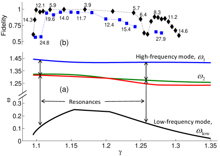
Figure 4: Mode frequencies and fidelity analysis. (a) The frequencies of the lowest and the three highest modes as a function of the trap parameter in the ’odd’ kink configuration (see text for details). (b) The lowest value of fidelity obtained for simulations of 50 oscillations of the high-frequency mode, at different parameter values. Black diamonds: at inter-ion separation of $1.5\mu{m}$. Blue squares: at twice that distance. The numbers indicate the population of thermal phonons in the low-frequency mode.

We continue with a discussion of various aspects of our treatment. The geometric coefficients $M_{ijkl}$ and successive terms omitted from the series expansion in eq. (2), are not necessarily decreasing compared with the third order $L_{ijk}$. However, powers of $\sqrt{\hbar}\sim 1/230$ dominate the convergence at low excitations, so already the contribution of quartic terms is negligible in general. The Hilbert space of the system is truncated at dimensions $8-10$, which we have checked to have negligible effect on the results because of the low phonon-numbers.

The dominant contribution to decoherence comes from multi-phonon processes involving the localized high and low modes. Powers of ${\omega_{\rm low}}^{-1/2}$ enter the coefficients of such interactions which grow stronger as $\omega_{\rm low}\to 0$. Since $\omega_{1}$ depends only weakly on the trap parameter (at a given kink type), while $\omega_{\rm low}$ and the gap are tunable, the highest fidelity is achieved at the center area of figure 4, where the gap is large and $\omega_{\rm low}$ is high and far from the strong resonances. These considerations hold when increasing $N$ at a given geometry, as the localized modes do not change their frequency or strength of local interactions. The number of all resonant processes grows proportionally to the phonon density ($\sim N$), but the strength of each one drops as $\sim 1/\sqrt{N}$ for every plane-wave phonon involved. This leaves only the weakly coupled third-order resonances, near $\omega_{j}\approx\omega_{1}-\omega_{\rm low}$, with a contribution scaling like $N/\sqrt{N}=\sqrt{N}$. In addition, there are the off-resonant couplings with phonons whose frequencies approach zero. Still, these two contributions will pose no problem up to at least a couple of hundreds of ions.

Production of kink configurations in the linear trap can be achieved by a fast temporal variation of the transverse potential. Numerical simulations indicate that this process together with simultaneous cooling indeed leads to creation of kinks [Fig. 1(b)], which remain stable at temperatures below $\sim 15T_{\rm Doppler}$.

Finally, our results should hold in other discrete nonlinear models. In particular, long coherence times have been obtained for the FK and discrete $\phi^{4}$ models [31].

To conclude, we have demonstrated that stable classical kink configurations exist in linear traps with $\gtrsim 20$ ions, as well as in circular traps. Our results suggest that coherence of solitonic internal modes is preserved for surprisingly long durations in Doppler cooled traps. The unique scale independent properties of the internal modes, specifically their gap separation from the phonon band, their localization to a few ions and their high frequency, suggest that such coherences can be measured and manipulated using existing ion trap techniques. This indicates that trapped-ion solitons may be useful for generating entanglement [11, 33, 32], and implementing quantum information processing in large systems.

B.R. acknowledges the support by Israeli Science Foundation grants 784/06, 920/09 and the Israeli German Foundation grant I-857. A.R. acknowledges the support of EPSRC project number EP/E045049/1. M.B.P. acknowledges support by the EU Integrated Project QAP, the Royal Society and an Alexander-von-Humboldt foundation.

References

- [1] R. Rajaraman, Solitons and Instantons, North Holland, Elsevier Science Publisher, Amsterdam (1982).
- [2] S. J. Carter, et al., Phys. Rev. Lett., 58, 1841 (1987). M. Rosenbluh and R. M. Shelby, Phys. Rev. Lett. 66, 153 (1991).
- [3] A. Wallraff et al., Nature 425, 155 (2003).
- [4] H. S. Eisenberg et al., Phys. Rev. Lett. 81, 3383 (1998).
- [5] J. W. Fleischer et al., Nature 422, 147 (2003).
- [6] A. Trombettoni and A. Smerzi, Phys. Rev. Lett. 86, 2353 (2001)
- [7] Ya. Frenkel and T. Kontorova, Phys. Z. Sowjetunion 13, 1 (1938).
- [8] O. M. Braun and Y. S. Kivshar, The Frenkel-Kontorova Model, Springer (2004).
- [9] O.M. Braun, Y.S. Kivshar and M. Peyrard, Phys. Rev. E 56, 6050 (1997).
- [10] A. J. Sievers and S. Takeno, Phys. Rev. Lett. 61, 970 (1988)
- [11] S. Marcovitch and B. Reznik, Phys. Rev. A 78, 052303 (2008).
- [12] For a recent review see, e.g., M. Šašura and V. Bužek, J. Mod Opt. 49, 1593 (2002).
- [13] D. Leibfried et al., Nature 438, 639 (2005).
- [14] H. Häffner et al., Nature 438, 643 (2005).
- [15] F. Mintert and C. Wunderlich, Phys. Rev. Lett.87 257904 (2001).
- [16] D. Porras and J.I. Cirac, Phys. Rev. Lett. 92, 207901 (2004).
- [17] A. Friedenauer et al., Nature Physics 4, 757 - 761 (2008).
- [18] D. Porras and J.I. Cirac, Phys. Rev. Lett. 93, 263602 (2004).
- [19] A. Retzker, J.I. Cirac and B. Reznik, Phys. Rev. Lett. 94, 050504 (2005). L. Lamata et al., Phys. Rev. Lett. 98, 253005 (2007).
- [20] P. M. Alsing, J. P. Dowling, and G. J. Milburn. Phys. Rev. Lett. 94, 220401 (2005). R. Schützhold et al., Phys. Rev. Lett. 99, 201301 (2007).
- [21] B. Horstmann et al., arXiv:0904.4801.
- [22] I. García-Mata et al., Eur. Phys. J. D 41, 325 (2007)
- [23] Oleg M. Braun, Yuri S. Kivshar, Phys. Rev. B 44, 7694 (1991). O. M. Braun et al., Phys. Rev. B 48, 3734 (1993).
- [24] D. H. E. Dubin and T. M. O’Neil, Rev. Mod. Phys. 71, 87 (1999).
- [25] S. Fishman et al.Phys. Rev. B77, 064111 (2008).
- [26] A. Retzker et al., Phys. Rev. Lett.101, 260504 (2008).
- [27] H. Carmichael, Statistical Methods in Quantum Optics, Springer-Verlag, Berlin (1999).
- [28] The small transverse departures of the ions are not expected to cause significant micromotion heating : B. E. King et al., Phys. Rev. Lett. 81, 1525 (1998).
- [29] For density operators and , .
- [30] S. Machnes, QLib, arXiv:quant-ph/0708.0478.
- [31] H. Landa, Master’s thesis, Tel Aviv University, arXiv:0910.0109.
- [32] R. K. Lee, Y. Lai and B. A. Malomed, Phys. Rev. A 71, 013816 (2005).
- [33] M. Lewenstein and B. A. Malomed, arXiv:0901.2836 [New J. Phys. (to be published)].