Beauty baryon production in $pp$ collisions at LHC and $b$ quark distribution in proton

Abstract

The production of charmed and beauty hadrons in proton-proton and proton-antiproton collisions at high energies are analyzed within the modified quark-gluon string model (QGSM) including the internal motion of quarks in colliding hadrons. We present some predictions for the future experiments on the beauty baryon production in $pp$ collisions at LHC energies. This analysis allows us to find interesting information on the Regge trajectories of the heavy ($b{\bar{b}}$) mesons and the sea beauty quark distributions in the proton.

1 Introduction

Various approaches of perturbative QCD including the next-to-leading order calculations (NLO QCD) have been applied to construct distributions of quarks in a proton. The theoretical analysis of the lepton deep inelastic scattering (DIS) off protons and nuclei provides rather realistic information on the distribution of light quarks like $u,d,s$ in a proton. However, to find a reliable distribution of heavy quarks like $c({\bar{c}})$ and especially $b({\bar{b}})$ in a proton describing the experimental data on the DIS is a non-trivial task. It is mainly due to small values of $D$ and $B$ meson yields in the DIS at existing energies. Even at the Tevatron energies the $B$- meson yield is not so large. At LHC energies the multiplicity of these mesons produced in $pp$ collisions will be significantly larger. Therefore one can try to extract a new information on the distribution of these heavy quarks in a proton. In this paper we suggest to study the distribution of heavy quarks like $c({\bar{c}})$ and $b({\bar{b}})$ in a proton from the analysis of the future LHC experimental data.

The multiple hadron production in hadron-nucleon collisions at high energies and large transfers is usually analyzed within the hard parton scattering model (HPSM) suggested in [1, 2]. This model was applied to the charmed meson production both in proton-proton and meson-proton interactions at high energies, see for example [3]. The HPSM is significantly improved by applying the QCD parton approach [4, 5], see details in [6] and references therein. Unfortunately the QCD including the next-to-leading order (NLO) has some uncertainties related to the renormalization parameters especially at small transverse momenta $p_{t}$ [6].

In [6, 7] we studied the charmed and beauty meson production in $pp$ and $p{\bar{p}}$ collisions at high energies within the QGSM [8] or the dual parton model (DPM) [9] based on the $1/N$ expansion in QCD [10, 11]. It was shown that this approach can be applied rather successfully at not very large values of $p_{t}$. In this paper we investigate the open charm and beauty baryon production in $pp$ collisions at LHC energies and very small $p_{t}$ within the QGSM to find new information on the Regge trajectories of the heavy ($c{\bar{c}}$) and ($b{\bar{b}}$) mesons and the sea beauty quark distributions in the proton.

2 General formalism for hadron production in $pp$ collision within QGSM

Let us present briefly the scheme of the analysis of the hadron production in the $pp$ collisions within the QGSM including the transverse motion of quarks and diquarks in colliding protons [12]. As is known, the cylinder type graphs for the $pp$ collision presented in Fig.1 make the main contribution to this process [8]. The left diagram of Fig.1, the so-called one-cylinder graph, corresponds to the case where two colorless strings are formed between the quark/diquark ($q/qq$) and the diquark/quark ($qq/q$) in colliding protons; then, after their breakup, $q{\bar{q}}$ pairs are created and fragmentated to a hadron, for example, $D$ meson. The right diagram of Fig.1, the so-called multicylinder graph, corresponds to creation of the same two colorless strings and many strings between sea quarks/antiquarks $q/{\bar{q}}$ and sea antiquarks/quarks ${\bar{q}}/q$ in the colliding protons.

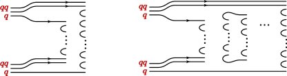
Figure 1: The one-cylinder graph (left diagram) and the multicylinder graph (right diagram) for the inclusive $pp\rightarrow hX$ process.

The general form for the invariant inclusive hadron spectrum within the QGSM is [13, 12]

$$E\frac{d\sigma}{d^{3}{\bf p}}\equiv\frac{2E^{*}}{\pi\sqrt{s}}\frac{d\sigma}{dxdp_{t}^{2}}=\sum_{n=1}^{\infty}\sigma_{n}(s)\phi_{n}(x,p_{t})~{},$$ (1)

where $E,{\bf p}$ are the energy and the three-momentum of the produced hadron $h$ in the laboratory system (l.s.) of colliding protons; $E^{*},s$ are the energy of $h$ and the square of the initial energy in the c.m.s of $pp$; $x,p_{t}$ are the Feynman variable and the transverse momentum of $h$; $\sigma_{n}$ is the cross section for production of the $n$-Pomeron chain (or $2n$ quark-antiquark strings) decaying into hadrons, calculated within the “eikonal approximation” [14]. Actually, the function $\phi_{n}(x,p_{t})$ is the convolution of the quark (diquark) distributions in the proton and their fragmentation functions (FF) , see details in [8, 9, 6, 12]. To calculate the interaction function $\phi_{n}(x,p_{t})$ we have to know all the quark (diquak) distribution functions in the nth Pomeron chain and the FF. They are constructed within the QGSM using the knowledge of the secondary Regge trajectories, see details in [8, 13].

3 Heavy baryon production within QGSM

3.1 Sea charm and beauty quark distribution in proton

Now let us analyze the charmed and beauty baryon production in the $pp$ collision at LHC energies and very small $p_{t}$ within the soft QCD, e.g., the QGSM. This study can be interesting for it may allow predictions for future LHC experiments like TOTEM and ATLAS and an opportunity to find new information on the distribution of sea charmed ($c$) and beauty ($b$) quarks at very low $Q^{2}$. According to the QGSM, the distribution of $c({\bar{c}})$ quarks in the $n$th Pomeron chain (Fig.1(right)) is, see for example [12] and references therein,

$$f_{c({\bar{c}})}^{(n)}(x)=C_{c({\bar{c}})}^{(n)}\delta_{c({\bar{c}})}x^{a_{cn}}(1-x)^{g_{cn}}\quad$$ (2)

where $a_{cn}=-\alpha_{\psi}(0)$, $g_{cn}=\alpha_{\rho}(0)-2\alpha_{B}(0)+(\alpha_{\rho}(0)-\alpha_{\psi}(0))+n-1$; $\delta_{c({\bar{c}})}$ is the weight of charmed pairs in the quark sea, $C_{c({\bar{c}})}^{(n)}$ is the normalization coefficient [13], $\alpha_{\psi}(0)$ is the intercept of the $\psi$- Regge trajectory. Its value can be $-2.18$ assuming that this trajectory $\alpha_{\psi}(t)$ is linear and the intercept and the slope $\alpha_{\psi}^{\prime}(0)$ can be determined by drawing the trajectory through the $J/\Psi$-meson mass $m_{J/\Psi}\simeq 3.1$ GeV and the $\chi$-meson mass $m_{\chi}=3.554$ GeV [15]. Assuming that the $\psi$- Regge trajectory is nonlinear one can get $\alpha_{\psi}(0)\simeq 0$, which follows from perturbative QCD, as it was shown in [16]. The distribution of $b({\bar{b}})$ quarks in the $n$th Pomeron chain (Fig.1(right)) has the similar form

$$f_{b({\bar{b}})}^{(n)}(x)=C_{b({\bar{b}})}^{(n)}\delta_{b({\bar{b}})}x^{a_{bn}}(1-x)^{g_{bn}}\quad$$ (3)

where $a_{bn}=-\alpha_{\Upsilon}(0)$, $g_{bn}=\alpha_{\rho}(0)-2\alpha_{B}(0)+(\alpha_{\rho}(0)-\alpha_{\Upsilon}(0))+n-1$; $\alpha_{\rho}(0)=1/2$ is the well known intercept of the $\rho$-trajectory; $\alpha_{B}(0)\simeq-0.5$ is the intercept of the baryon trajectory, $\alpha_{\Upsilon}(0))$ is the intercept of the $\Upsilon$- Regge trajectory, its value also has an uncertainty. Assuming its linearity one can get $\alpha_{\Upsilon}(0))=-8,-16$, while for nonlinear ($b{\bar{b}}$) Regge trajectory $\alpha_{\Upsilon}(0)\simeq 0$, see details in [17]. Inserting these values to the form for $f_{c({\bar{c}})}^{(n)}(x)$ and $f_{b({\bar{b}})}^{(n)}(x)$ we get the large sensitivity for the $c$ and $b$ sea quark distributions in the $n$th Pomeron chain. Note that the FFs also depend on the parameters of these Regge trajectories. Therefore, the knowledge of the intercepts and slopes of the heavy-meson Regge trajectories is very important for the theoretical analysis of open charm and beauty production in hadron processes.

Note that all the quark distributions obtained within the QGSM are different from the parton distributions obtained within the perturbative QCD which are usually compared with the experimental data on the deep inelastic lepton scattering (DIS) off protons. To match these two kinds of quark distributions one can apply the procedure suggested in [18]. The quantities $g_{cn}$ or $g_{bn}$ entering into Eq.(2) and Eq.(3) are replaced by the following new quantities depending on $Q^{2}$

$${\tilde{g}}_{cn}=g_{cn}(1+\frac{Q^{2}}{Q^{2}+c})~{};~{}{\tilde{g}}_{bn}=g_{bn}\left(1+\frac{Q^{2}}{Q^{2}+d}\right)$$ (4)

The parameters $c$ and $d$ are chosen such that the structure function constructed from the valence and sea quark (antiquark) distributions in the proton should be the same as the one at the initial conditions at $Q^{2}=Q_{0}^{2}$ for the perturbative QCD evolution.A similar procedure can be used to get the $Q^{2}$ dependence for the powers $a_{cn}$ and $a_{bn}$ entering into Eqs.(2,3) [18]. Then using the DGLAP evolution equation [19] we obtain the structure functions at large $Q^{2}$.

3.2 Charmed and beauty baryon production in $pp$ collision

The information on the charmonium ($c{\bar{c}}$) and botomonium ($b{\bar{b}}$) Regge trajectories can be found from the experimental data on the charmed and beauty baryon production in $pp$ collisions at high energies. For example, Fig.2 illustrates the sensitivity of the inclusive spectrum $d\sigma/dx$ of the produced charmed baryons $\Lambda_{c}$ to different values for $\alpha_{\psi}(0)$. The solid line corresponds to $\alpha_{\psi}(0)=0$, whereas the dashed curve corresponds to $\alpha_{\psi}(0)=-2.18$. Unfortunately the experimental data presented in Fig.2 have big uncertainties; therefore, one cant extract the information on the $\alpha_{\psi}(0)$ values from the existing experimental data.

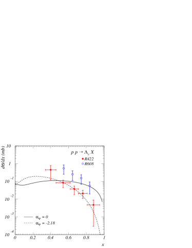
Figure 2: The differential cross section $d\sigma/dx$ for the inclusive process $pp\rightarrow\Lambda_{c}X$ at $\sqrt{s}=62~{}\mathrm{GeV}$.

A high sensitivity of the inclusive spectrum $d\sigma/dx$ of the produced beauty baryons $\Lambda_{b}$ to different values for $\alpha_{\Upsilon}(0)$ is presented in Fig.3 (left).

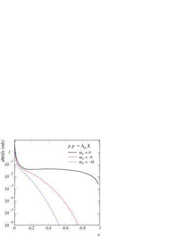
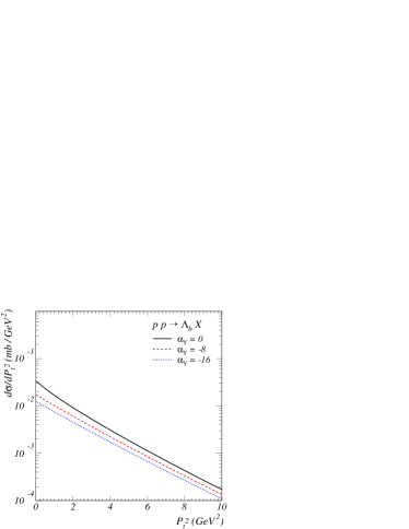
Figure 3: The differential cross section $d\sigma/dx$ (left) and $d\sigma/dP_{t}^{2}$ (right) for the inclusive process $pp\rightarrow\Lambda_{b}X$ at $\sqrt{s}=4~{}\mathrm{TeV}$.

The $p_{t}$-inclusive spectrum of $\Lambda_{b}$ has much lower sensitivity to this quantity, according to the results presented in Fig.3 (right). Actually, our results presented in Fig.3 could be considered as some predictions for future experiments at LHC, see Fig.4.

Now let us analyze the production of the beauty hyperon, namely $\Lambda^{0}_{b}$, at small scattering angles $\theta_{\Lambda^{0}_{b}}$ in the $pp$ collision at LHC energies. This study would be reliable for the future forward experiments at LHC. The produced $\Lambda^{0}_{b}$ baryon can decay as $\Lambda^{0}_{b}\rightarrow J/\Psi\Lambda^{0}$, and $J/\Psi$ decays into $\mu^{+}\mu^{-}$, its branching ratio ($Br=\Gamma_{j}/\Gamma$) is $5.93\pm 0.06$ percent, or into $e^{+}e^{-}$ ($Br=5.93\pm 0.06\%$), whereas $\Lambda^{0}$ can decay into $p\pi^{-}$ ($Br=\Gamma_{j}/\Gamma=63.9\pm 05\%$), or into $n\pi^{0}$ ($Br=35.8\pm 0.5\%$), see Fig.4.

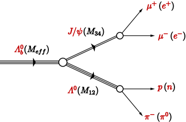
Figure 4: The decay $\Lambda_{b}\rightarrow J\Psi~{}\Lambda^{0}\rightarrow\mu^{+}\mu^{-}(e^{+}e^{-})~{}p\pi^{-}(n\pi^{0})$.

$$\frac{d\sigma}{d^{3}p_{1}dM_{34}}=\int\frac{d\sigma}{dM_{12}dM_{34}}$$ (5)

$$\delta^{(3)}({\bf p}_{1}+{\bf p}_{2}-{\bf p}_{12})dM_{12}~{},$$

where

$$\frac{d\sigma}{dM_{12}dM_{34}}=\int d^{2}p_{t\Lambda_{b}}\frac{d\sigma_{pp\rightarrow\Lambda_{b}X}}{dxd^{2}p_{t\Lambda_{b}}}$$

$$Br_{\Lambda_{b}\rightarrow J/\Psi}Br_{J/\Psi\rightarrow\mu^{+}\mu_{-}}Br_{\Lambda^{0}\rightarrow p\pi}\frac{\pi^{3}}{2M^{2}_{eff}M_{12}M_{34}}$$

$$\lambda^{1/2}(M^{2}_{eff},M^{2}_{12},M^{2}_{34})\lambda^{1/2}(M^{2}_{12},M^{2}_{1},M^{2}_{2})\lambda^{1/2}(M^{2}_{34},M^{2}_{3},M^{2}_{4})~{},$$

$Br_{\Lambda_{b}\rightarrow J/\Psi}=(4.7\pm 2.8)\cdot 10^{-4};~{}Br_{J/\Psi\rightarrow\mu^{+}\mu_{-}}=(5.93\pm 0.06)\%;~{}Br_{\Lambda^{0}\rightarrow p\pi}=(63.9\pm 0.5)\%$.
Here $\lambda(x^{2},y^{2},z^{2})=((x^{2}-(y+z)^{2})((x^{2}-(y-z)^{2})$
One can get the following relation

$$d^{3}p_{1}~{}=~{}\frac{1}{2}p\xi_{p}d\phi_{1}d\xi_{p}dt_{p}~{},$$ (6)

where $\xi_{p}=\Delta p/p$ is the energy loss, $t_{p}=(p_{in}-p_{1})^{2}$ is the four-momentum transfer, $\phi_{1}$ is the azimuthal angle of the final proton with the three-momentum ${\bf p}_{1}$.
Experimentally one can measure the differential cross section

$$\frac{d\sigma}{d\xi_{p}dt_{p}dM_{J/\Psi}}~{}=~{}\frac{1}{2}p\xi_{p}\int\frac{d\sigma}{d^{3}p_{1}dM_{34}}d\phi_{1}$$ (7)

This distribution could be reliable for the TOTEM experiment, where $J/\Psi$ decays into $\mu^{+}\mu^{-}$ and $\Lambda^{0}_{b}$ decays into $\pi^{-}p$ or for the ATLAS forward experiment, where $\Lambda^{0}_{b}$ decays as $\Lambda^{0}_{b}\rightarrow J/\Psi~{}\Lambda^{0}\rightarrow e^{+}e^{-}~{}\pi^{0}n$ (Fig.4).

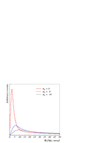
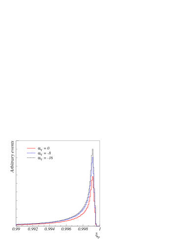
Figure 5: The distributions over $\theta_{J/\Psi}$ (left) and $\xi_{p}$ (right) for the inclusive process $pp\rightarrow\Lambda_{b}X\rightarrow\mu^{+}\mu^{-}p\pi^{-}X$ at $\sqrt{s}=4.$ TeV

In Fig.5 the distributions over $\theta_{J/\Psi}$ (left) and $\xi_{p}$ (right) are presented at different values of the intercept $\alpha_{\Upsilon}(0)=0$ (solid line), $\alpha_{\Upsilon}(0)=-8$ (dashed line) and $\alpha_{\Upsilon}(0)=-16$ (dotted line), where $\theta_{J/\Psi}$ is the scattering angle for the final $J/\Psi$. Fig.5 shows a sensitivity of these distributions to the intercept of the $\alpha_{\Upsilon}$ Regge trajectory. Actually, the result presented in Fig.5 is a prediction for future LHC experiments on the heavy flavour baryon production at the LHC energies.

4 Conclusion

It was shown [6, 7] that the modified QGSM including the intrinsic longitudinal and transverse motion of quarks (antiquarks) and diquarks in colliding protons allowed us to describe rather satisfactorily the existing experimental data on inclusive spectra of heavy hadrons produced in $pp$ and $p{\bar{p}}$ collisions It allows us to make some predictions for future LHC forward experiments on the beauty baryon production in $pp$ collisions which can give us new information on the beauty quark distribution in the proton and very interesting information on the Regge trajectories of ($b{\bar{b}}$) mesons.

5 Acknowledgments

We thank M. Deile, K. Eggert, D. Elia, P. Garfström, A. B. Kaidalov, A. D. Martin, M. Poghosyan and N. I. Zimin for very useful discussions. This work was supported in part by the RFBR grant N 08-02-01003.

References

- [1] A.V. Efremov, Yad. Fiz. 19 179 (1974).
- [2] R.D. Field and R.P. Feyman, Phys. Rev. D15 2590 (1977); R.D. Field, R.P. Feyman and G.C. Fox, Nucl. Phys. B128 1 (1977).
- [3] V.A. Bednyakov V.A., Mod.Phys.Lett. A10 61 (1995).
- [4] P. Nasson, S. Dawson and R.K. Ellis, Nucl. Phys. B303 607 (1988); ibid. B327 49 (1989); ibid. B335 260E (1989).
- [5] B.A. Kniehl and G. Kramer, Phys.Rev. D60 014006 (1999).
- [6] G.I. Lykasov, Z.M. Karpova, M.N. Sergeenko and V.A. Bednyakov, Europhys.Lett. 86 61001 (2009); arXiv:hep-ph/0812.3220 (2009).
- [7] G.I. Lykasov, V.V. Lyubushkin and V.A. Bednyakov, arXiv:hep-ph/0909.5061 (2009).
- [8] A.B. Kaidalov, Phys. Lett. B116 459 (1982); A.B. Kaidalov and K. A. Ter-Martirosyan, Phys. Lett. B117 247 (1982).
- [9] A. Capella, U. Sukhatme, C. I. Tan, J. Tran Than Van, Phys. Rep. 236 225 (1994).
- [10] G. t’Hooft, Nucl.Phys. B72 461 (1974).
- [11] G. Veneziano, Phys. Lett. B52 220 (1974).
- [12] G.I. Lykasov, G.H. Arakelian and M.N. Sergeenko, Phys. Part. Nucl. 30 343 (1999); G.I. Lykasov, M.N. Sergeenko, Z. Phys. C70 455 (1996).
- [13] A.B. Kaidalov and O.I. Piskunova, Z. Phys. C30 145 (1986).
- [14] K.A. Ter-Martirosyan, Phys. Lett. B44 (1973) 377.
- [15] K.G. Boreskov, A.B. Kaidalov, Sov.J.Nucl.Phys. 37 100 (1983).
- [16] A.B. Kaidalov, O.I. Piskunova, Sov.J.Nucl.Phys. 43 994 (1986).
- [17] O.I Piskunova, Yad. Fiz. 56 176 (1993) (Phys.Atom.Nucl. 56 1094 (1993); ibid 64 392 (2001).
- [18] A. Capella, A.B. Kaidalov, C. Merino and J. Tran Than Van, Phys.Lett. B337 358(1994); ibid B343 403 (1995).
- [19] V.N. Gribov and L.N. Lipatov, Sov.J.Nucl.Phys. 15 438 (1972) ; G. Altarelli and G. Parisi, Nucl.Phys. B126 298 (1977); Yu.L. Dokshitzer, Sov.Phys. JETP 46 641 (1977).