Effect of Ad-Hoc Vehicular Network on Traffic Flow: Simulations in the Context of Three-Phase Traffic Theory

Abstract

Effects of vehicle-to-vehicle (or/and vehicle-to-infrastructure communication, called also V2X communication) on traffic flow, which are relevant for ITS, are numerically studied. To make the study adequate with real measured traffic data, a testbed for wireless vehicle communication based on a microscopic model in the framework of three-phase traffic theory is developed and discussed. In this testbed, vehicle motion in traffic flow and analyses of a vehicle communication channel access based on IEEE 802.11 mechanisms, radio propagation modeling, message reception characteristics as well as all other effects associated with ad-hoc networks are integrated into a three-phase traffic flow model. Thus simulations of both vehicle ad-hoc network and traffic flow are integrated onto a single testbed and perform simultaneously. This allows us to make simulations of ad-hoc network performance as well as diverse scenarios of the effect of wireless vehicle communications on traffic flow during simulation times, which can be comparable with real characteristic times in traffic flow. In addition, the testbed allows us to simulate cooperative vehicle motion together with various traffic phenomena, like traffic breakdown at bottlenecks, moving jam emergence, and a possible effect of danger warning massages about the breakdown vehicle on traffic flow.

1 Introduction

Wireless vehicle communication, which is the basic technology for ad-hoc vehicle networks, is one of the most important scientific fields of future ITS. This is because there are many possible applications of ad-hoc vehicle networks, including various systems for danger warning, traffic adaptive assistance systems, traffic information and prediction in vehicles, improving of traffic flow characteristics through adaptive traffic control, etc. [1, 2, 3, 4, 5, 6, 7]. However, the evaluation of ad-hoc vehicle networks requires many communicating vehicles moving in real traffic flow, i.e., field studies of ad-hoc vehicle networks are very complex and expensive. For this reason, to prove the performance of ad-hoc vehicle networks based on wireless vehicle communication, reliable simulations of ad-hoc vehicle networks are of great importance and indispensable.

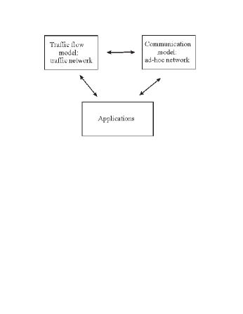
Figure 1: Usual scheme of testbeds for simulations of ad-hoc vehicle networks (e.g., [9, 10, 11, 12, 13, 14, 15, 16, 17]).

An usual schema for the development of a testbed for simulations of ad-hoc vehicle networks includes a traffic flow model, a model for vehicle communications that is often based on the use of ns-2 simulator [8], and application models (applications in Fig. 1) (e.g., [9, 10, 11, 12, 13, 14, 15, 16, 17]). Application models determine, for example, necessary changes in vehicle behavior in traffic flow after receiving of the associated message or/and whether this message should be resent to other vehicles or not. There are two different networks in such testbeds: (i) a traffic network simulated with the use of the traffic flow model and (ii) a communication (ad-hoc) network simulated with the use of the communication model in which positions and other characteristics of each communicated vehicle are taken from simulations of the traffic network made at the latest point in time. Simulations of many communicating vehicles in the communication network with known communication models are very time intensive. For this reason, often the model of communication network (communication model in Fig. 1) performs simulations based on traffic flow data previously simulated through the use of the traffic flow model (off-line simulations of traffic networks). In some of these testbeds, to study applications in which vehicle behavior should be changed in accordance with received messages, the communication model performs simulations after each time step of traffic flow simulations. In any case, the use of this simulation schema (Fig. 1) requires a very long run time of the simulations, which can be some order of magnitude longer than real time of vehicle moving in traffic flow.

In this article, we perform a numerical study of possible effects of vehicle-to-vehicle or/and vehicle-to-infrastructure communication (called also V2X communication) on traffic flow. To make the study adaquate with real measured traffic data, a testbed for wireless vehicle communication based on a microscopic model in the framework of three-phase traffic theory is developed and discussed. In this testbed, simulations of a traffic network and an ad-hoc vehicle network as well as applications are integrated into an united network, i.e., there is only one network in this testbed. The network describes both vehicle motion in traffic flow and communications as well as the effect of applications on traffic flow and vehicle behavior. As a result, simulations of ad-hoc performance and various applications can be made many times quicker than with the scheme shown in Fig. 1. To reach this goal, each vehicle in this network exhibit different attributes needed for both vehicle motion and communications, and application scenarios. In addition, we should note that recently based on a study of measured data on many highways in different countries a three-phase traffic theory has been developed. In contrast with earlier traffic flow theories and models, three-phase traffic theory can explain and predict all known empirical features of traffic breakdown and resulting congested patterns [22, 23]. For this reason, we use a traffic flow model in the framework of three-phase traffic theory. A model for vehicle ad-hoc network is presented in Sect. III. Simulations of three scenarios of C2C application devoted to ad-hoc network influence on traffic flow are presented in Sects. IV–VI, respectively. However, in section $``$Backgroughs” we briefly consider channel access mechanism used for simulations of vehicle communication (Sect. 2.1) and some features of three-phase traffic theory used for traffic simulations (Sect. 2.2).

2 Backgrounds

2.1 Channel Access Mechanism used for Simulations of Vehicle Communication

If there are messages to be sent and the medium is free, the vehicle sends the message that has the highest priority and/or is the first one in the message queue in this vehicle. To prevent collisions between messages sent by different communicating vehicles, a message access method is usually applied.

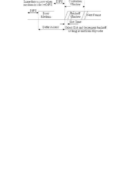
Figure 2: IEEE 802.11 basic access mechanism [19, 20, 21]

As an example, we use here IEEE 802.11e basic access method [19, 20, 21]. No access is possible when medium is busy. After the medium has been free, in accordance with the IEEE 802.11e access method, there is a backoff procedure applied for each of the communicating vehicles independently of each other. At the end of the backoff procedure, a decision whether the medium is free or busy is made.

In accordance with IEEE 801.11e mechanism, we can summarize possible cases as follows:

(i) None of the signal powers in the matrix is greater than a signal receiving threshold (RXTh); then no message is accepted. Under this condition, there can be two possible cases:

(a) The sum of all signal powers in the matrix is smaller than the carrier sense threshold CSTh. Then the medium is free; therefore, the abovementioned backoff procedure is applied for the message sending (Fig. 2).

(b) The sum of all signal powers in the matrix is equal to or greater than the threshold CSTh. Then the medium is busy for the vehicle.

(ii) The greatest signal power of the signal powers in the matrix is greater than the threshold RXTh. Under this condition, it is tested for the matrix of signal powers whether the ratio between the power of this greatest signal power and the sum of the powers of all other signals stored in the matrix is greater than the required signal-to-noise ratio (SNR) at the selected data rate (DR) for the whole duration of the message: 1) If yes, then the signal could be considered to be received. 2) Otherwise, there is no message acceptance at this time instance.

2.2 Three-Phase Traffic Theory – The Basis for Update Rules of Vehicle Motion

There are three phases in three-phase traffic theory [22]:

• Free flow (F).

• Synchronized flow (S).

• Wide moving jam (J).

The synchronized flow and wide moving jam traffic phases are associated with congested traffic.

The empirical study of real measured traffic data mentioned above shows that there are common pattern features that are qualitatively the same independent of highway infrastructure, weather, percentage of long vehicles, vehicle technology, etc. The empirical traffic phase definitions [S] and [J] for the synchronized flow and wide moving jam phases in congested traffic made in three-phase traffic theory are these common empirical pattern features.

The definition of the wide moving jam phase [J]: A wide moving jam is a moving jam that maintains the mean velocity of the downstream jam front, even when the jam propagates through other traffic phases or bottlenecks.

The definition of the synchronized flow phase [S]: In contrast with the wide moving jam phase, the downstream front of the synchronized flow phase does not exhibit the wide moving jam characteristic feature; in particular, the downstream front of the synchronized flow phase is often fixed at a bottleneck.

Recall that a moving jam is a propagating upstream localized structure of great vehicle density and very low speed spatially limited by two jam fronts. Within the downstream jam front vehicles accelerate escaping from the jam; within the upstream jam front, vehicles slow down approaching the jam.

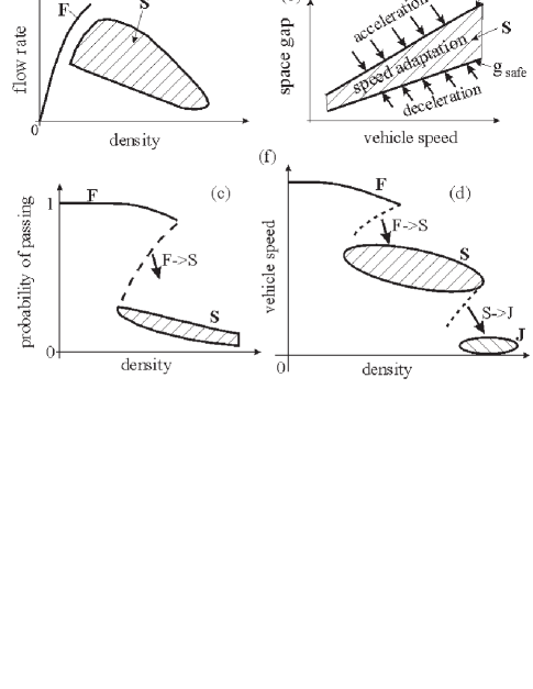
Figure 3: Hypotheses of three-phase traffic theory about traffic breakdown and wide moving jam emergence [22].

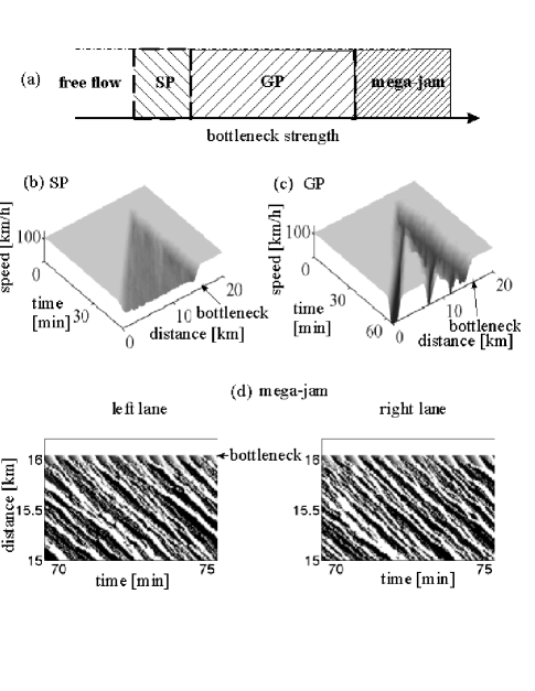
Figure 4: Hypotheses of three-phase traffic theory about congested traffic patterns resulting from traffic breakdown: (a) Simplified diagram of congested patterns. (b–d) SP (b), GP (c), and mega-jam (d). In (d), within black regions vehicles are in standstill, whereas within white regions vehicles move at very low speeds within the mega-jam [22, 23].

The phase definitions [S] and [J] in real measured traffic data are the empirical basis of hypotheses of three-phase traffic theory inmlemented into mathematical three-phase traffic flow models. Some of these hypotheses are as follows:

(1) Rather than a fundamental diagram, in three-phase traffic theory steady states of synchronized flow cover a two-dimensional (2D) region in the flow–density plane (dashed region in Fig. 3 (a)): While adapting speed to the speed of the preceding vehicle, a driver accepts different space gaps within a limited gap range $g_{\rm safe}\leq g\leq G$, where $G$ and $g_{\rm safe}$ are some synchronization and safe space gaps, respectively (Fig. 3 (b))).

(2) Traffic breakdown at a highway bottleneck is a local phase transition from free flow to synchronized flow (F$\rightarrow$S transition). Traffic breakdown is explained by a Z-shaped density function of probability of vehicle passing (Fig. 3 (c)): There is a drop in this probability when free flow transforms into synchronized flow.

(3) In free flow, wide moving jams emerge due to a sequence of F$\rightarrow$S$\rightarrow$J transitions that can be illustrated by a double Z-characteristic (Fig. 3 (d)). The first Z-shaped relationship, which includes free flow $F$ and synchronized flow $S$, is associated with an F$\rightarrow$S transition, i.e., traffic breakdown (labeled by arrows F$\rightarrow$S in Figs. 3 (c, d)). The second Z-shaped relationship, which includes synchronized flow $S$ and low speed states within wide moving jams $J$, is associated with an S$\rightarrow$J transition (labeled by arrow S$\rightarrow$J in Fig. 3 (d)).

(4) If the bottleneck strength, which characterizes the influence of a bottleneck on traffic breakdown and resulting traffic congestion, increases gradually, firstly a synchronized flow pattern (SP) emerges upstream of the bottleneck (Fig. 4 (a, b)). Congested traffic within an SP consists of synchronized flow only. At a greater bottleneck strength, the SP transforms into a general congested pattern (GP) (Fig. 4 (a, c)). Congested traffic within an GP consists of synchronized flow and wide moving jams that emerge in synchronized flow. If the bottleneck strength increases further, the GP transforms into a mega-wide moving jam (mega-jam) (Fig. 4 (a, d)).

3 United Ad-Hoc Network Model

In the united network model of traffic flow, C2C-comunications, and ad-hoc networks, there are dynamic vehicle attributes, which exhibit each of the communicating vehicles (Fig. 5). All other vehicles in the network, which cannot communicate, exhibit only one dynamic attribute: update rules for vehicle motion. If in addition with communicating vehicles the network includes roadside communication units (RSU), each RSU exhibits the communicating vehicle attributes with the exception of the update rules for vehicle motion.

3.1 Update Rules for Vehicle Motion

The vehicle attribute $``$update rules for vehicle motion” are given by a stochastic microscopic three-phase traffic flow model of Kerner and Klenov [24, 25], which as shown in [22, 23] can explain all fundamental measured spatiotemporal features of real traffic flow. Because the detailed model description can be found in [22], basic rules of vehicle motion in the model are in Appendix A.

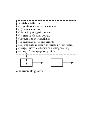
Figure 5: Scheme of simulations of ad-hoc networks and traffic flow within a united network model.

3.2 Message Access

During a motion of a communicating vehicle in a traffic network, the vehicle (and RSU) attribute $``$message access” calculates vehicle access possibility for message sending for each vehicle independent of each other in an unsynchronous manner, i.e., in contrast with update rules of vehicle motion no fixed time discretization is used in the model of vehicle communication. In the version of the testbed, we use IEEE 802.11e basic access method of Sect. 2.1.

3.3 Radio Propagation Model

Based on the vehicle (and RSU) attribute $``$radio propagation model”, signal powers of the message that has been sent by the vehicle are calculated for current locations of all other communicating vehicles and RSUs.

There are many different radio propagation models. However, at a time instant the real signal power of the message sent by a vehicle at a location of another communicating vehicle can be an extremely complex function of urban infrastructure (e.g., whether there are buildings causing strong signal reflection effects), the current vehicle distribution on the road (e.g., how many vehicles are between the vehicle and the location as well as whether there are long-vehicles between the vehicle and location at which the signal power should be found), etc.

One of the approaches to solve this complex problem is as follows. In our model, each communicating vehicle can apply either one of many radio propagation models stored in the vehicle or one of the different parameters of a radio propagation model. At a given time instant, the choice of the radio propagation model or the model parameter occurs automatically for each vehicle individually and independently of radio propagation models used by other vehicles. This radio propagation model choice is based on the current vehicles’ distribution on the road (and if known, urban infrastructure). Because a set of radio propagation models and their variable parameters stored in vehicles should cover diverse scenarios of different urban infrastructures and vehicle distributions, the radio propagation models should be associated with field study measurements made in accordance with these possible different scenarios. Unfortunately, at this time there is no such detailed experimental basis for the development of the model set available.

For this reason, as long as the abovementioned experimental basis is not available, in simulations we use one of the simplest radio propagation models – a well-known two-ray-ground radio propagation model

$$P(R)=P_{0}(R_{0}/R)^{m},$$ (1)

where $R_{0}$ is a communication range, $m$ is a model parameter that is $m\geq 2$, $R$ is the distance between two communicating vehicles, $P$ is the signal power, $P_{0}$ is constant.

In (1), the communication range $R_{0}$ and value $m$ are in general time-dependent model parameters. This is because $R_{0}$ and $m$ depend on the current vehicles’ distribution on the road as well as on urban characteristics (e.g., buildings and other obstacles in the neighberhood of the road) causing the reflection, diffraction, and other effects that influence on the signal power. Because the vehicle distribution on the road and some urban characteristics can randomly change over time during vehicle motion, the values $R_{0}$ and $m$ in (1) can be stochastic time variables. Time-dependencies of $R_{0}$ and $m$ in (1) for different vehicles can be very different. Nevertheless, due to vehicle motion we can expect that mean characteristics of the stochastic variables of $R_{0}$ and $m$ in (1) can be the same for different communicating vehicles.

3.4 Matrix of Signal Powers

In the model (Fig. 5), to make the decision whether the medium is free or busy or else the vehicle has received a message or not, based on the vehicle attribute $``$radio propagation model” [18], signal powers of messages sent by all other communicating vehicles are calculated. If a signal power is greater than a given threshold signal power denoted by $P_{\rm th}$ (model parameter), then this signal power of the associated message is stored into a $``$matrix of signal powers” of the vehicle:

• at each time instant, the matrix of signal powers of the vehicle contains signal powers of messages sent by other vehicles in ad-hoc network that are greater than the threshold signal power $P_{\rm th}$ at the location of the vehicle.

This threshold $P_{\rm th}$ is chosen to be much smaller than a carrier sense threshold (CSTh). The smaller $P_{\rm th}$ is chosen, the greater the accuracy of simulations of ad-hoc network performance, however, the longer the simulations run time. Signal reception characteristics (whether the medium is free or busy as well as whether the vehicle has received a message or not) are associated with an analysis of the matrix of signal powers, which is automatically made at each time instant for each communicating vehicle individually. The decision about signal collisions is further used for a study of ad-hoc network performance.

Table 1: Hypothetical example for matrix of signal powers

ID of sending
vehicle	25	382	37	36	31
Distance (in [m])
between
the receiving	234	345	300	70	562
vehicle 33 and
sending vehicle
Received signal
power (in [dBm])
of the message	$-$ 91	$-$ 95	$-$ 93	$-$ 81	$-$ 99
sent at the location
of the vehicle 33

We consider an application of the matrix of signal powers for a hypothetical example of a communicating vehicle with a vehicle-ID (identification number) 33 (Table 1). In this case, in the matrix of the vehicle 33 there are several signal powers of those messages sent at the time $t$ by other vehicles in an ad-hoc network whose signal powers are greater than the threshold CSTh $=-$ 96 dBm at the location of the vehicle 33. However, only the signal power of a message sent by vehicle ID 36 that is equal to $-$ 81 dBm is greater than a signal receiving threshold RXTh $=-$ 90 dBm. The ratio between the power of this greatest signal power of a message sent by vehicle ID 36 and the sum of the powers of all other signals stored in the matrix is greater than the required signal-to-noise ratio (SNR) for the whole duration of the message. Thus in the matrix of signal powers the signal sent by vehicle 36 that is 70 m outside of the location of vehicle 33 could be considered to be received by vehicle 33.

3.5 Reception Characteristics

Signal reception characteristics are associated with an analysis of the matrix of signal powers of Sect. 3.4, which is automatically made at each time instant for each communicating vehicle individually. In particular, this matrix is used for the decision whether the medium is free or busy at each time instant as well as for the decision whether the vehicle has received a message or not.

We see that at each time instant the matrix of signal powers is used both for the decision whether the vehicle has received a message and whether there are collisions between two or more different signals at the current vehicle location. Message collisions are realized for example, if there are two or more signals within the matrix and the highest power is greater than the threshold RXTh, however, based on the above procedure the decision has been made that there is no message acceptance at the time instance. The decision about signal collisions is further used for a study of ad-hoc network performance.

3.6 Message Queue and Priority

Based on an application, which should be simulated, in the model each communicating vehicle (or RSU) exhibits an attribute of message queue organization and individual message priority performance governed automatically. Because each communicating vehicle or RSU manages these features individually, this attribute can be chosen differently for various types of the communicating vehicles or RSUs.

3.7 Application Scenarios

In the model, each communicating vehicle (and RSU) exhibits an attribute $``$application scenario”. This attribute governs the organization of all messages that are received and to be sent. Based on this attribute and the message context just received by the vehicle, the vehicle can change its behavior in traffic flow (e.g., the vehicle slows down or changes the lane, or else changes the route, etc.).

4 Effect of Danger Warning $``$Breakdown Vehicle Ahead” on Congested Patterns

We consider an application scenario in which due to the $``$breakdown” of one of the vehicles, this vehicle has to decelerate and comes to a stop in the right lane at location 12.5 km of a two-lane road. After a driver moving initially in the right lane recognizes the breakdown vehicle, it changes to the left lane. We assume that the distance at which vehicles see this breakdown vehicle and therefore begin to change lane is equal to 100 m. Simulation results of the average vehicle speed (left figure for the left lane and right figure for the right lane) are presented in Fig. 6 for the flow rate in an initial free flow upstream $q_{\rm in}=$ 1125 vehicles/h/lane. We see that when there is no communicating vehicles, traffic congestion occurs caused by the breakdown vehicle ahead.

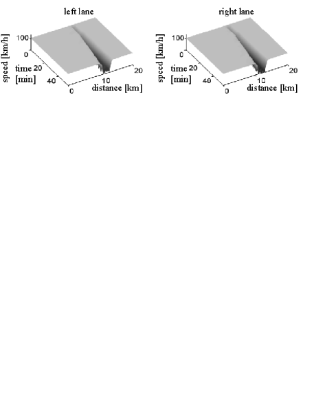
Figure 6: Simulation of traffic congestion under breakdown vehicle ahead without communication.

Now we consider the same scenario for the case of communicating vehicles, which sent $``$dange warning” message about the breakdown vehicle ahead. We assume that after the communicating vehicles have received this message they increase the distance to 600 m at which the communicating vehicles moving in the right lane try to change to the left lane. Because we assume that vehicles, which cannot communicate, begin to change the lane at the distance 100 m, the simulation results depend on the percentage of the communicating vehicles as presented in Fig. 7 .

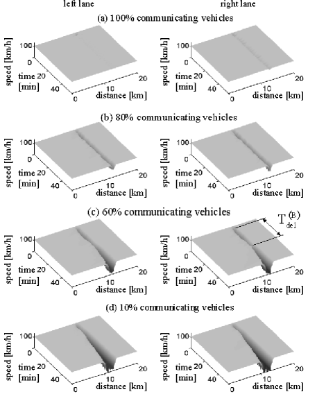
Figure 7: Simulation of effect on traffic congestion of danger warning for different pecentage of communicating vehicles

We can see that there is a critical percentage of the communicating vehicles that is about 70$\%$ (Fig. 7): (i) if the percentage of the communicating vehicles is greater than the critical one, then no traffic congestion occurs. (ii) Otherwise, a congested pattern occurs whose downstream front is fixed at the location of the breakdown vehicle; characteristics of this congested patterns are similar to those as for the case when no communication vehicles moving in traffic flow (Fig. 6). However, we should note that when the percentage of the communicating vehicles is smaller but close to the critical value, then there is a random time delay in the occurrence of the congested pattern that is denoted by $T_{\rm del}^{\rm(B)}$ in Fig. 6 (c). The time delay is a random value: at the same simulation parameters but different initial spatial distributions of traffic variables very different values $T_{\rm del}^{\rm(B)}$ are found.

5 Prevention of Traffic Breakdown at On-Ramp Bottleneck Through Vehicle Ad-Hoc Network

In accordance with three-phase traffic theory [22, 23], we can assume that there can be the following two hypothetical possibilities to prevent traffic breakdown at an on-ramp bottleneck through changes in driver behavior of communicating vehicles:

(i) A decrease in the amplitude of disturbances on the main road occurring when vehicles merge from on-ramp onto the right lane of the main road. This decreases the probability of nucleus occurrence required for traffic breakdown.

(ii) An increase in probability of over-acceleration.

Figure 8: Simulations of prevention of traffic breakdown at on-ramp bottleneck through vehicle communication: Speed in time and space without communication (a) and with vehicle communication (b).

In simulations (Fig. 8), there is an on-ramp bottleneck at location 16 km. The flow rate on the main road upstream of the bottleneck is $q_{\rm in}=$ 1827 vehicles/h/lane; the flow rate to the on-ramp is $q_{\rm on}=$ 600 vehicles/h. At these flow rates if there is no C2C communication, a general congested pattern (GP) [22] occurs at the bottleneck (Fig. 8 (a)). The GP consists of a pinch region of synchronized flow (labeled by $``$pinch region”) and wide moving jams upstream of the pinch region (labeled by $``$wide moving jams”).

Now we assume (Fig. 8 (b)) that all vehicles are communicated vehicles, which try to send a non-priority message with time intervals 0.1 s. Vehicles moving in the on-ramp lane send a priority message for neighbor vehicles moving in the right road lane when the vehicle intends to merge from the on-ramp onto the main road. We assume that the following vehicle in the right lane increases a time headway for the vehicle merging. Simulations show that in comparison with the case in which no vehicle communication is applied and the GP occurs (Fig. 8 (a)) this change in driver behavior of communicating vehicles decreases disturbances in free flow at the bottleneck. This results in the prevention of traffic breakdown (Fig. 8 (b)).

6 Effect of Ad-Hoc Vehicle Network on Congested Traffic Patterns

Here we consider a case of the same communicating vehicles as that in Sect. 5 at $q_{\rm in}=$ 1946 vehicles/h/lane when traffic control through the use of changes in driver behavior in free flow at the bottleneck discussed above is not applied. In this case, traffic breakdown occurs at the bottleneck resulting in GP occurrence (Fig. 9 (a, b)). In accordance with three-phase traffic theory [22, 23], we can assume that there can be the following two hypothetical possibilities to prevent moving jam emergence in synchronized flow through changes in driver behavior of communicating vehicles moving in synchronized flow:

(i) A decrease in the amplitude of disturbances in synchronized flow upstream of the bottleneck. This decreases the probability of nucleus occurrence required for the emergence of wide moving jams.

(ii) A decrease in the density of synchronized flow upstream of the bottleneck. This decreases the critical speed required for the emergence of wide moving jams in synchronized flow. The lower the critical speed, the smaller the probability for the emergence of wide moving jams.

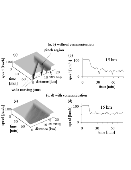
Figure 9: Simulation of the effect of vehicle communication on congested patterns: Speed in time and space (a, c) and at a location $x=$ 15 km (b, d) without communication (a, b) and with communication (c, d).

We assume that after synchronized flow has just occurred due to traffic breakdown at the bottleneck, communicating vehicles, which reach the synchronized flow, send priority messages about the speed reduction to vehicles moving in free flow upstream. Each message comprises a minimum space gap that should be maintained by vehicles while moving in the synchronized flow.

In vehicle motion rules of the model, the associated change in driver behavior is simulated through an increase in probability $p_{1}$ in (17) from 0.3 for vehicles, which have no information about the required space gap to 0.55 for the vehicles that received the message. The greater $p_{1}$, the greater the difference between vehicle space gap and a safe space gap and, therefore, the less the probability for moving jam emergence in the synchronized flow [22]. As a result of space gap increase within the synchronized flow, at the same flow rates upstream of the bottleneck as those in Fig. 9 (a, b) rather than the GP a widening synchronized flow pattern (WSP) is forming (Fig. 9 (c, d)). Whereas in the pinch region of the GP the mean space gap is 15 m, it is 25 m within the WSP. Due to the transformation of the GP into the WSP, two effects are achieved: (i) wide moving jams do not occur and (ii) the average speed within synchronized flow upstream of the bottleneck increases from about 40 km/h within the GP to 60 km/h within the WSP. These effects can result in a considerable increase in the efficiency and safety of traffic.

7 Conclusion

1. Simulations made with the use of the testbed for ad-hoc networks presented in this paper allow us to perform quick simulations of various applications of C2C-communication and ad-hoc network performance associated with the real behavior of vehicular traffic. This is due of the following advantages of this testbed: As in a real ad-hoc network, there is only one network in the testbed in which C2C-communication, ad-hoc performance, and traffic flow characteristics are simulated simultaneously during vehicle motion. This testbed feature decreases the simulation run time considerably and exhibits a sufficient accuracy of simulations. This testbed feature allows us to make an easier understanding of ad-hoc network and traffic flow performances associated with those applications in which message contexts should influence on vehicle behavior. This is crucial especially for communication based safety systems that currently are studied in various research projects (e.g. WILLWARN [5] and SAFESPOT [26]).

2. Simulations show that changes in driver behavior made through the use of ad-hoc vehicle network can indeed prevent traffic breakdown and/or lead to the dissolution of moving jams. Thus C2X communication can increase the efficiency and safety of traffic considerably.

Appendix A Stochastic Three-Phase Traffic Flow Model

Basic rules of vehicle motion in the model are as follows [24, 25]:

$$v_{n+1}=\max(0,\min({v_{\rm free},\tilde{v}_{n+1}+\xi_{n},v_{n}+a\tau,v_{{\rm s},n}})),$$ (2)

$$x_{n+1}=x_{n}+v_{n+1}\tau,$$ (3)

$$\tilde{v}_{n+1}=\max(0,\min({v_{\rm free},v_{{\rm c},n},v_{{\rm safe},n}})),$$ (4)

(5)

$$v_{c,n}=\left\{\begin{array}[]{ll}v_{n}+\Delta_{n}&\textrm{at $g_{n}\leq G_{n}$}\\ v_{n}+a_{n}\tau&\textrm{at $g_{n}>G_{n}$},\end{array}\right.$$ (8)

where

$$\Delta_{n}=\max(-b_{n}\tau,\min(a_{n}\tau,\ v_{\ell,n}-v_{n})),$$ (9)

$v_{\rm free}$ is the maximum speed in free flow that is constant, $g_{n}=x_{\ell,n}-x_{n}-d$ is the space gap, $x_{n}$ is the vehicle co-ordinate, the lower index $\ell$ marks functions and values related to the preceding vehicle; all vehicles have the same length $d$; index $n$ corresponds to the discrete time $t=n\tau$, $n=0,1,2,...;$ $\tau$ is time step; a synchronization space gap $G_{n}$ and a safe speed $v_{\rm safe,n}$ have been discussed in [22] in detail. Steady states of this model, i.e., states in which all vehicles move at a time-independent speed at the same space gap between each other cover a 2D-region in the flow–density plane (Fig. 10).

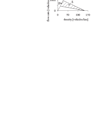
Figure 10: Steady speed states for the Kerner-Klenov stochastic three-phase traffic flow in the flow–density plane

Random deceleration and acceleration $\xi_{n}$ in (2) are applied depending on whether the vehicle decelerates or accelerates, or else maintains its speed:

$$\xi_{n}=\left\{\begin{array}[]{ll}-\xi_{\rm b}&\textrm{if $S_{n+1}=-1$}\\ \xi_{\rm a}&\textrm{if $S_{n+1}=1$}\\ 0&\textrm{if $S_{n+1}=0$},\end{array}\right.$$ (10)

where $S$ in (10) denotes the state of motion ($S_{n+1}=-1$ represents deceleration, $S_{n+1}=1$ acceleration, and $S_{n+1}=0$ motion at nearly constant speed)

$$S_{n+1}=\left\{\begin{array}[]{ll}-1&\textrm{if $\tilde{v}_{n+1}<v_{n}-\delta$}\\ 1&\textrm{if $\tilde{v}_{n+1}>v_{n}+\delta$}\\ 0&\textrm{otherwise},\end{array}\right.$$ (11)

where $\delta$ is constant ($\delta\ll a\tau$).

$$\xi_{\rm a}=a\tau\Theta(p_{\rm a}-r),$$ (12)

where $p_{\rm a}$ is probability of random acceleration, $a$ is the maximum acceleration, $r={\rm rand(0,1)}$, $\Theta(z)=0$ at $z<0$ and $\Theta(z)=1$ at $z\geq 0$;

$$\xi_{\rm b}=a\tau\Theta(p_{\rm b}-r),$$ (13)

Random acceleration $a_{n}$ and deceleration $b_{n}$ are

$$a_{n}=a\Theta(P_{\rm 0}-r_{1}),$$ (14)

$$b_{n}=a\Theta(P_{\rm 1}-r_{1}),$$ (15)

where the probabilities $P_{0}$ and $P_{1}$ are

$$P_{0}=\left\{\begin{array}[]{ll}p_{0}(v_{n})&\textrm{if $S_{n}\neq 1$}\\ 1&\textrm{if $S_{n}=1$},\end{array}\right.$$ (16)

$$P_{1}=\left\{\begin{array}[]{ll}p_{1}&\textrm{if $S_{n}\neq-1$}\\ p_{2}(v_{n})&\textrm{if $S_{n}=-1$},\end{array}\right.$$ (17)

$r_{1}={\rm rand(0,1)}$, speed functions for probabilities $p_{0}(v_{n})$ and $p_{2}(v_{n})$ are considered in [22]; $p_{1}$ is constant. Lane changing rules, models of highway bottlenecks and other model parameters in all simulations presented in the article are listed in Table 16.11 of the book [22].

References

- [1] Dedicated Short Range Communications working group. http://grouper.ieee.org/groups/scc32/dsrc/index.html
- [2] The Fleetnet Project. http://www.fleetnet.de
- [3] The Now: Network on Wheels Project. http://www.network-on-wheels.de
- [4] Internet ITS Consortium. http://www.internetits.org
- [5] The WILLWARN Project. http://www.prevent-ip.org/en/
- [6] Vehicle safety communications consortium. http://www- nrd.nhtsa.dot.gov/pdf/nrd-12/CAMP3/pages/VSCC.htm
- [7] Car2Car Communication Consortium. http://www.car-to-car.org/
- [8] Network Simulator ns-2. http://www.isi.edu/nsnam/ns
- [9] R. Schmitz, M. Torrent-Moreno, H. Hartenstein, W. Effelsberg, in Proceeding of 29th Annual IEEE International Conference on Local Computer Networks, (IEEE, Tampa, Florida, 2004), pp. 594–601
- [10] M. Torrent-Moreno, D. Jiang, H. Hartenstein, in VANET’04: Proceedings of the 1st ACM International Workshop on Vehicular Ad Hoc Networks, (Philadelphia, Pennsylvania, 2004), pp. 10–18
- [11] M. Torrent-Moreno, S. Corroy, F. Schmidt-Eisenlohr, H. Hartenstein, in MSWiM’06: Proceedings of the 9th ACM international Symposium on Modeling Analysis and Simulation of Wireless and Mobile Systems, (Terromolinos, Spain, 2007), pp. 68–77
- [12] F. Schmidt-Eisenlohr, M. Torrent-Moreno, J. Mittag, H. Hartenstein, in WONS’07: Proceedings of the Fourth Annual Conference on Wireless on Demand Network Systems and Services, (Obergurgl, Austria, 2007), pp. 50–58
- [13] D. Choffnes, F. Bustamante, in Proceedings of the International Workshop on Vehicular Ad Hoc Networks, (Cologne, Germany, 2005)
- [14] J. Maurer, T. F gen, W. Wiesbeck, in Proceedings of the International Workshop on Intelligent Transportation, (Hamburg, Germany, March 2005).
- [15] Q. Chen, D. Jiang, V. Taliwal, L. Delgrossi, in Proceedings of the International Workshop on Vehicular Ad Hoc Networks, (Los Angeles, 2006)
- [16] First Simulation Workshop 2007. http://www.comesafety.org/index.php?id=34
- [17] B. Sklar, IEEE Communications Magazine, 35, 90–100 (1997)
- [18] B. S. Kerner, S. L. Klenov, A. Brakemeier, arXiv: 0712.2711 (2007), available at http://arxiv.org/abs/0712.2711; in Proceedings of IEEE IV 2008, paper 35; in Proceedings of the Fourth international Workshop on Vehicle-to-Vehicle Communication V2VCOM 2008, (2008), pp. 57–63
- [19] IEEE Std.802.11-1999, Part 11: Wireless LAN Medium Access Control (MAC) and Physical Layer (PHY) specifications. IEEE Std.802.11, 1999 edition.
- [20] IEEE Std.802.11e/D4.4, Draft Supplement to Part 11: Wireless LAN Medium Access Control (MAC) and Physical Layer (PHY) specifications: Higher-speed Physical Layer the 5 GHz Band, IEEE Std.802.11a-1999, 1999.
- [21] IEEE Std.802.11a, Supplement to Part 11: Wireless LAN Medium Access Control (MAC) and Physical Layer (PHY) specifications: Medium Access Control (MAC) Enhancements for Quality of Service (QoS), June 2004.
- [22] B.S. Kerner, The Physics of Traffic, (Springer, Berlin, New York, 2004)
- [23] B.S. Kerner, Introduction to Modern Traffic Flow Theory and Control: The Long Road to Three-Phase Traffic Theory, (Springer, Berlin, New York, 2009)
- [24] B.S. Kerner, S.L. Klenov. A microscopic model for phase transition in traffic flow. J. Phys. A: Math. Gen., 35, L31-L43 (2002).
- [25] B.S. Kerner, S.L. Klenov. A microscopic theory of spatial-temporal congested traffic patterns at highway bottlenecks. Phys. Rev. E, 68, 036130 (2003).
- [26] SAFESPOT, Integrated Project, http://www.safespot-eu.org/pages/page.php